matlab绘制简易二维图
实验二MATLAB绘制图形
grid on %在所画出的图形坐标中加入栅格
绘制图形如下
50
10
1
0.8
40
10
0.6
0.4
30
10
0.2
0
1020
-0.2
-0.4
1010
-0.6
-0.8
0
10
-1
-2
0
2
-2
0
2
10
10
10
10
10
10
如果在图中不加栅格
程序如下:
clear x=logspace(-1,2);%在10^(-1)到10^2之间产生50个 对数等分的行向量 subplot(121); loglog(x,10*exp(x),'-p') subplot(122); semilogx(x,cos(10.^x))
(2)plot(x,y): 基本格式,x和y可为向量或矩阵. 1. 如果x,y是同维向量,以x元素为横坐标,以y元素 为纵坐标绘图. 2. 如果x是向量,y是有一维与x元素数量相等的矩阵, 则以x为共同横坐标, y元素为纵坐标绘图,曲线数目 为y的另一维数. 3. 如果x,y是同维矩阵,则按列以x,y对应列元素为 横、纵坐标绘图,曲线数目等于矩阵列数.
y=2*exp(-0.5*x).*cos(4*pi*x);
2
plot(x,y)
1.5
1
0.5
0
-0.5
-1
-1.5
-2
0
1
2
3
4
5
6
7
例4 绘制曲线
t=(0:0.1:2*pi);
x=t.*sin(3*t);
y=t.*sin(t).*sin(t);
MATLAB4二维图形绘制
y3=cos(t);y4=cos(t+0.25);y5=cos(t+0.5); plot(t,y3);hold on; plot(t,y4); plot(t,y5);
1 0.8 0.6 0.4 0.2 0 -0.2 -0.4 -0.6 -0.8 -1 0 1 2 3 4 5 6 7
0
figure(1) title('\fontsize{16}y(\omega)=\int^{\infty }_{0}y(t)e^{-j\omegat}dt')
二、绘制曲线的一般步骤
步骤 1 表 4.1 绘制二维、三维图形的一般步骤 内容 曲线数据准备: 对于二维曲线,横坐标和纵坐标数据变量; 对于三维曲面,矩阵参变量和对应的函数值。 指定图形窗口和子图位置: 默认时,打开 Figure No.1 窗口或当前窗口、当前子图; 也可以打开指定的图形窗口和子图。 设置曲线的绘制方式: 线型、色彩、数据点形。 设置坐标轴: 坐标的范围、刻度和坐标分格线 图形注释: 图名、坐标名、图例、文字说明 着色、明暗、灯光、材质处理(仅对三维图形使用) 视点、三度(横、纵、高)比(仅对三维图形使用) 图形的精细修饰(图形句柄操作): 利用对象属性值设置; 利用图形窗工具条进行设置。
x=peaks;plot(x) x=1:length(peaks);y=peaks;plot(x,y)
10 8 6 4 2 0 -2 -4 -6 -8
0
5
10
15
20
25
30
35
40
45
50
3. 单窗口多曲线分图绘图 subplot(1,3,1); plot(t,y) subplot(1,3,2); plot(t,y3) subplot(1,3,3); plot(t,y2)
数学2-用MATLAB绘制二维-三维图形(lq)

[i,j,v]=find(A) 返回矩阵A中非零元素所在的行i,
列j,和元素的值v(按所在位置先后 顺序输出)
A=[3 2 0; -5 0 7; 0 0 1]; [i,j,v]=find(A)
i= 1 2 1 2 3 j= 1 1 2 3 3 v = 3 -5 2 7 1
[X,Y]=meshgrid(x,y) 3)根据函数表达式生成全部网格节点出对应的函数值矩阵z: z=f(X,Y) 4)顺序连接已经产生的空间点(x,y,z)绘制相应曲面: mesh(X,Y,Z) surf(X,Y,Z) shading flat %去除网格线。
例2-7画出矩形域[-1,1]×[-1,1]旋转抛物面:z=x2+y2. x=linspace(-1,1,100); y=x; [X,Y]=meshgrid(x,y); %生成矩形区[-1,1]×[-1,1]的网格坐标矩阵 Z=X.^2+Y.^2; subplot(1,2,1) mesh(X,Y,Z); subplot(1,2,2) surf(X,Y,Z); shading flat; %对曲面z=x2现方式做保护处理对用户上传分享的文档内容本身不做任何修改或编辑并不能对任何下载内容负责
用matlab绘制二维、三维图形
2.1二维图形的绘制
2.1.1 二维绘图的基本命令 matlab中,最常用的二维绘图命令是plot。
使用该命令,软件将开辟一个图形窗口,并 画出连接坐标面上一系列点的连线。
例2-5 采用不同形式(直角坐标、参数、极坐标),画出 单位圆x2+y2=1的图形。
分析:对于直角坐标系方程,y= 1 x2,对于参数方 程x=cost,y=sint,t[0,2 pi] ,利用plot(x,y)命令可以实现。 而在极坐标系中单位圆为r=1(1+0t),利用polar(t,r)命 令实现。
实验五 MATLAB二维、三维图形的绘制

实验五 MATLAB二维、三维图形的绘制一、实验目的1.掌握二维、三维图形的绘制;2.掌握特殊二维图形的绘制;3.掌握绘图参数的设置;4.了解并学习简单动画的制作。
二、实验内容1.运行下列程序,学会并掌握标题、坐标轴标签和网格线的设置方法x=0:1:10;y=x.^2-10*x+6;plot(x,y);title ('Plot of y=x.^2-10*x+6');xlabel ('x');ylabel ('y');grid on;2.运行下列程序,学会并掌握线型、点型、颜色的设置方法x = -pi:pi/20:pi;y1 = sin(x);y2 = cos(x);plot(x,y1,'bo',x,y2,'r:');title('线型、点型和颜色');xlabel('时间'),ylabel('Y');grid on;3.同一坐标系内多条曲线的绘制1)使用 plot(x,[y1;y2;…])x = -pi:pi/20:pi;y1 = sin(x);y2 = cos(x);plot(x,[y1;y2]);legend('sin x','cos x');2)使用hold命令x = -pi:pi/20:pi;y1 = sin(x);y2 = cos(x);plot(x,y1);hold on;plot(x,y2,‘r’);3)在plot后使用多输入变量x = -2*pi:pi/20:2*pi;y1 = 2*sin(x);y2 = 2*cos(x);plot(x,y1,'ro',x,y2,'b:');title('线型、点型和颜色');xlabel('时间'),ylabel('Y');4) 使用plotyy命令x = -pi:pi/20:pi;y1 = sin(x);y2 = 5*cos(x);plotyy(x,y1,x,y2);grid on;gtext(‘sinx’) ; gtext(‘5cosx’) ;4.子图形窗口的绘制subplot(2,1,1);x= -pi:pi/20:pi;y=sin(x);plot(x,y) ; grid on;title('正弦曲线');subplot(2,1,2);x= -pi:pi/20:pi;y=cos(x);plot(x,y); grid on;title('余弦曲线');5.对数坐标图形x=0:0.1:10;y=x.^2 -10.*x +25;subplot(2,2,1);plot(x,y); grid on;xlabel('a) x、y轴线性刻度');subplot(2,2,2);semilogx(x,y); grid on;xlabel('b) x轴对数刻度、y轴线性刻度');subplot(2,2,3);semilogy(x,y); grid on;xlabel('c) x轴线性刻度、y轴对数刻度');subplot(2,2,4);loglog(x,y); grid on;xlabel(‘d) x、y轴对数刻度');6.极坐标下的绘图theta = 0:pi/20:2*pi;r = 0.5+cos(theta);polar(theta,r);7.复数的绘图,并比较下面几种情况的不同1)t = 0:pi/20:6*pi;y = exp(0.1*t) .* (cos(t) + i * sin(t));plot(y);grid on ;title('Plot of Complex Function vs Time');xlabel('Real Part');ylabel('Imaginary Part');2)t = 0:pi/20:6*pi;y = exp(0.1*t) .* (cos(t) + i * sin(t));plot(t, y);grid on ;title('Plot of Complex Function vs Time');xlabel('t');ylabel('y(t)');3)t = 0:pi/20:6*pi;y = exp(0.1*t) .* (cos(t) + i * sin(t));plot(t, real(y),'b-');grid on;hold on;plot(t, imag(y),'r-');title('Plot of Complex Function vs Time');xlabel('t');ylabel('y(t)');legend('real','imaginary');hold off;4)t = 0:pi/20:6*pi;y = exp(0.1*t) .* (cos(t) + i * sin(t));polar(angle(y),abs(y));title('Plot of Complex Function');8.特殊二维图形的绘制1)x = [1 2 3 4 5 6];y = [2 6 8 7 8 5];stem(x,y);title('Example of a Stem Plot');xlabel('x');ylabel('y');axis([0 7 0 10]);将上述程序中的stem语句换为stairs、bar、barh和compass,即可实现阶梯图、条形图、罗盘图的绘制。
第5章matlab绘制二维图形及三维图形的方法
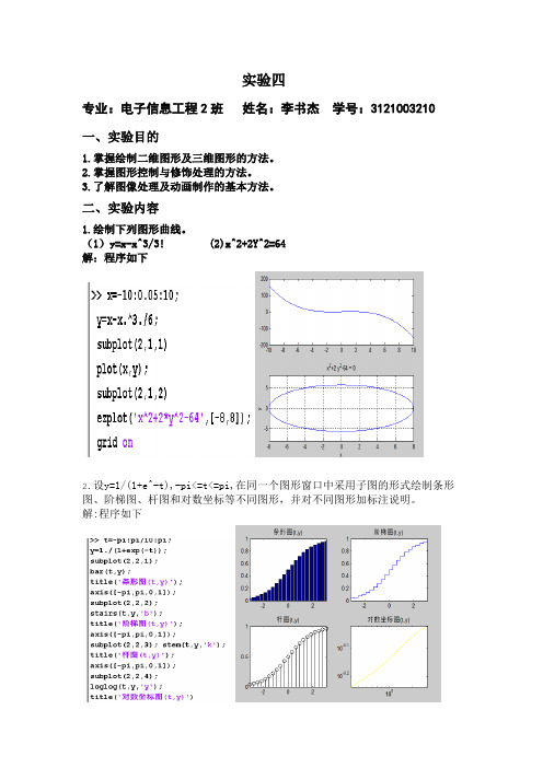
实验四
专业:电子信息工程2班姓名:李书杰学号:3121003210
一、实验目的
1.掌握绘制二维图形及三维图形的方法。
2.掌握图形控制与修饰处理的方法。
3.了解图像处理及动画制作的基本方法。
二、实验内容
1.绘制下列图形曲线。
(1)y=x-x^3/3! (2)x^2+2Y^2=64
解:程序如下
2.设y=1/(1+e^-t),-pi<=t<=pi,在同一个图形窗口中采用子图的形式绘制条形图、阶梯图、杆图和对数坐标等不同图形,并对不同图形加标注说明。
解:程序如下
3.绘制下列极坐标图。
(1)ρ=5cosθ+4 (2)γ=5sin^2φ/cosφ,-π/3<φ<π/3 解:程序如下
思考练习:
2.绘制下列曲线
(1)y=1/2πe^(-x^2/2) (2)x=tsint y=tcost
解:程序如下
(1)
结果如下:
(2)
结果如下:
3.在同一坐标中绘制下列两条曲线并标注两曲线交叉点。
(1)y=2x-0.5
(2)x=sin(3t)cost
Y=sin(3t)sint
解:程序如下
4.分别用plot和fplot函数绘制y=sin(1/x)的曲线,分析两曲线的差别。
解:程序如下
结果如下:
5.绘制下列极坐标图:
(1)p=12/sqrt(θ) (2)γ=3asinφcosφ/(sin^3φ+cos^3φ)解:程序如下
结果如下:。
matlab实验三二维图形和三维图形的创建
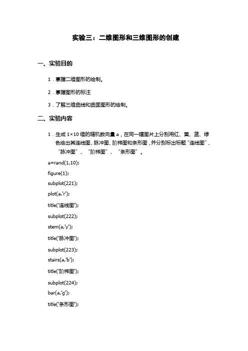
实验三:二维图形和三维图形的创建一、实验目的1.掌握二维图形的绘制。
2.掌握图形的标注3.了解三维曲线和曲面图形的绘制。
二、实验内容1.生成1×10维的随机数向量a,在同一幅图片上分别用红、黄、蓝、绿色绘出其连线图、脉冲图、阶梯图和条形图,并分别标出标题“连线图”、“脉冲图”、“阶梯图”、“条形图”。
a=rand(1,10);figure(1);subplot(221);plot(a,'r');title('连线图');subplot(222);stem(a,'y');title('脉冲图');subplot(223);stairs(a,'b');title('阶梯图');subplot(224);bar(a,'g');title('条形图');2.绘制向量x=[1 3 0.5 2.5 2]的饼形图,并把3对应的部分分离出来。
x=[1 3 0.5 2.5 2];pie(x,[0 3 0 0 0]);3.用hold on命令在同一个窗口绘制曲线y=sin(t),y1=sin(t+0.25)y2=sin(t+0.5),其中t=[0 10]。
t=0:pi/100:10y=sin(t);y1=sin(t+0.25);y2=sin(t+0.5);plot(t,y);hold on;plot(t,y1);hold on;plot(t,y2);hold on;4.绘制曲线 x=tcos(3t)y=tsin2t 其中-π≤t≤π,步长取π/100。
要求:要图形注解、标题、坐标轴标签, 并在曲线上截取一点,将相对应的坐标值文本标注出来(ginput())。
;t=-pi:pi/100:pi;x=t.*cos(3*t);y=t.*(sin(t.^2));plot(t,x,'g-',t,y,'r-');title('曲线');xlabel(t,'Fontsize',12);ylabel('幅值','Fontsize',12);[x y]=ginput(1)5.在三个子图像中,分别绘制三维曲线,三维曲面,三维网格的半径为6,坐标为(6,7,6)的由900个面构成的球面(sphere()),对每个图形标注标题6.(1)绘一个圆柱螺旋线(形似弹簧)图。
matlab二维图形的绘制
matlab二维图形的绘制(2006-11-20 20:38:35)转载▼分类:matlab基础(电子方向)常用的二维图形命令:plot:绘制二维图形loglog:用全对数坐标绘图semilogx:用半对数坐标(X)绘图semilogy:用半对数坐标(Y)绘图fill:绘制二维多边填充图形polar:绘极坐标图bar:画条形图stem:画离散序列数据图stairs:画阶梯图errorbar:画误差条形图hist:画直方图fplot:画函数图title:为图形加标题xlabel:在X轴下做文本标记ylabel:在Y轴下做文本标记zlabel:在Z轴下做文本标记text:文本注释grid:对二维三维图形加格栅绘制单根二维曲线plot函数,基本调用格式为:plot(x,y)其中x和y为长度相同的向量,分别用于存储x坐标和y坐标数据。
例如:在区间内,绘制曲线y=2e-0.5xcos(4πx)程序如下:x=0:pi/100:2*pi;y=2*exp(-0.5*x).*cos(4*pi*x);plot(x,y)plot函数最简单的调用格式是只包含一个输入参数:plot(x)在这种情况下,当x是实向量时,以该向量元素的下标为横坐标,元素值为纵坐标画出一条连续曲线,这实际上是绘制折线图。
p=[22,60,88,95,56,23,9,10,14,81,56,23];plot(p)绘制多根二维曲线1.plot函数的输入参数是矩阵形式(1) 当x是向量,y是有一维与x同维的矩阵时,则绘制出多根不同颜色的曲线。
曲线条数等于y矩阵的另一维数,x被作为这些曲线共同的横坐标。
(2) 当x,y是同维矩阵时,则以x,y对应列元素为横、纵坐标分别绘制曲线,曲线条数等于矩阵的列数。
(3) 对只包含一个输入参数的plot函数,当输入参数是实矩阵时,则按列绘制每列元素值相对其下标的曲线,曲线条数等于输入参数矩阵的列数。
当输入参数是复数矩阵时,则按列分别以元素实部和虚部为横、纵坐标绘制多条曲线。
二维图形的绘制

依次输入如下指令,观察输出的图形.
>> x=[0:0.2:2*pi];
红色、虚线、 离散点用加号
>> plot(x,cos(x));
>> plot(x,cos(x),’r+:’); 属性可以全部指定,也
>> plot(x,cos(x),’bd-.’); 可以只指定其中某几个 >> plot(x,cos(x),’k*-’); 排列顺序任意
x=0:0.01:4*pi; y1=exp(-0.5*x); y2=-exp(-0.5*x); y3=exp(-0.5*x).*sin(5*x); plot(x,y1,x,y2,x,y3)
函数线条会自动设 置成不同颜色
数组间的乘法用.*
习题 使用plot函数绘制
y 10*exp((0.2 pi)* x), x 0,10
例2 使用plot(x,y)命令绘制y=cosx在[-4π,4π]的图形.
Matlab作图步骤:
给出离散点列: x=-4*pi:0.1:4*pi 计算函数值: y=cos(x) 画图:用 matlab 二维绘图命令 plot 作出函数图形
plot(x,y)
作图命令:x=-4*pi:0.1:4*pi; y=cos(x); plot(x,y)
>> x=0:0.01:10; >> y=10*exp((-0.2+pi)*x); >> plot(x,y)
Matlab 作图
2、Matlab作图命令: (2)plot(x,y,'LineSpec')
- 1、下载文档前请自行甄别文档内容的完整性,平台不提供额外的编辑、内容补充、找答案等附加服务。
- 2、"仅部分预览"的文档,不可在线预览部分如存在完整性等问题,可反馈申请退款(可完整预览的文档不适用该条件!)。
- 3、如文档侵犯您的权益,请联系客服反馈,我们会尽快为您处理(人工客服工作时间:9:00-18:30)。
图1图2图3三幅图的matlab绘图指令图1的matlab绘图指令C=[0,0];B=[600/2,-600*sqrt(3)/2];plot([C(1),B(1)],[C(2),B(2)],'k-'),hold onaxis equalD=[B(1)-B(2),0];plot([D(1),B(1)],[D(2),B(2)],'k-'),hold onplot([C(1)-50,D(1)+50],[C(2),D(2)],'k-','LineWidth',2),hold onn=20;yinying=zeros(2,n+1);yinying(1,1:n+1)=(C(1)-50):((D(1)+50)-(C(1)-50))/n:(D(1)+50);yinying(2,1:n+1)=zeros(1,n+1);yinying(3,1:n+1)=yinying(1,1:n+1)+20*ones(1,n+1);yinying(4,1:n+1)=yinying(2,1:n+1)+20*ones(1,n+1);for ii=1:n+1plot([yinying(1,ii),yinying(3,ii)],[yinying(2,ii),yinying(4,ii)],'k-'),hold on endplot(C(1),C(2),'k-', 'Marker','.','MarkerSize',15)plot(B(1),B(2),'k.', 'Marker','.','MarkerSize',15)plot(D(1),D(2),'k.', 'Marker','.','MarkerSize',15)text(C(1)-30,C(2)-20,'C');text(B(1)+20,B(2),'B');text(D(1)+10,D(2)-20,'D');text(B(1)+20,B(2)-200,'P','FontWeight','Bold');text(C(1)-100,C(2)-100,'L_{BC}=600mm');text(B(1)-100,B(2)+200,'\alpha=30^{。
}');text(B(1)+50,B(2)+180,'\beta=45^{。
}');plot([B(1),B(1)],[B(2),B(2)+200],'k-.'),hold onplot([B(1),B(1)],[B(2),B(2)-200],'k-','LineWidth',1.5),hold onarrow_P=[B(1),B(1)+8,B(1)-11;B(2)-200,B(2)-200+30,B(2)-200+30];fill(arrow_P(1,:),arrow_P(2,:),'k')axis([-200,1000,-800,100])theta=90:(120-90)/30:120;theta=theta*pi/180;r=100;x0=B(1);y0=B(2);x=x0+r*cos(theta);y=y0+r*sin(theta);plot(x,y,'k-'),hold ontheta=45:(120-90)/45:90;theta=theta*pi/180;r=150;x0=B(1);y0=B(2);x=x0+r*cos(theta);y=y0+r*sin(theta);plot(x,y,'k-'),hold onbox off图2的matlab绘图指令为% cantilever_beam 绘图clear allA=[0,-10];B=[0,10];C=[50,-10];D=[50,10];plot([A(1),C(1)],[A(2),C(2)],'k-','LineWidth',1.5),hold onplot([B(1),D(1)],[B(2),D(2)],'k-','LineWidth',1.5),hold onplot([D(1),C(1)],[D(2),C(2)],'k-','LineWidth',1.5),hold onplot([A(1),B(1)],[A(2)-10,B(2)+10],'k-','LineWidth',1.5),hold on axis equalE=[0,0];F=[100,0];plot([E(1),F(1)],[E(2),F(2)],'k-.'),hold onG=[50,-5];H=[50,5];K=[100,-5];L=[100,5];plot([G(1),K(1)],[G(2),K(2)],'k-','LineWidth',1.5),hold onplot([H(1),L(1)],[H(2),L(2)],'k-','LineWidth',1.5),hold onplot([K(1),L(1)],[K(2),L(2)],'k-','LineWidth',1.5),hold onplot([C(1),C(1)],[C(2),C(2)-10],'k-','LineWidth',1),hold onplot([K(1),K(1)],[K(2),K(2)-15],'k-','LineWidth',1),hold onplot([0,22],[-15,-15],'k-','LineWidth',1),hold onplot([28,72],[-15,-15],'k-','LineWidth',1),hold onplot([78,100],[-15,-15],'k-','LineWidth',1),hold onarrow_P=[0+4,0,0+4;-15-1,-15,-15+1];fill(arrow_P(1,:),arrow_P(2,:),'k')arrow_P=[50-4,50,50-4;-15-1,-15,-15+1];fill(arrow_P(1,:),arrow_P(2,:),'k')arrow_P=[50+4,50,50+4;-15-1,-15,-15+1];fill(arrow_P(1,:),arrow_P(2,:),'k')arrow_P=[100-4,100,100-4;-15-1,-15,-15+1];fill(arrow_P(1,:),arrow_P(2,:),'k')plot([F(1),F(1)+15],[F(2),F(2)],'k-','LineWidth',1),hold onarrow_P=[F(1)+11,F(1)+15,F(1)+11;F(2)-1,F(2),F(2)+1];fill(arrow_P(1,:),arrow_P(2,:),'k')n=30;yinying=zeros(4,n+1);yinying(1,1:n+1)=zeros(1,n+1);yinying(2,1:n+1)=(A(2)-10):(((B(2)+10))-(A(2)-10))/n:(B(2)+10);yinying(3,1:n+1)=yinying(1,1:n+1)-3*ones(1,n+1);yinying(4,1:n+1)=yinying(2,1:n+1)+3*ones(1,n+1);for ii=1:n+1plot([yinying(1,ii),yinying(3,ii)],[yinying(2,ii),yinying(4,ii)],'k-'),hold on endplot(E(1),E(2),'k-', 'Marker','.','MarkerSize',15)plot(F(1),F(2),'k.', 'Marker','.','MarkerSize',15)plot(50,0,'k.', 'Marker','.','MarkerSize',15)text(25,13,'I_{1}','fontname','华文仿宋','FontAngle','italic');text(75,8,'I_{2}','fontname','华文仿宋','FontAngle','italic');text(101,18,'P','FontWeight','Bold');text(116,0,'x');text(0,33,'y');text(E(1)+1,E(2)-2.5,'1');text(50+1,0-2.5,'2');text(F(1)+1,F(2)-2.5,'3');z=text(24,-15,'$$\frac{L}{2}$$');set(z,'Interpreter','latex');z=text(74,-15,'$$\frac{L}{2}$$');set(z,'Interpreter','latex');plot([B(1),B(1)],[B(2)+10,B(2)+20],'k-','LineWidth',1),hold onarrow_P=[B(1)-1,B(1),B(1)+1;B(2)+16,B(2)+20,B(2)+16];fill(arrow_P(1,:),arrow_P(2,:),'k')plot([L(1),L(1)],[L(2),L(2)+20],'k-','LineWidth',1.5),hold onarrow_P=[L(1)-1,L(1),L(1)+1;L(2)+4,L(2),L(2)+4];fill(arrow_P(1,:),arrow_P(2,:),'k')plot([F(1),F(1)+15],[F(2),F(2)],'k-','LineWidth',1),hold onarrow_P=[F(1)+11,F(1)+15,F(1)+11;F(2)-1,F(2),F(2)+1];fill(arrow_P(1,:),arrow_P(2,:),'k')axis([-10,130,-35,40])box off图3的matlab绘图指令为% thin_slab 绘图P1=[0,0];P2=[0,40];P3=[50,20];P4=[100,0];P5=[100,40];plot([P1(1),P2(1)],[P1(2),P2(2)],'k-','LineWidth',1.5),hold onplot([P1(1),P4(1)],[P1(2),P4(2)],'k-','LineWidth',1.5),hold onplot([P5(1),P4(1)],[P5(2),P4(2)],'k-','LineWidth',1.5),hold onplot([P5(1),P2(1)],[P5(2),P2(2)],'k-','LineWidth',1.5),hold onplot([P5(1),P1(1)],[P5(2),P1(2)],'k-','LineWidth',1.5),hold onplot([P2(1),P4(1)],[P2(2),P4(2)],'k-','LineWidth',1.5),hold onplot(P1(1),P1(2),'k-', 'Marker','.','MarkerSize',15)plot(P2(1),P2(2),'k-', 'Marker','.','MarkerSize',15)plot(P3(1),P3(2),'k-', 'Marker','.','MarkerSize',15)plot(P4(1),P4(2),'k-', 'Marker','.','MarkerSize',15)plot(P5(1),P5(2),'k-', 'Marker','.','MarkerSize',15)plot([P1(1)+2,P1(1)+2],[P1(2),P1(2)-4],'k-','LineWidth',1.5),hold on plot([P1(1)-2,P1(1)-2],[P1(2),P1(2)-4],'k-','LineWidth',1.5),hold on plot([P1(1)-6,P1(1)+6],[P1(2)-4,P1(2)-4],'k-','LineWidth',1.5),hold on n=8;yinying=zeros(2,n+1);yinying(1,1:n+1)=(P1(1)-6):((P1(1)+6)-(P1(1)-6))/n:(P1(1)+6);yinying(2,1:n+1)=(P1(2)-4)*ones(1,n+1);yinying(3,1:n+1)=yinying(1,1:n+1)-3*ones(1,n+1);yinying(4,1:n+1)=yinying(2,1:n+1)-3*ones(1,n+1);for ii=1:n+1plot([yinying(1,ii),yinying(3,ii)],[yinying(2,ii),yinying(4,ii)],'k-'),hold on endtheta=0:(180-0)/180:180;theta=theta*pi/180;r=2;x0=P1(1);y0=P1(2);x=x0+r*cos(theta);y=y0+r*sin(theta);plot(x,y,'k-','LineWidth',1.5),hold onplot([P4(1)+2,P4(1)+2],[P4(2),P4(2)-4],'k-','LineWidth',1.5),hold onplot([P4(1)-2,P4(1)-2],[P4(2),P4(2)-4],'k-','LineWidth',1.5),hold onplot([P4(1)-6,P4(1)+6],[P4(2)-4,P4(2)-4],'k-','LineWidth',1.5),hold onplot([P4(1)-7,P4(1)+7],[P4(2)-4-2,P4(2)-4-2],'k-','LineWidth',1.5),hold on n=8;yinying=zeros(2,n+1);yinying(1,1:n+1)=(P4(1)-6):((P4(1)+6)-(P4(1)-6))/n:(P4(1)+6);yinying(2,1:n+1)=(P4(2)-4-2)*ones(1,n+1);yinying(3,1:n+1)=yinying(1,1:n+1)-3*ones(1,n+1);yinying(4,1:n+1)=yinying(2,1:n+1)-3*ones(1,n+1);for ii=1:n+1plot([yinying(1,ii),yinying(3,ii)],[yinying(2,ii),yinying(4,ii)],'k-'),hold on endtheta=0:(180-0)/180:180;theta=theta*pi/180;r=2;x0=P4(1);y0=P4(2);x=x0+r*cos(theta);y=y0+r*sin(theta);plot(x,y,'k-','LineWidth',1.5),hold ontheta=0:(360-0)/360:360;theta=theta*pi/180;r=1;x0=P4(1);y0=P4(2)-5;x=x0+r*cos(theta);y=y0+r*sin(theta);plot(x,y,'k-','LineWidth',1.5),hold onx0=P4(1)-3;y0=P4(2)-5;x=x0+r*cos(theta);y=y0+r*sin(theta);plot(x,y,'k-','LineWidth',1.5),hold onx0=P4(1)+3;y0=P4(2)-5;x=x0+r*cos(theta);y=y0+r*sin(theta);plot(x,y,'k-','LineWidth',1.5),hold onplot([P5(1),P5(1)],[P5(2),P5(2)+15],'k-','LineWidth',1.8),hold onplot([P5(1),P5(1)+13],[P5(2),P5(2)],'k-','LineWidth',1.8),hold ontext(P1(1)+1,P1(2)+3,'1');text(P2(1),P2(2)+3,'2');text(P3(1),P3(2)+3,'3');text(P4(1)-3,P4(2)+3,'4');text(P5(1)-3,P5(2)-5,'5');text(50,10,'A');text(75,20,'B');text(50,30,'C');text(25,20,'D');text(P5(1)+1,P5(2)+8,'P_{y}','FontWeight','Bold');text(P5(1)+15+1,P5(2),'P_{x}','FontWeight','Bold');text(50,0-3,'w');text(0-4,20,'h');arrow_P=[P5(1)-1,P5(1),P5(1)+1;P5(2)+4,P5(2),P5(2)+4];fill(arrow_P(1,:),arrow_P(2,:),'k')arrow_P=[P5(1)+15-4,P5(1)+15,P5(1)+15-4;P5(2)-1,P5(2),P5(2)+1]; fill(arrow_P(1,:),arrow_P(2,:),'k')axis equalaxis([-15,125,-15,60])。