微观经济学第二章课后练习答案
西方经济学(微观经济学)课后练习答案第二章
一、名词解释需求供给需求的变动需求量的变动供给的变动供给量的变动均衡价格需求价格弹性需求收入弹性需求交叉弹性供给弹性二、选择题1、下列哪一项会导致粮食制品的均衡价格下降(B )A、鸡蛋价格上升B、良好的天气情况C、牛奶价格上升D、收入上升2、下列因素中除哪一项以外都会使需求曲线移动(D )A、购买者(消费者)收入变化B、消费者偏好变化C、其他有关商品价格变化D、商品价格变化3、当其他条件不变时,汽车的价格上升,将导致()A、汽车需求量的增加B、汽车供给量的增加C、汽车需求的增加D、汽车供给的减少4、在需求和供给同时减少的情况下(C )A、均衡价格和均衡交易量都将下降B、均衡价格将下降,均衡交易量的变化无法确定C、均衡价格的变化无法确定,均衡交易量将减少D、均衡价格将上升,均衡交易量将下降5、粮食市场的需求是缺乏弹性的,当粮食产量因灾害而减少时()A 粮食生产者的收入减少,因粮食产量下降B 粮食生产者的收入增加,因粮食价格会更大幅度上升C 粮食生产者的收入减少,因粮食需求量会大幅度减少D 粮食生产者的收入不变,因粮食价格上升与需求量减少的比率相同6、政府把价格限制在均衡水平以下可能导致()A、买者按低价买到了希望购买的商品数量B、大量积压C、黑市交易D、A和C7、如果价格下降10%能使消费者的购买量增加1%,则这种商品的需求量对价格()A、富有弹性B、具有单位弹性C、缺乏弹性D、弹性不能确定8、如果某种商品的价格上升5%,引起了另一种商品的数量增加2%,则这两种商品是A、互补品B、替代品C、独立商品D、正常商品9、某种需求弹性等于0的商品,若政府对每单位商品征收10元的税收,则可以预料该商品的价格将上升()A、小于10元B、等于10元C、大于10元D、不可确定10、如果需求的收入弹性大于0但小于1()A. 消费者在该商品上的花费的增长大于收入的增长B. 这种商品叫低档商品C. 消费者在该商品上的花费与收入等比例增长D. 消费者在该商品上的花费的增长小于收入的增长11、低档商品的需求收入弹性是( )A.< 0B.0和1之间C.= 0D.1和无穷大之间12、蛛网模型是以( )为前提条件的A 、需求量对价格缺乏弹性B 、供给量对价格缺乏弹性C 、需求方改变对未来的价格预期D 、生产者按本期的价格决定下期的产量13、按照蛛网模型,若供给曲线和需求曲线均为直线,则收敛型摆动的条件是( )A 、供给曲线的斜率大于需求曲线的斜率B 、供给曲线的斜率小于需求曲线的斜率C 、供给曲线的斜率等于于需求曲线的斜率D 、以上都不正确三、判断题1、需求就是消费者在一定时期内,在每一价格水平时愿意购买的商品量。
微观经济学第二章习题答案

《微观经济学》(高鸿业第四版)第二章练习题参考答案1. 已知某一时期内某商品的需求函数为Q d=50-5P,供给函数为Q s =-10+5p。
(1) 求均衡价格Pe 和均衡数量Q e ,并作出几何图形。
(2) 假定供给函数不变,由于消费者收入水平提高,使需求函数变为Qd =60-5P 。
求出相应的均衡价格Pe 和均衡数量Q e,并作出几何图形。
(3) 假定需求函数不变,由于生产技术水平提高,使供给函数变为Qs=-5+5p 。
求出相应的均衡价格P e 和均衡数量Q e,并作出几何图形。
(4) 利用(1)(2)(3),说明静态分析和比较静态分析的联系和区别。
(5) 利用(1)(2)(3),说明需求变动和供给变动对均衡价格和均衡数量的影响.解答:(1)将需求函数d Q = 50-5P和供给函数s Q =-10+5P代入均衡条件d Q = s Q ,有:50- 5P= -10+5P 得: Pe=6以均衡价格Pe =6代入需求函数 d Q =50-5p ,得: Q e=50-5206=⨯或者,以均衡价格 Pe =6 代入供给函数 s Q =-10+5P ,得: Qe=-10+5206=⨯所以,均衡价格和均衡数量分别为Pe =6 , Q e=20 ...如图1-1所示.Q sQ dQd(2) 将由于消费者收入提高而产生的需求函数d Q =60-5p和原供给函数s Q =-10+5P , 代入均衡条件d Q =s Q ,有:60-5P=-10=5P 得7=Pe以均衡价格 7=Pe 代入d Q =60-5p ,得 Qe=60-5257=⨯或者,以均衡价格7=Pe 代入s Q =-10+5P, 得 Qe=-10+5257=⨯所以,均衡价格和均衡数量分别为7=e P ,25=Qe (3) 将原需求函数d Q =50-5p 和由于技术水平提高而产生的 供给函数Qs =-5+5p ,代入均衡条件d Q =s Q ,有: 50-5P=-5+5P 得 5.5=e P以均衡价格5.5=e P 代入d Q =50-5p ,得5.225.5550=⨯-=e Q或者,以均衡价格5.5=e P 代入s Q =-5+5P ,得5.225.555=⨯+-=e Q所以,均衡价格和均衡数量分别为5.5=e P ,5.22=Qe .如图1-3所示. (4)所谓静态分析是考察在既定条件下某一经济事物在经济变量的相互作用下所实现的均衡状态及其特征.也可以说,静态分析是在一个经济模型中根据所给的外生变量来求内生变量的一种分析方法.以(1)Pe-为例,在图1-1中,均衡点E 就是一个体现了静态分析特征的点.它是在给定的供求力量的相互作用下所达到的一个均衡点.在此,给定的供求力量分别用给定的供给函数 s Q =-10+5P 和需求函数d Q =50-5p 表示,均衡点E具有的特征是:均衡价格6=e P 且当6=e P 时,有d Q =s Q =20=Qe ;同时,均衡数量 20=Qe ,切当20=Qe 时,有e s d P P P ==.也可以这样来理解静态分析:在外生变量包括需求函数的参数(50,-5)以及供给函数中的参数(-10,5)给定的条件下,求出的内生变量分别为6=e P ,20=Qe 依此类推,以上所描素的关于静态分析的基本要点,在(2)及其图1-2和(3)及其图1-3中的每一个单独的均衡点()2,1i E 都得到了体现.而所谓的比较静态分析是考察当所有的条件发生变化时,原有的均衡状态会发生什么变化,并分析比较新旧均衡状态.也可以说,比较静态分析是考察在一个经济模型中外生变量变化时对内生变量的影响,并分析比较由不同数值的外生变量所决定的内生变量的不同数值,以(2)为例加以说明.在图1-2中,由均衡点 变动到均衡点 ,就是一种比较静态分析.它表示当需求增加即需求函数发生变化时对均衡点的影响.很清楚,比较新.旧两个均衡点 和 可以看到:由于需求增加由20增加为25.也可以这样理解比较静态分析:在供给函数保持不变的前提下,由于需求函数中的外生变量发生变化,即其中一个参数值由50增加为60,从而使得内生变量的数值发生变化,其结果为,均衡价格由原来的6上升为7,同时,均衡数量由原来的20增加为25. 类似的,利用(3)及其图1-3也可以说明比较静态分析方法的基本要求.(5)由(1)和(2)可见,当消费者收入水平提高导致需求增加,即表现为需求曲线右移时,均衡价格提高了,均衡数量增加了.由(1)和(3)可见,当技术水平提高导致供给增加,即表现为供给曲线右移时,均衡价格下降了,均衡数量增加了.总之,一般地有,需求与均衡价格成同方向变动,与均衡数量成同方向变动;供给与均衡价格成反方向变动,与均衡数量同方向变动. 2 假定表2—5是需求函数Q d =500-100P在一定价格范围内的需求表:某商品的需求表(1)求出价格2元和4元之间的需求的价格弧弹性。
高鸿业微观经济学(第5版)课后习题答案 第二章

第二章需求、供给和均衡价格1. 已知某一时期内某商品的需求函数为Q d=50-5P,供给函数为Q s=-10+5P。
(1)求均衡价格P e和均衡数量Q e,并作出几何图形。
(2)假定供给函数不变,由于消费者收入水平提高,使需求函数变为Q d=60-5P。
求出相应的均衡价格P e和均衡数量Q e,并作出几何图形。
(3)假定需求函数不变,由于生产技术水平提高,使供给函数变为Q s=-5+5P。
求出相应的均衡价格P e和均衡数量Q e,并作出几何图形。
(4)利用(1)、(2)和(3),说明静态分析和比较静态分析的联系和区别。
(5)利用(1)、(2)和(3),说明需求变动和供给变动对均衡价格和均衡数量的影响。
解答:(1)将需求函数Q d=50-5P和供给函数Q s=-10+5P代入均衡条件Q d=Q s,有50-5P=-10+5P得P e=6将均衡价格P e=6代入需求函数Q d=50-5P,得Q e=50-5×6=20或者,将均衡价格P e=6代入供给函数Q s=-10+5P,得Q e=-10+5×6=20所以,均衡价格和均衡数量分别为P e=6,Q e=20。
如图2—1所示。
图2—1(2)将由于消费者收入水平提高而产生的需求函数Q d=60-5P和原供给函数Q s=-10+5P代入均衡条件Q d=Q s,有60-5P=-10+5P得P e=7将均衡价格P e=7代入Q d=60-5P,得Q e=60-5×7=25或者,将均衡价格P e=7代入Q s=-10+5P,得Q e=-10+5×7=25所以,均衡价格和均衡数量分别为P e=7,Q e=25。
如图2—2所示。
图2—2(3)将原需求函数Q d=50-5P和由于技术水平提高而产生的供给函数Q s=-5+5P代入均衡条件Q d=Q s,有50-5P=-5+5P得P e=5.5将均衡价格P e=5.5代入Q d=50-5P,得Q e=50-5×5.5=22.5或者,将均衡价格P e=5.5代入Q s=-5+5P,得Q e=-5+5×5.5=22.5所以,均衡价格和均衡数量分别为P e=5.5,Q e=22.5。
平狄克《微观经济学》课后答案 2

CHAPTER 2THE BASICS OF SUPPLY AND DEMANDThis chapter departs from the standard treatment of supply and demand basics found in most other intermediate microeconomics textbooks by discussing some of the world’s most important markets (wheat, gasoline, and automobiles) and teaching students how to analyze these markets with the tools of supply and demand.Although most of the discussion of economic theory in this chapter serves as a review, the real-world applications of this theory will be enlightening for students, particularly the material covered in Section 2.5 and Examples 2.5 and 2.6.Some problems plague the understanding of supply and demand analysis. One of the most common sources of confusion is between movements along the demand curve and shifts in demand. Through a discussion of the ceteris paribus assumption, stress that when representing a demand function (either with a graph or an equation), all other variables are held constant. Movements along the demand curve occur only with changes in price. As the omitted factors change, the entire demand function shifts. Students may also find a review of how to solve two equations with two unknowns helpful.To stress the quantitative aspects of the demand curve to students, make the distinction between quantity demanded as a function of price, Q = D(P), and the inverse demand function, where price is a function of the quantity demanded, P = D-1(Q). This may clarify the positioning of price on the Y-axis and quantity on the X-axis.Students may also question how the market adjusts to a new equilibrium. One simple mechanism is the partial-adjustment cobweb model. A discussion of the cobweb model (based on traditional corn-hog cycle or any other example) adds a certain realism to the discussion and is much appreciated by students.Although this chapter introduces demand, income, and cross-price elasticities, you may find it more appropriate to return to income and cross-price elasticity after demand elasticity is reintroduced in Chapter 4. If you wait, you should postpone Exercise (7) until income and cross-price elasticities are discussed.1. Suppose that unusually hot weather causes the demand curve for ice cream to shift to the right. Why will the price of ice cream rise to a new market-clearing level?Assume the supply curve is fixed. The unusually hot weather will cause a rightwardshift in the demand curve, creating short-run excess demand at the current price.Consumers will begin to bid against each other for the ice cream, putting upwardpressure on the price. The price of ice cream will rise until the quantity demanded andthe quantity supplied are equal.4. Why do long-run elasticities of demand differ from short-run elasticities? Consider two goods: paper towels and televisions. Which is a durable good? Would you expect the price elasticity of demand for paper towels to be larger in the short-run or in the long-run? Why? What about the price elasticity of demand for televisions?Long-run and short-run elasticities differ based on how rapidly consumers respond toprice changes and how many substitutes are available. If the price of paper towels, anon-durable good, were to increase, consumers might react only minimally in the shortrun. In the long run, however, demand for paper towels would be more elastic as newsubstitutes entered the market (such as sponges or kitchen towels). In contrast, thequantity demanded of durable goods, such as televisions, might change dramatically inthe short run following a price change. For example, the initial influence of a priceincrease for televisions would cause consumers to delay purchases because durablegoods are built to last longer. Eventually consumers must replace their televisions asthey wear out or become obsolete; therefore, we expect the demand for durables to bemore elastic in the long run.5. Explain why, for many goods, the long-run price elasticity of supply is larger than the short-run elasticity.The elasticity of supply is the percentage change in the quantity supplied divided by thepercentage change in price. An increase in price induces an increase in the quantitysupplied by firms. Some firms in some markets may respond quickly and cheaply toprice changes. However, other firms may be constrained by their production capacity inthe short run. The firms with short-run capacity constraints will have a short-runsupply elasticity that is less elastic. However, in the long run all firms can increasetheir scale of production and thus have a larger long-run price elasticity.6. Suppose the government regulates the prices of beef and chicken and sets them below their market-clearing levels. Explain why shortages of these goods will develop and what factors will determine the sizes of the shortages. What will happen to the price of pork? Explain briefly.If the price of a commodity is set below its market-clearing level, the quantity that firmsare willing to supply is less than the quantity that consumers wish to purchase. Theextent of the excess demand implied by this response will depend on the relativeelasticities of demand and supply. For instance, if both supply and demand are elastic,the shortage is larger than if both are inelastic. Factors such as the willingness ofconsumers to eat less meat and the ability of farmers to change the size of their herdsand produce less determine these elasticities and influence the size of excess demand.Rationing will result in situations of excess demand when some consumers are unableto purchase the quantities desired. Customers whose demands are not met willattempt to purchase substitutes, thus increasing the demand for substitutes and raisingtheir prices. If the prices of beef and chicken are set below market-clearing levels, theprice of pork will rise.7. In a discussion of tuition rates, a university official argues that the demand for admission is completely price inelastic. As evidence she notes that while the university has doubled its tuition (in real terms) over the past 15 years, neither the number nor quality of students applying has decreased. Would you accept this argument? Explain briefly. (Hint: The official makes an assertion about the demand for admission, but does she actually observe a demand curve? What else could be going on?)If demand is fixed, the individual firm (a university) may determine the shape of thedemand curve it faces by raising the price and observing the change in quantity sold.The university official is not observing the entire demand curve, but rather only theequilibrium price and quantity over the last 15 years. If demand is shifting upward, assupply shifts upward, demand could have any elasticity. (See Figure 2.7, for example.)Demand could be shifting upward because the value of a college education hasincreased and students are willing to pay a high price for each opening. More marketc. A drought shrinks the apple crop to one-third its normal size.The supply curve would shift in, causing the equilibrium price to rise and theequilibrium quantity to fall.d. Thousands of college students abandon the academic life to become apple pickers.The increased supply of apple pickers will lead to a decrease in the cost of bringingapples to market. The decreased cost of bringing apples to market results in anoutward shift of the supply curve of apples and causes the equilibrium price to fall andthe equilibrium quantity to increase.e. Thousands of college students abandon the academic life to become apple growers.This would result in an outward shift of the supply curve for apples, causing theequilibrium price to fall and the equilibrium quantity to increase.1. Consider a competitive market for which the quantities demanded and supplied (per year) at various prices are given as follows:Price($)Demand (millions) Supply (millions) 6022 14 8020 16 10018 18 12016 20 a. Calculate the price elasticity of demand when the price is $80. When the price is$100.We know that the price elasticity of demand may be calculated using equation 2.1 fromthe text:E Q Q P PP Q Q PD D D D D ==∆∆∆∆. With each price increase of $20, the quantity demanded decreases by 2. Therefore,∆∆Q P DF HG I K J =-=-22001.. At P = 80, quantity demanded equals 20 andE D =F HG I KJ -=-802001040...b g Similarly, at P = 100, quantity demanded equals 18 andE D =F HG I K J -=-1001801056...b g b. Calculate the price elasticity of supply when the price is $80. When the price is $100.The elasticity of supply is given by:E Q Q P P Q Q PS S S S S ==∆∆∆∆. With each price increase of $20, quantity supplied increases by 2. Therefore,∆∆Q SF HG I K J ==22001.. At P = 80, quantity supplied equals 16 andE S =F HG I KJ =80160105..bg .Similarly, at P = 100, quantity supplied equals 18 andE S=FH GIK J= 1001801056...bgc. What are the equilibrium price and quantity?The equilibrium price and quantity are found where the quantity supplied equals thequantity demanded at the same price. As we see from the table, the equilibrium priceis $100 and the equilibrium quantity is 18 million.d. Suppose the government sets a price ceiling of $80. Will there be a shortage, and, ifso, how large will it be?With a price ceiling of $80, consumers would like to buy 20 million, but producers willsupply only 16 million. This will result in a shortage of 4 million.2. Refer to Example 2.3 on the market for wheat. Suppose that in 1985 the Soviet Union hadbought an additional 200 million bushels of U.S. wheat. What would the free market price of wheat have been and what quantity would have been produced and sold by U.S. farmers?The following equations describe the market for wheat in 1985:QS= 1,800 + 240PandQD= 2,580 - 194P.If the Soviet Union had purchased an additional 200 million bushels of wheat, the newdemand curve 'Q D, would be equal to Q ED + 200, or'Q D= (2,580 - 194P) + 200 = 2,780 - 194PEquating supply and the new demand, we may determine the new equilibrium price,1,800 + 240P = 2,780 - 194P, or434P = 980, or P* = $2.26 per bushel.To find the equilibrium quantity, substitute the price into either the supply or demandequation, e.g.,QS= 1,800 + (240)(2.26) = 2,342andQD= 2,780 - (194)(2.26) = 2,342.3. The rent control agency of New York City has found that aggregate demand is QD= 100 - 5P measured in tens of thousands of apartments, and price, the average monthly rental rate, P, with quantity measured in hundreds of dollars. The agency also noted that the increase in Q at lower P results from more three-person families coming into the city from Long Island and demanding apartments. The city’s board of realtors acknowledges that this is agood demand estimate and has shown that supply is QS= 50 + 5P.a. If both the agency and the board are right about demand and supply, what is the freemarket price? What is the change in city population if the agency sets a maximum average monthly rental of $100, and all those who cannot find an apartment leave the city?To find the free market price for apartments, set supply equal to demand:100 - 5P = 50 + 5P, or P = $500.Substituting the equilibrium price into either the demand or supply equation todetermine the equilibrium quantity:QD= 100 - (5)(5) = 75andQ S = 50 + (5)(5) = 75.We find that at the rental rate of $500, 750,000 apartments are rented.If the rent control agency sets the rental rate at $100, the quantity supplied would thenbe 550,000 (Q S = 50 + (5)(100) = 550), a decrease of 200,000 apartments from the freemarket equilibrium. (Assuming three people per family per apartment, this wouldimply a loss of 600,000 people.) At the $100 rental rate, the demand for apartments is950,000 units, and the resultant shortage is 400,000 units.b. Suppose the agency bows to the wishes of the board and sets a rental of $900 permonth on all apartments to allow landlords a “fair” rate of return. If 50 percent of any long-run increases in apartment offerings comes from new construction, how many apartments are constructed?At a rental rate of $900, the supply of apartments would be 50 + 5(9) = 95, or 950,000units, which is an increase of 200,000 units over the free market equilibrium.Therefore, (0.5)(200,000) = 100,000 units would be constructed. Note, however, thatsince demand is only 550,000 units, 400,000 units would go unrented.4. Much of the demand for U.S. agricultural output has come from other countries. From Example 2.3, total demand is Q = 3,550 - 266P . In addition, we are told that domestic demand is Q d = 1,000 - 46P . Domestic supply is Q S = 1,800 + 240P . Suppose the export demand for wheat falls by 40 percent.a. U.S. farmers are concerned about this drop in export demand. What happens to thefree market price of wheat in the United States? Do the farmers have much reason to worry?Given total demand, Q = 3,550 - 266P , and domestic demand, Q d = 1,000 - 46P , we maysubtract and determine export demand, Q e = 2,550 - 220P .The initial market equilibrium price is found by setting total demand equal to supply:3,550 - 266P - 1,800 + 240P , orP = $3.46.There are two different ways to handle the 40 percent drop in demand. One way is toassume that the demand curve shifts down so that at all prices demand decreases by 40percent. The second way is to rotate the demand curve in a clockwise manner aroundthe vertical intercept (i.e. in the current case the demand curve would becomeQ = 3,550 - 159.6P ). We apply the former approach in the solution to exercises here.Regardless of the two approaches, the effect on prices and quantity will be qualitativelythe same, but will differ quantitatively.Therefore, if export demand decreases by 40 percent, total demand becomesQ D = Q d + 0.6Q e = 1,000 - 46P + (0.6)(2,550 - 220P ) = 2,530 - 178P .Equating total supply and total demand,1,800 + 240P = 2,530 - 178P , orP = $1.75,which is a significant drop from the market-clearing price of $3.46 per bushel. At thisprice, the market-clearing quantity is 2,219 million bushels. Total revenue hasdecreased from $9.1 billion to $3.9 billion. Most farmers would worry.b. Now suppose the U.S. government wants to buy enough wheat each year to raise theprice to $3.00 per bushel. Without export demand, how much wheat would the government have to buy each year? How much would this cost the government?With a price of $3, the market is not in equilibrium. Demand = 1000 - 46(3) = 862.Supply = 1800 + 240(3) = 2,520, and excess supply is therefore 2,520 - 862 = 1,658. Thegovernment must purchase this amount to support a price of $3, and will spend $3(1.66million) = $5.0 billion per year.5. In Example 2.6 we examined the effect of a 20 percent decline in copper demand on the price of copper, using the linear supply and demand curves developed in Section 2.5. Suppose the long-run price elasticity of copper demand were -0.4 instead of -0.8.a. Assuming, as before, that the equilibrium price and quantity are P* = 75 cents perpound and Q* = 7.5 million metric tons per year, derive the linear demand curve consistent with the smaller elasticity.Following the method outlined in Section 2.5, we solve for a and b in the demandequation Q D = a - bP . First, we know that for a linear demand function E b P D =-F H G I KJ *. Here E D = -0.4 (the long-run price elasticity), P* = 0.75 (the equilibrium price), and Q* =7.5 (the equilibrium quantity). Solving for b , -=-F H I K0407575...b , or b = 4. To find the intercept, we substitute for b , Q D (= Q *), and P (= P *) in the demandequation:7.5 = a - (4)(0.75), or a = 10.5.The linear demand equation consistent with a long-run price elasticity of -0.4 isthereforeQ D = 10.5 - 4P .b. Using this demand curve, recalculate the effect of a 20 percent decline in copperdemand on the price of copper.The new demand is 20 percent below the original (using our convention that the wholedemand curve is shifted down by 20 percent):'Q D =-=-0810548432....a f a fP P . Equating this to supply,8.4 - 3.2P = -4.5 + 16P , orP = 0.672.With the 20 percent decline in the demand, the price of copper falls to 67.2 cents perpound.6. Example 2.7 analyzes the world oil market. Using the data given in that example,a. Show that the short-run demand and competitive supply curves are indeed given byD = 24.08 - 0.06PS C = 11.74 + 0.07P .First, considering non-OPEC supply:S c = Q * = 13.With E S = 0.10 and P * = $18, E S = d (P */Q *) implies d = 0.07.Substituting for d , S c , and P in the supply equation, c = 11.74 and S c = 11.74 + 0.07P .Similarly, since Q D = 23, E D = -b (P */Q *) = -0.05, and b = 0.06. Substituting for b , Q D = 23, and P = 18 in the demand equation gives 23 = a - 0.06(18), so that a = 24.08.Hence Q D = 24.08 - 0.06P .b. Show that the long-run demand and competitive supply curves are indeed given byD = 32.18 - 0.51PS C = 7.78 + 0.29P .As above, E S = 0.4 and E D = -0.4: E S = d (P */Q *) and E D = -b(P*/Q*), implying 0.4 = d (18/13)and -0.4 = -b (18/23). So d = 0.29 and b = 0.51.Next solve for c and a :S c = c + dP and Q D = a - bP , implying 13 = c + (0.29)(18) and 23 = a - (0.51)(18).So c = 7.78 and a = 32.18.c. Use this model to calculate what would happen to the price of oil in the short-runand the long-run if OPEC were to cut its production by 6 billion barrels per year.With OPEC’s supply reduced from 10 bb/yr to 4 bb/yr, add this lower supply of 4 bb/yr to the short-run and long-run supply equations:S c ' = 4 + S c = 11.74 + 4 + 0.07P = 15.74 + 0.07P and S " = 4 + S c = 11.78 + 0.29P .These are equated with short-run and long-run demand, so that:15.74 + 0.07P = 24.08 - 0.06P ,implying that P = $64.15 in the short run; and11.78 + 0.29P = 32.18 - 0.51P ,implying that P = $24.29 in the long run.7.Refer to Example 2.8, which analyzes the effects of price controls on natural gas. a. Using the data in the example, show that the following supply and demand curvesdid indeed describe the market in 1975:Supply: Q = 14 + 2P G + 0.25P ODemand: Q = -5P G + 3.75P Owhere P G and P O are the prices of natural gas and oil, respectively. Also, verify that if the price of oil is $8.00, these curves imply a free market price of $2.00 for natural gas.To solve this problem, we apply the analysis of Section 2.5 to the definition of cross-price elasticity of demand given in Section 2.3. For example, the cross-price-elasticity of demand for natural gas with respect to the price of oil is:E Q P P Q GO G O G G=F HG I K J FH GI KJ ∆∆. ∆∆Q P G O F H G IK J is the change in the quantity of natural gas demanded, because of a small change in the price of oil. For linear demand equations,∆∆Q P G O F H G I K J is constant. If we represent demand as:Q G = a - bP G + eP O(notice that income is held constant), then∆∆Q P G OF HG I K J = e . Substituting this into the cross-price elasticity, E e P Q PO O G=F H G I K J **, where P O * and Q G * are the equilibrium price and quantity. We know that P O * = $8 and Q G* = 20 trillion cubic feet (Tcf). Solving for e , 15820.=F H G I KJ e , or e = 3.75. Similarly, if the general form of the supply equation is represented as:Q G = c + dP G + gP O , the cross-price elasticity of supply is g P Q OG**F H G I K J , which we know to be 0.1. Solving for g , ⎪⎭⎫ ⎝⎛=2081.0g , or g = 0.25. The values for d and b may be found with equations 2.5a and 2.5b in Section 2.5. Weknow that E S = 0.2, P* = 2, and Q* = 20. Therefore,⎪⎭⎫ ⎝⎛=2022.0d , or d = 2.Also, E D = -0.5, so⎪⎭⎫ ⎝⎛=-2025.0b , or b = -5. By substituting these values for d, g, b , and e into our linear supply and demandequations, we may solve for c and a :20 = c + (2)(2) + (0.25)(8), or c = 14,and20 = a - (5)(2) + (3.75)(8), or a = 0.If the price of oil is $8.00, these curves imply a free market price of $2.00 for naturalgas. Substitute the price of oil in the supply and demand curves to verify theseequations. Then set the curves equal to each other and solve for the price of gas.14 + 2P G + (0.25)(8) = -5P G + (3.75)(8), 7P G = 14, orP G = $2.00.b. Suppose the regulated price of gas in 1975 had been $1.50 per million cubic feet,instead of $1.00. How much excess demand would there have been?With a regulated price of $1.50 for natural gas and a price of oil equal to $8.00 perbarrel,Demand: Q D = (-5)(1.50) + (3.75)(8) = 22.5, andSupply: Q S = 14 + (2)(1.5) + (0.25)(8) = 19.With a supply of 19 Tcf and a demand of 22.5 Tcf, there would be an excess demand of3.5 Tcf.c. Suppose that the market for natural gas had not been regulated. If the price of oilhad increased from $8 to $16, what would have happened to the free market price of natural gas?If the price of natural gas had not been regulated and the price of oil had increasedfrom $8 to $16, thenDemand: Q D = -5P G + (3.75)(16) = 60 - 5P G , andSupply: Q S = 14 + 2P G + (0.25)(16) = 18 + 2P G .Equating supply and demand and solving for the equilibrium price,18 + 2P G = 60 - 5P G , or P G = $6.The price of natural gas would have tripled from $2 to $6.。
微观经济学课后练习及答案
第二章供求与价格一、选择题1.所有下列因素除哪一种外都会使需求曲线移动? ( )A.消费者收入变化 B.商品价格变化C.消赞者偏好变化 D.其他相关商品价格变化2.如果商品x和商品y是相互替代的,则x的价格下降将导致( )A.x的需求曲线向右移动 B.x的需求曲线向左移动C.y的需求曲线向右移动 D.y的需求曲线向左移动3.某种商品价格下降对其互补品的影响是().A.需求曲线向左移动 B.需求曲线向右移动C.供给曲线向右移动 D.价格上升4.需求的价格弹性是指()A.需求函数的斜率 B.收入变化对需求的影响程度C.消费者对价格变化的反映程度 D.以上说法都正确5.如果一条直线型的需求曲线与一条曲线型的需求曲线相切,切点处两曲线的需求弹性( )。
A.相同 B.不同C.可能相同也可能不同 D.依切点所在的位置而定6.直线型需求曲线的斜率不变,因此其价格弹性也不变,()。
A.正确 B.不正确C.有时正确,有时不正确 D.难以确定7.假定某商品的价格从10元下降到9元,需求量从70增加到75,则可以认为该商品()。
A.缺乏弹性 B.富有弹性C.单一弹性 D.难以确定8.假定商品x和商品y的需求交叉弹性是—2.则()A.x和y是互补品 B.x和y是替代品C x和y是正常商品 D.x和y是劣质品9.下列哪种情况使总收益增加?()A.价格上升,需求缺乏弹性 B.价格下降,需求缺乏弹性C.价格上升,需求富有弹性 D.价格下降,需求富有弹性10.劣质品需求的收入弹性为( )A.正 B.负C.零D.难以确定二、判断题1.垂直的需求曲线说明消费者对此种商品的需求数量为零。
()2.陡峭的需求曲线弹性一定小;而平坦的需求曲线弹性一定大。
()3.如果某商品的需求曲线的斜率绝对值小于供给曲线的斜率绝对值,则蛛网的形状是发散型的。
()4.如果商品的需求弹性大于供给弹性,则销售税主要由生产者负担。
()5.对香烟征收销售税时,其税收主要由生产者负担。
微观经济学第2章-习题及解答
C。政府通过移动需求曲线来抑制价格 D。政府通过移动供给和需求曲线来抑制价格
27。政府为了扶持农业,对农产品规定了高于其均衡价格的支持价格。政府为了维持支持价格,应该采取的相应措施是( )。
A.增加对农产品的税收 B。实行农产品配给制
5.如果一条线性的需求曲线与一条曲线型的需求曲线相切,则在切点处两条需求曲线的需求的价格弹性系数( )。
A。不相同 B。相同
C.可能相同,也可能不相同 D。根据切点的位置而定
6.消费者预期某物品未来价格要上升,则对该物品当前需求会( )。
A。减少 B.增加 C。不变 D.上述三种都可能
7.如果商品X和商品Y是替代的,则X的价格下降将造成( )。
C.小麦供给量的减少引起需求量下降 D.小麦供给量的减少引起需求下降
12。均衡价格随着( ).
A。需求和供给的增加而上升 B。需求和供给的减少而上升
C。需求的减少和供给的增加而上升 D。需求的增加和供给的减少而上升
13.假定某商品的需求价格为P=100—4Q,供给价格为P=40+2Q,均衡价格和均衡产量应为( )。
供给变动对均衡价格和均衡数量的影响:图2-2(a)中,供给曲线S1和需求曲线D1相交于E1点。在均衡点E1,均衡价格P1=6,均衡数量Q1=20。图2—2(c)中,供给增加使供给曲线向右平移至S2曲线的位置,并与D1曲线相交于E3点。在均衡点E3,均衡价格下降为P3=5.5,均衡数量增加为Q3=22。5。因此,在需求不变的情况下,均衡数量增加.同理,供给减少会使供给曲线向左平移,从而使得均衡价格上升,均衡数量减少。
A.X的需求曲线向右移动 B。X的需求曲线向左移动
《微观经济学》第2章需求与供给练习题及答案解析
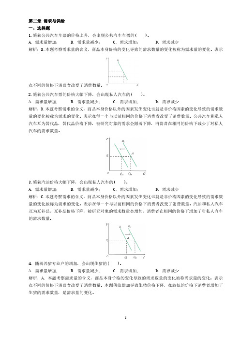
第二章需求与供给一、选择题1.随着公共汽车车票的价格上升,会出现公共汽车车票的( )。
A. 需求量增加;B. 需求量减少;C. 需求增加;D. 需求减少解析:B.本题考察需求量的含义,商品本身价格的变化导致的需求数量的变化被称为需求量的变化。
表示在不同的价格下消费者改变了消费数量。
2.随着公共汽车票的价格大幅下降,会出现私人汽车的( )。
A. 需求量增加;B. 需求量减少;C. 需求增加;D. 需求减少解析:D.本题考察需求的含义,商品本身价格以外的因素发生变化也就是非价格因素的变化导致的需求数量的变化被称为需求的变化。
表示在每一个与以前相同的价格下消费者改变了消费数量。
公共汽车和私人汽车互为替代品,替代品价格下降,被研究对象的需求会跟着下降,消费者在相同的价格下减少了对私人汽车的需求数量。
3.随着汽油价格大幅下降,会出现私人汽车的( )。
A. 需求量增加;B. 需求量减少;C. 需求增加;D. 需求减少解析:C.本题考察需求的含义,商品本身价格以外的因素发生变化也就是非价格因素的变化导致的需求数量的变化被称为需求的变化。
表示在每一个与以前相同的价格下消费者改变了消费数量。
汽油和私人汽车互为互补品,互补品价格下降,被研究对象的需求数量会增加,消费者在相同的价格下增加了对私人汽车的需求数量。
4. 随着养猪专业户的增加,会出现生猪的( )。
A. 需求量增加;B. 需求量减少;C. 需求增加;D. 需求减少解析:A. 本题考察需求量的含义,商品本身价格的变化导致的需求数量的变化被称需求量的变化。
表示在不同的价格下消费者改变了消费数量。
本题供给增加导致生猪价格下降,在较低的价格下消费者增加了生猪的需求数量,是需求量的变化。
5.随着商品房价格上升,商品房的()A.供给增加;B.供给量增加;C.供给减少;D.供给量减少。
解析:B.本题考察供给量的含义,商品本身价格的变化导致的供给数量的变化被称供给量的变化。
(完整版)微观经济学第二章课后习题答案.doc
第二章需求、供给和均衡价格1.解 :(1)将需求函数Q d= 50-5P 和供给函数Q s=-10+5P 代入均衡条件Q d=Q s , 有 :50- 5P= -10+5P 得 : Pe=6以均衡价格 Pe =6 代入需求函数Q d=50-5p , 得 : Qe=50-5 × 6或者 , 以均衡价格 Pe =6 代入供给函数Q s =-10+5P , 得 :Qe=-10+5 × 6所以 , 均衡价格和均衡数量分别为Pe =6 , Qe=20图略 .(2)将由于消费者收入提高而产生的需求函数Q d=60-5p 和原供给函数 Q s=-10+5P, 代入均衡条件 Q d= Q s有 : 60-5P=-10+5P 解得 Pe =7以均衡价格 Pe =7 代入 Q d=60-5p , 得 Qe=25或者 , 以均衡价格 Pe =7 代入 Qs =-10+5P, 得 Qe=25所以 , 均衡价格和均衡数量分别为Pe =7 , Qe=25(3)将原需求函数 Q d=50-5p 和由于技术水平提高而产生的供给函数Q s=-5+5p , 代入均衡条件 Q =Q , 有 : 50-5P=-5+5P 得 P =5.5ds e以均衡价格Pe=5.5 代入 Q d =50-5p,得 Qe=50-5× 5.5=22.5所以 , 均衡价格和均衡数量分别为Pe=5.5 ,Qe=22.5 图略。
(4)( 5)略2.解:(1)根据中点公式计算, e d=1.5(2)由于当 P=2 时, Q d=500-100*2=300,所以,有:dQ P 2 2d. ( 100)edP Q 300 3(3)作图,在 a 点 P=2 时的需求的价格点弹性为: e =GB/OG=2/3或者 e =FO/AF=2/3d d显然,利用几何方法求出P=2 时的需求的价格弹性系数和(2)中根据定义公式求出结果是相同的,都是 e d =2/33 解 :(1) 根据中点公式求得: e s 4 3(2) 由于当 P=3 时, Qs=-2+2 ×3=4 ,所以dQ P 3e s .2 1.5dP Q 4(3) 作图,在 a 点即 P=3 时的供给的价格点弹性为:e s=AB/OB=1.5显然,在此利用几何方法求出的P=3 时的供给的价格点弹性系数和(2)中根据定义公式求出的结果是相同的,都是e s=1.54.解:(1)根据需求的价格点弹性的几何方法, 可以很方便地推知 : 分别处于不同的线性需求曲线上的 a、 b、 e 三点的需求的价格点弹性是相等的, 其理由在于 , 在这三点上都有 : e d=FO/AF (2)根据求需求的价格点弹性的几何方法, 同样可以很方便地推知: 分别处于三条线性需求曲线上的 a、 e、 f 三点的需求的价格点弹性是不相等的, 且有 e da<e df <e de其理由在于 : da在 a 点有, e =GB/OG在 f 点有, e df =GC/OG在 e 点有, e de=GD/OG在以上三式中 , 由于 GB<GC<GD所以 e <e <ededa df5.解:(1)不相等。
- 1、下载文档前请自行甄别文档内容的完整性,平台不提供额外的编辑、内容补充、找答案等附加服务。
- 2、"仅部分预览"的文档,不可在线预览部分如存在完整性等问题,可反馈申请退款(可完整预览的文档不适用该条件!)。
- 3、如文档侵犯您的权益,请联系客服反馈,我们会尽快为您处理(人工客服工作时间:9:00-18:30)。
第二章需求、供给和均衡价格1. 已知某一时期某商品的需求函数为Q d=50-5P,供给函数为Q s=-10+5P。
(1)求均衡价格P e和均衡数量Q e,并作出几何图形。
(2)假定供给函数不变,由于消费者收入水平提高,使需求函数变为Q d=60-5P。
求出相应的均衡价格P e和均衡数量Q e,并作出几何图形。
(3)假定需求函数不变,由于生产技术水平提高,使供给函数变为Q s=-5+5P。
求出相应的均衡价格P e和均衡数量Q e,并作出几何图形。
(4)利用(1)、(2)和(3),说明静态分析和比较静态分析的联系和区别。
(5)利用(1)、(2)和(3),说明需求变动和供给变动对均衡价格和均衡数量的影响。
解答:(1)将需求函数Q d=50-5P和供给函数Q s=-10+5P代入均衡条件Q d=Q s,有50-5P=-10+5P得P e=6将均衡价格P e=6代入需求函数Q d=50-5P,得Q e=50-5×6=20或者,将均衡价格P e=6代入供给函数Q s=-10+5P,得Q e=-10+5×6=20所以,均衡价格和均衡数量分别为P e=6,Q e=20。
如图2—1所示。
图2—1(2)将由于消费者收入水平提高而产生的需求函数Q d=60-5P和原供给函数Q s=-10+5P代入均衡条件Q d=Q s,有60-5P=-10+5P得P e=7将均衡价格P e=7代入Q d=60-5P,得Q e=60-5×7=25或者,将均衡价格P e=7代入Q s=-10+5P,得Q e=-10+5×7=25所以,均衡价格和均衡数量分别为P e=7,Q e=25。
如图2—2所示。
图2—2(3)将原需求函数Q d=50-5P和由于技术水平提高而产生的供给函数Q s=-5+5P代入均衡条件Q d=Q s,有50-5P=-5+5P得P e=5.5将均衡价格P e=5.5代入Q d=50-5P,得Q e=50-5×5.5=22.5或者,将均衡价格P e=5.5代入Q s=-5+5P,得Q e=-5+5×5.5=22.5所以,均衡价格和均衡数量分别为P e=5.5,Q e=22.5。
如图2—3所示。
图2—3(4)所谓静态分析是考察在既定条件下某一经济事物在经济变量的相互作用下所实现的均衡状态及其特征。
也可以说,静态分析是在一个经济模型中根据给定的外生变量来求生变量的一种分析方法。
以(1)为例,在图2—1中,均衡点E就是一个体现了静态分析特征的点。
它是在给定的供求力量的相互作用下达到的一个均衡点。
在此,给定的供求力量分别用给定的供给函数Q s=-10+5P和需求函数Q d=50-5P表示,均衡点E具有的特征是:均衡价格P e=6,且当P e=6时,有Q d=Q s=Q e=20;同时,均衡数量Q e=20,且当Q e=20时,有P d =P s=P e=6。
也可以这样来理解静态分析:在外生变量包括需求函数中的参数(50,-5)以及供给函数中的参数(-10,5)给定的条件下,求出的生变量分别为P e=6和Q e=20。
依此类推,以上所描述的关于静态分析的基本要点,在(2)及图2—2和(3)及图2—3中的每一个单独的均衡点E i(i=1,2)上都得到了体现。
而所谓的比较静态分析是考察当原有的条件发生变化时,原有的均衡状态会发生什么变化,并分析比较新旧均衡状态。
也可以说,比较静态分析是考察在一个经济模型中外生变量变化时对生变量的影响,并分析比较由不同数值的外生变量所决定的生变量的不同数值,以(2)为例加以说明。
在图2—2中,由均衡点E1变动到均衡点E2就是一种比较静态分析。
它表示当需求增加即需求函数发生变化时对均衡点的影响。
很清楚,比较新、旧两个均衡点E1和E2可以看到:需求增加导致需求曲线右移,最后使得均衡价格由6上升为7,同时,均衡数量由20增加为25。
也可以这样理解比较静态分析:在供给函数保持不变的前提下,由于需求函数中的外生变量发生变化,即其中一个参数值由50增加为60,从而使得生变量的数值发生变化,其结果为,均衡价格由原来的6上升为7,同时,均衡数量由原来的20增加为25。
类似地,利用(3)及图2—3也可以说明比较静态分析方法的基本要点。
(5)由(1)和(2)可见,当消费者收入水平提高导致需求增加,即表现为需求曲线右移时,均衡价格提高了,均衡数量增加了。
由(1)和(3)可见,当技术水平提高导致供给增加,即表现为供给曲线右移时,均衡价格下降了,均衡数量增加了。
总之,一般地,需求与均衡价格成同方向变动,与均衡数量成同方向变动;供给与均衡价格成反方向变动,与均衡数量成同方向变动。
2. 假定表2—1(即教材中第54页的表2—5)是需求函数Q d=500-100P在一定价格围的需求表:表2—1价格(元) 1 2 3 4 5需求量 400 300 200 100 0(1)求出价格2元和4元之间的需求的价格弧弹性。
(2)根据给出的需求函数,求P =2元时的需求的价格点弹性。
(3)根据该需求函数或需求表作出几何图形,利用几何方法求出P =2元时的需求的价格点弹性。
它与(2)的结果相同吗?解答:(1)根据中点公式e d =-ΔQ ΔP ·P 1+P 22,Q 1+Q 22),有e d =2002·2+42,300+1002)=1.5(2)由于当P =2时,Q d=500-100×2=300,所以,有e d =-d Q d P ·P Q =-(-100)·2300=23(3)根据图2—4,在a 点即P =2时的需求的价格点弹性为e d =GB OG =200300=23或者e d =FO AF =23图2—4显然,在此利用几何方法求出的P =2时的需求的价格点弹性系数和(2)中根据定义公式求出的结果是相同的,都是e d =23。
3.假定表2—2(即教材中第54页的表2—6)是供给函数Q s=-2+2P 在一定价格围的供给表:表2—2价格(元) 2 3 4 5 6 供给量 2 4 6 8 10(1)求出价格3元和5元之间的供给的价格弧弹性。
(2)根据给出的供给函数,求P =3元时的供给的价格点弹性。
(3)根据该供给函数或供给表作出几何图形,利用几何方法求出P =3元时的供给的价格点弹性。
它与(2)的结果相同吗?解答:(1)根据中点公式e s =ΔQ ΔP ·P 1+P 22,Q 1+Q 22),有e s =42·3+52,4+82)=43(2)由于当P =3时,Q s=-2+2×3=4,所以,e s =d Q d P ·P Q =2·34=1.5。
(3)根据图2—5,在a 点即P =3时的供给的价格点弹性为e s =AB OB =64=1.5图2—5显然,在此利用几何方法求出的P =3时的供给的价格点弹性系数和(2)中根据定义公式求出的结果是相同的,都是e s =1.5。
4.图2—6(即教材中第54页的图2—28)中有三条线性的需求曲线AB 、AC 和AD 。
图2—6(1)比较a 、b 、c 三点的需求的价格点弹性的大小。
(2)比较a 、e 、f 三点的需求的价格点弹性的大小。
解答:(1)根据求需求的价格点弹性的几何方法,可以很方便地推知:分别处于三条不同的线性需求曲线上的a 、b 、c 三点的需求的价格点弹性是相等的。
其理由在于,在这三点上,都有e d =FO AF(2)根据求需求的价格点弹性的几何方法,同样可以很方便地推知:分别处于三条不同的线性需求曲线上的a 、e 、f 三点的需求的价格点弹性是不相等的,且有e a d <e f d <e ed 。
其理由在于在a 点有:e ad =GB OG在f 点有:e fd =GC OG在e 点有:e ed =GD OG在以上三式中,由于GB <GC <GD ,所以,e a d <e f d <e ed 。
5.利用图2—7(即教材中第55页的图2—29)比较需求价格点弹性的大小。
(1)图(a )中,两条线性需求曲线D 1和D 2相交于a 点。
试问:在交点a ,这两条直线型的需求的价格点弹性相等吗?(2)图(b)中,两条曲线型的需求曲线D 1和D 2相交于a 点。
试问:在交点a ,这两条曲线型的需求的价格点弹性相等吗?图2—7解答:(1)因为需求的价格点弹性的定义公式为e d =-d Q d P ·PQ,因为在图(a )中,需求曲线D 1的-d Q d P 值大于需求曲线D 2的-d Qd P值,所以,在两条线性需求曲线D 1和D 2的交点a ,在P和Q 给定的前提下,需求曲线D 1的弹性大于需求曲线D 2的弹性。
(2)因为需求的价格点弹性的定义公式为e d =-d Q d P ·P Q ,此公式中的-d Qd P项是需求曲线某一点的斜率的绝对值的倒数,而曲线型需求曲线上某一点的斜率可以用过该点的切线的斜率来表示。
在图(b )中,需求曲线D 1过a 点的切线AB 的斜率的绝对值小于需求曲线D 2过a 点的切线FG 的斜率的绝对值,所以,根据在解答(1)中的道理可推知,在交点a ,在P 和Q 给定的前提下,需求曲线D 1的弹性大于需求曲线D 2的弹性。
6.假定某消费者关于某种商品的消费数量Q 与收入M 之间的函数关系为M =100Q 2。
求:当收入M =6400时的需求的收入点弹性。
解答:由已知条件M =100Q 2,可得Q =M 100于是,有d Q d M =12⎝ ⎛⎭⎪⎫M 100-12·1100进一步,可得e M =d Q d M ·M Q=12⎝ ⎛⎭⎪⎫M 100-12·1100·100·⎝ ⎛⎭⎪⎫M 1002M 100=12观察并分析以上计算过程及其结果,可以发现,当收入函数M =aQ 2(其中a >0,为常数)时,则无论收入M 为多少,相应的需求的收入点弹性恒等于12。
7.假定需求函数为Q =MP -N,其中M 表示收入,P 表示商品价格,N(N >0)为常数。
求:需求的价格点弹性和需求的收入点弹性。
解答:由已知条件Q =MP -N,可得e d =-d Q d P ·P Q =-M·(-N)·P -N -1·P MP -N =Ne M =d Q d M ·M Q =P -N ·MMP -N =1由此可见,一般地,对于幂指数需求函数Q(P)=MP -N而言, 其需求的价格点弹性总等于幂指数的绝对值N 。
而对于线性需求函数Q(M)=MP -N而言,其需求的收入点弹性总是等于1。