2020161自动控制原理(中英文)
自动控制原理(中英文)
自动控制原理(中英文)《自动控制原理》课程教学大纲课程编号:2020161课程类别:必修授课对象:本科三年级先修课程:复变函数,积分变换,信号与系统。
学分:4总学时:56 课内学时:48实验学时: 8一、课程性质、教学目得与任务课程性质:专业基础课,专业知识链条中得关键环节之一,自动控制原理就是仪器仪表类、测控类专业得重要基础课之一,这些专业主要学习信号传感(获取)、信号处理、控制及光机电系统等知识,而控制就是知识链条中得重要一环,随着科技发展,自动化、智能化已成为仪器、产品、系统等得重要功能,这就要求学生必须具备自动控制方面得知识。
教学目得与任务:培养学生自动控制原理得基础知识,学习掌握经典控制得基本理论、基本方法与控制系统得基本设计方法,重点学习分析与设计线性控制系统得基本理论、基本方法及控制系统设计方法.主要内容包括:控制系统得数学模型、控制系统得时域分析法、控制系统得根轨迹法、控制系统得频域分析法、控制系统得常用校正方法等。
二、教学基本要求学习经典控制得基本理论与基本方法,重点学习分析与设计线性控制系统得基本理论与基本方法。
主要内容包括:控制系统得数学模型、控制系统得时域分析法、控制系统得根轨迹法、控制系统得频域分析法、控制系统得常用校正方法等。
三、教学内容第一章控制系统得一般要概念 (4课时)自动控制得基本原理与方式,自动控制系统示例,自动控制系统得分类,对自动控制系统得基本要求1、基本概念;2、反馈系统基本组成;3、基本控制方式;4、控制系统分类:开环、闭环、复合控制;第二章控制系统得数学模型 (8课时)控制系统得时域数学模型,拉普拉斯变换,控制系统得复域数学模型,控制系统得状态空间模型,控制系统得结构图与信号流图2-1时域模型、微分方程表示方法;2-2 复域模型1、传递函数得定义与性质;2、传递函数得零、极点表示,开环增益、根轨迹增益等;3、典型环节得传递函数(比例、惯性、微分、积分、振荡);2-3 控制系统得结构图与信号流图1、结构图得等效变换与化简2、信号流图组成与性质A.性质、术语(理解)B。
自动控制原理英文版课后全部_答案

Module3Problem 3.1(a) When the input variable is the force F. The input variable F and the output variable y are related by the equation obtained by equating the moment on the stick:2.233y dylF lk c l dt=+Taking Laplace transforms, assuming initial conditions to be zero,433k F Y csY =+leading to the transfer function31(4)Y k F c k s=+ where the time constant τ is given by4c kτ=(b) When F = 0The input variable is x, the displacement of the top point of the upper spring. The input variable x and the output variable y are related by the equation obtained by the moment on the stick:2().2333y y dy k x l kl c l dt-=+Taking Laplace transforms, assuming initial conditions to be zero,3(24)kX k cs Y =+leading to the transfer function321(2)Y X c k s=+ where the time constant τ is given by2c kτ=Problem 3.2 P 54Determine the output of the open-loop systemG(s) = 1asT+to the inputr(t) = tSketch both input and output as functions of time, and determine the steady-state error between the input and output. Compare the result with that given by Fig3.7 . Solution :While the input r(t) = t , use Laplace transforms, Input r(s)=21sOutput c(s) = r(s) G(s) = 2(1)aTs s ⋅+ = 211T T a s s Ts ⎛⎫ ⎪-+ ⎪ ⎪+⎝⎭the time-domain response becomes c(t) = ()1t Tat aT e ---Problem 3.33.3 The massless bar shown in Fig.P3.3 has been displaced a distance 0x and is subjected to a unit impulse δ in the direction shown. Find the response of the system for t>0 and sketch the result as a function of time. Confirm the steady-state response using the final-value theorem. Solution :The equation obtained by equating the force:00()kx cxt δ+=Taking Laplace transforms, assuming initial condition to be zero,K 0X +Cs 0X =1leading to the transfer function()XF s =1K Cs +=1C1K s C+The time-domain response becomesx(t)=1CC tK e -The steady-state response using the final-value theorem:lim ()t x t →∞=0lim s →s 1K Cs +1s =1K00000()()()1;11111()K t CK x x Cx t Kx X K Cs Kx Kx X C Cs K K s KKx x t eCδ-++=⇒++=--∴==⋅++-=⋅According to the final-value theorem:0001lim ()lim lim 01t s s Kx sx t s X C K s K→∞→→-=⋅=⋅=+ Problem 3.4 Solution:1.If the input is a unit step, then1()R s s=()()11R s C s sτ−−−→−−−→+ leading to,1()(1)C s s sτ=+taking the inverse Laplace transform gives,()1tc t e τ-=-as the steady-state output is said to have been achieved once it is within 1% of the final value, we can solute ―t‖ like this,()199%1tc t e τ-=-=⨯ (the final value is 1) hence,0.014.60546.05te t sττ-==⨯=(the time constant τ=10s)2.the numerical value of the numerator of the transfer function doesn’t affect the answer. See this equation, If ()()()1C s AG s R s sτ==+ then()(1)A C s s sτ=+giving the time-domain response()(1)tc t A e τ-=-as the final value is A, the steady-state output is achieved when,()(1)99%tc t A e A τ-=-=⨯solute the equation, t=4.605τ=46.05sthe result make no different from that above, so we said that the numerical value of the numerator of the transfer function doesn’t affect the answer.If a<1, as the time increase, the two lines won`t cross. In the steady state the output lags the input by a time by more than the time constant T. The steady error will be negative infinite.R(t)C(t)Fig 3.7 tR(t)C(t)tIf a=1, as the time increase, the two lines will be parallel. It is as same as Fig 3.7.R(t)C(t)tIf a>1, as the time increase, the two lines will cross. In the steady state the output lags the input by a time by less than the time constant T.The steady error will be positive infinite.Problem 3.5 Solution: R(s)=261s s+, Y(s)=26(51)s s s +⋅+=229614551s s s -+++ /5()62929t y t t e -∴=-+so the steady-state error is 29(-30). To conform the result:5lim ()lim(62929);tt t y t t -→∞→∞=-+=∞6lim ()lim ()lim ()lim(51)t s s s s y t y s Y s s s →∞→→→+====∞+.20lim ()lim ()lim [()()]161lim [()1]()lim (1)()5130ss t s s s s e e t S E S S Y S R S S G S R S S S S S→∞→→→→==⋅=⋅-=⋅-=⋅-⋅++=- Therefore, the solution is basically correct.Problem 3.623yy x += since input is of constant amplitude and variable frequency , it can be represented as:j tX eA ω=as we know ,the output should be a sinusoidal signal with the same frequency of the input ,it can also be represented as:R(t)C(t)t0j t y y e ω=hence23j tj tj tj yyeeeA ωωωω+=00132j y Aω=+ 0294Ayω=+ 2tan3w ϕ=- Its DC(w→0) value is 003Ay ω==Requirement 01122w yy==21123294AA ω=⨯+ →32w = while phase lag of the input:1tan 14πϕ-=-=-Problem 3.7One definition of the bandwidth of a system is the frequency range over which the amplitude of the output signal is greater than 70% of the input signal amplitude when a system is subjected to a harmonic input. Find a relationship between the bandwidth and the time constant of a first-order system. What is the phase angle at the bandwidth frequency ? Solution :From the equation 3.41000.71r A r ωτ22=≥+ (1)and ω≥0 (2) so 1.020ωτ≤≤so the bandwidth 1.02B ωτ=from the equation 3.43the phase angle 110tan tan 1.024c πωτ--∠=-=-=Problem 3.8 3.8 SolutionAccording to generalized transfer function of First-Order Feedback Systems11C KG K RKGHK sτ==+++the steady state of the output of this system is 2.5V .∴if s →0, 2.51104C R→=. From this ,we can get the value of K, that is 13K =.Since we know that the step input is 10V , taking Laplace transforms,the input is 10S.Then the output is followed1103()113C s S s τ=⨯++Taking reverse Laplace transforms,4/4332.5 2.5 2.5(1)t t C e eττ--=-=-From the figure, we can see that when the time reached 3s,the value of output is 86% of the steady state. So we can know34823(2)*4393τττ-=-⇒-=-⇒=, 4/3310.8642t t e ττ-=-=⇒=The transfer function is3128s +146s+Let 12+8s=0, we can get the pole, that is 1.5s =-2/3- Problem 3.9 Page 55 Solution:The transfer function can be represented,()()()()()()()o o m i m i v s v s v s G s v s v s v s ==⋅While,()1()111//()()11//o m m i v s v s sRCR v s sC sC v s R R sC sC =+⎛⎫+ ⎪⎝⎭=⎡⎤⎛⎫++ ⎪⎢⎥⎝⎭⎣⎦Leading to the final transfer function,21()13()G s sRC sRC =++ And the reason:the second simple lag compensation network can be regarded as the load of the first one, and according to Load Effect , the load affects the primary relationship; so the transfer function of the comb ination doesn’t equal the product of the two individual lag transfer functio nModule4Problem4.14.1The closed-loop transfer function is10(6)102(6)101610S S S S C RS s +++++==Comparing with the generalized second-order system,we getProblem4.34.3Considering the spring rise x and the mass rise y. Using Newton ’s second law of motion..()()d x y m y K x y c dt-=-+Taking Laplace transforms, assuming zero initial conditions2mYs KX KY csX csY =-+-resulting in the transfer funcition where2Y cs K X ms cs K +=++ And521.26*10cmkc ζ== Problem4.4 Solution:The closed-loop transfer function is210263101011n n d n W EW E W W E ====-=2121212K C K S S K R S S K S S ∙+==+++∙+Comparing the closed-loop transfer function with the generalized form,2222n n nCR s s ωξωω=++ it is seen that2n K ω= And that22n ξω= ; 1Kξ=The percentage overshoot is therefore21100PO eξπξ--=11100k keπ-∙-=Where 10%PO ≤When solved, gives 1.2K ≤(2.86)When K takes the value 1.2, the poles of the system are given by22 1.20s s ++=Which gives10.45s j =-±±s=-1 1.36jProblem4.5ReIm0.45-0.45-14.5 A unity-feedback control system has the forward-path transfer functionG (s) =10)S(s K+Find the closed-loop transfer function, and develop expressions for the damping ratio And damped natural frequency in term of K Plot the closed-loop poles on the complex Plane for K = 0,10,25,50,100.For each value of K calculate the corresponding damping ratio and damped natural frequency. What conclusions can you draw from the plot?Solution: Substitute G(s)=(10)K s s + into the feedback formula : Φ(s)=()1()G S HG S +.And in unitfeedback system H=1. Result in: Φ(s)=210Ks s K++ So the damped natural frequencyn ω=K ,damping ratio ζ=102k =5k.The characteristic equation is 2s +10S+K=0. When K ≤25,s=525K -±-; While K>25,s=525i K -±-; The value ofn ω and ζ corresponding to K are listed as follows.K 0 10 25 50 100 Pole 1 1S 0 515-+ -5 -5+5i 553i -+Pole 2 2S -10 515-- -5 -5-5i553i --n ω 010 5 52 10 ζ ∞2.51 0.5 0.5Plot the complex plane for each value of K:We can conclude from the plot.When k ≤25,poles distribute on the real axis. The smaller value of K is, the farther poles is away from point –5. The larger value of K is, the nearer poles is away from point –5.When k>25,poles distribute away from the real axis. The smaller value of K is, the further (nearer) poles is away from point –5. The larger value of K is, the nearer (farther) poles is away from point –5.And all the poles distribute on a line parallels imaginary axis, intersect real axis on the pole –5.Problem4.61tb b R L C b o v dv i i i i v dt C R L dt=++=++⎰Taking Laplace transforms, assuming zero initial conditions, reduces this equation to011b I Cs V R Ls ⎛⎫=++ ⎪⎝⎭20b V RLs I Ls R RLCs =++ Since the input is a constant current i 0, so01I s=then,()2b RLC s V Ls R RLCs==++ Applying the final-value theorem yields ()()0lim lim 0t s c t sC s →∞→==indicating that the steady-state voltage across the capacitor C eventually reaches the zero ,resulting in full error.Problem4.74.7 Prove that for an underdamped second-order system subject to a step input, thepercentage overshoot above the steady-state output is a function only of the damping ratio .Fig .4.7SolutionThe output can be given by222222()(2)21()(1)n n n n n n C s s s s s s s ωζωωζωζωωζ=+++=-++- (1)the damped natural frequencyd ω can be defined asd ω=21n ωζ- (2)substituting above results in22221()()()n n n d n d s C s s s s ζωζωζωωζωω+=--++++ (3) taking the inverse transform yields22()1sin()11tan n t d e c t t where ζωωφζζφζ-=-+--=(4)the maximum output is22()1sin()11n t p d p p d n e c t t t ζωωφζππωωζ-=-+-==-(5)so the maximum is2/1()1p c t eπζζ--=+the percentage overshoot is therefore2/1100PO eπζζ--=Problem4.8 Solution to 4.8:Considering the mass m displaced a distance x from its equilibrium position, the free-body diagram of the mass will be as shown as follows.aP cdx kxkxmUsing Newton ’s second law of motion,22p k x c x mx m x c x k x p--=++=Taking Laplace transforms, assuming zero initial conditions,2(2)X ms cs k P ++= results in the transfer function2/(1/)/((/)2/)X P m s c m s k m =++ 2(2/)(2/)((/)2/)k k m s c m s k m =++As we see2(2)X m s c s k P++= As P is constantSo X ∝212ms cs k ++ . When 56.25102cs m-=-=-⨯ ()25min210mscs k ++=4max5100.110X == This is a second-order transfer function where 22/n k m ω= and/2/22n c w m c k m ζ== The damped natural frequency is given by 2212/1/8d n k m c km ωωζ=-=-22/(/2)k m c m =- Using the given data,462510/2100.050.2236n ω=⨯⨯⨯== 462502.79501022100.05ζ-==⨯⨯⨯⨯ ()240.22361 2.7950100.2236d ω-=⨯-⨯= With these data we can draw a picture14.0501160004.673600p de s e T T πωτζωτ======222222112/1222()22,,,428sin (sin cos )0tan 7.030.02n n pp dd n dd n ntd d t t t n d p d d p ddd p p p nX k m c k P ms cs k k m s s s m m k c k c cm m m m km p x e tm p xe t t m t t x m ζωζωωωζωωωωζζωωωζωωωωωωωζω--===⋅=⋅++++++=-===∴==-+=∴=⇒=⇒= 其中Problem4.10 4.10 solution:The system is similar to the one in the book on PAGE 58 to PAGE 63. The difference is the connection of the spring. So the transfer function is2222l n d n n w s w s w θθζ=++222(),;p a m ld a m p m l m l l m mm l lk k k N RJs RCs R k k N k J N J J C N c c N N N θθωθωθ=+++=+=+===p a mn K K K w NJ R='damping ratio 2p a m c NRK K K J ζ='But the value of J is different, because there is a spring connected.122s m J J J J N N '=++Because of final-value theorem,2l nd w θθζ=Module5Problem5.45.4 The closed-loop transfer function of the system may be written as2221010(1)610101*********CR K K K S S K K S S K S S +++==+++++++ The closed-loop poles are the solutions of the characteristic equation6364(1010)3110210(1)n K S K JW K -±-+==-±+=+ 210(1)6310(1)E K E K +==+In order to study the stability of the system, the behavior of the closed-loop poles when the gain K increases from zero to infinte will be observed. So when12K = 3010E =321S J =-± 210K = 3110110E =3101S J =-± 320K = 21070E =3201S J =-±双击下面可以看到原图ReProblem5.5SolutionThe closed-loop transfer function is2222(1)1(1)KC K KsKR s K as s aKs Kass===+++++∙+Comparing the closed-loop transfer function with the generalized form, 2222nn nCR s sωξωω=++Leading to2nKa Kωξ==The percentage overshoot is therefore2110040%PO eξπξ--==Producing the result0.869ξ=(0.28)And the peak time241PnT sπωξ==-Leading to1.586nω=(0.82)Problem5.75.7 Prove that the rise time T r of a second-order system with a unit step input is given byT r = d ω1 tan -1n dζωω = d ω1 tan -1d ωζ21--Plot the rise against the damping ratio.Solution:According to (4.33):c(t)=1-2(cos sin )1n t d d e t t ζωζωωζ-+-. 4.33When t=r T ,c(t)=1.substitue c(t)= 1 into (4.33) Producing the resultr T =d ω1 tan -1n dζωω = d ω1 tan -112ζζ--Plot the rise time against the damping ratio:Problem5.9Solution to 5.9:As we know that the system is the open-loop transfer function of a unity-feedback control system.So ()()GH S G S = Given as()()()425KGH s s s =-+The close-loop transfer function of the system may be written as()()()()()41254G s C Ks R GH s s s K ==+-++ The characteristic equation is()()2254034100s s K s s K -++=⇒++-=According to the Routh ’s method, the Routh ’s array must be formed as follow20141030410s K s s K -- For there is no closed-loop poles to the right of the imaginary axis4100 2.5K K -≥⇒≥ Given that 0.5ζ=4103 4.752410n K K K ωζ=-=⇒=- When K=0, the root are s=+2,-5According to the characteristic equation, the solutions are349424s K =-±-while 3.0625K ≤, we have one or two solutions, all are integral number.Or we will have solutions with imaginary number. So we can drawK=102 -5 K=0K=3.0625K=2.5 K=10Open-loop polesClosed-loop polesProblem5.10 5.10 solution:0.62/n w rad sζ==according to()211sin()21n w t d e c w t ζφζ-=-+=- 1.2sin(1.6)0.4t e t φ-⋅+= 4t a n3φ= finally, t is delay time:1.23t s ≈(0.67)Module6Problem 6.3First we assume the disturbance D to be zero:e R C =-1011C K e s s =⋅⋅⋅+Hence:(1)10(1)e s s R K s s +=++ Then we set the input R to be zero:10()(1)C K e D e s s =⋅+⋅=-+ ⇒ 1010(1)e D K s s =-++Adding these two results together:(1)1010(1)10(1)s s e R D K s s K s s +=⋅-⋅++++21()R s s =; 1()D s s= ∴222110910(1)10(1)100(1)s s e Ks s s Ks s s s s s +-=-=++++++ the steady-state error:232200099lim lim lim 0.09100100ss s s s s s s e s e s s s s s →→→--=⋅===-++++Problem 6.4Determine the disturbance rejection ratio(DRR) for the system shown in Fig P.6.4+fig.P.6.4 solution :from the diagram we can know :0.210.05mv K RK c === so we can get that()0.21115()0.05v m m OL n CL K K DRR cR ωω∆⨯==+=+=∆210.10.050.050.025s s =++, so c=0.025, DRR=9Problem 6.5 6.5 SolutionFor the purposes of determining the steady-state error of the system, we should get to know the effect of the input and the disturbance along when the other will be assumed to be zero.First to simplify the block diagram to the following patter:110s +2021Js Tddθoθ0.220.10.05s ++__+d T—Allowing the transfer function from the input to the output position to be written as01220220d Js s θθ=++ 012222020240*220220(220)dJs s Js s s Js s sθθ===++++++ According to the equation E=R-C:022*******(2)()lim[()()]lim[(1)]lim 0.2220220ssr d s s s Js e s s s s Js s Js s δδδθθ→→→+=-=-==++++问题;1. 系统型为2,对于阶跃输入,稳态误差为0.2. 终值定理写的不对。
《自动控制原理B(双语)》课程简介和教学大纲.doc

自动控制原理(B)课程简介课程编号:15J8047课程名称:(中文)自动控制原理(B)(英文)Introduction to Automatic Control学分/学时:42学时,实验6学时开课学期:秋季先修课程:高等数学、工程数学、大学物理内容简介:(500字以内)《自动控制原理》属于技术科学,是为专业课学习和参加控制工程实践而设置的,研究的对象是自动控制系统,研究的中心问题是控制系统在控制过程中的性能,学科的基本内容分为数学模型、工程分析计算方法和系统一般规律三个部分。
要求学生能够正确地理解和运用课程的基本概念及基本理论,逐步掌握“定性分析、定量估算和仿真实验"的研究问题的方法。
本课程内容主要为经典控制中的线性理论,课程前后内容联系紧密、系统性强,所附加的实验课,以学习控制系统的基本实验方法和培养测试、分析能力为主。
自动控制原理(B)课程教学大纲课程编号:15J8047课程名称:(中文)自动控制原理(B)(英文)Introduction to Automatic Control学分/学时:42学时,实验6学时先修课程:高等数学、工程数学、大学物理课程教学目标课程的性质:本科专业基本课,为必修课目的和任务:本课程是研究自动控制系统规律性的一门工程学科,是重要的专业基本课程。
通过本课程的教学工作,要求学生能够正确地理解和运用课程的基本概念和理论,逐步掌握“定性分析、定量估算和仿真实验”的研究问题的方法,具有从事与飞行器自动控制系统有■关的丁程实践与理论研究的基本知识,并为进一步学习现代控制理论打下基本。
教学内容及基本要求第一章自动控制的一般概念(2学时)1.1自动控制的任务1.2自动控制的基本方式1.3自动控制系统示例1.4对控制系统的性能要求第二章自动控制系统的数学模型(8学时)2.1控制系统微分方程的建立2.2非线性微分方程的线性化2.3拉普拉斯变换2.4传递函数2.5动态结构图2.6结构图的等效变换2.7典型反馈系统的几种传递函数第三章时域分析法(8学时)3.1典型响应及性能指标3.2 一、二阶系统分析3.3二阶系统分析3.4系统稳态误差分析及计算第四章根轨迹法(6学时)4.1根轨迹与根轨迹方程4.2根轨迹的绘制法则4.3系统闭环零、极点分布与阶跃响应的关系4.4系统阶跃响应的根轨迹分析第五章频率法(8学时)5.1频率特性5.2典型环节的频率特性5.3开环系统的频率特性5.4频率稳定判据5.5系统闭环频率特性与阶跃响应的关系5.5开环频率特性与系统阶跃响应的关系第六章控制系统的校正方法(4学时)6.1系统校正设计基础6.2串联校正6.3串联校正的理论设计方法6.4反馈校正6.5复合校正第七章状态空间分析方法(6学时)7.1状态空间方法基础7.2线性系统的可控性和可观测性7.3状态反馈与状态观测器7.4有界输入、有界输出稳定性7.5李雅普诺夫第二方法.教学安排及方式学时分配:讲课实验习题课第一章21第二章82第三章821第四章61第五章821第六章421第七章6课内外学时比:1:1.5实验安排:共三次实验,每次二小时。
《自动控制原理》试卷及答案(英文10套)
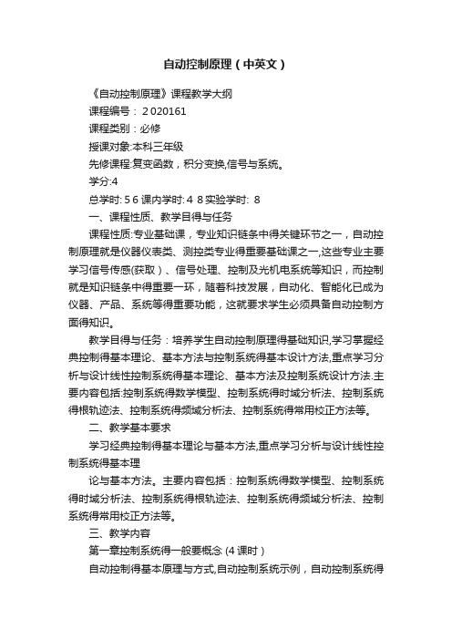
AUTOMATIC CONTROL THEOREM (1)⒈ Derive the transfer function and the differential equation of the electric network⒉ Consider the system shown in Fig.2. Obtain the closed-loop transfer function)()(S R S C , )()(S R S E . (12%) ⒊ The characteristic equation is given 010)6(5)(123=++++=+K S K S S S GH . Discuss the distribution of the closed-loop poles. (16%)① There are 3 roots on the LHP ② There are 2 roots on the LHP② There are 1 roots on the LHP ④ There are no roots on the LHP . K=?⒋ Consider a unity-feedback control system whose open-loop transfer function is )6.0(14.0)(++=S S S S G . Obtain the response to a unit-step input. What is the rise time for this system? What is the maximum overshoot? (10%)Fig.15. Sketch the root-locus plot for the system )1()(+=S S K S GH . ( The gain K is assumed to be positive.)① Determine the breakaway point and K value.② Determine the value of K at which root loci cross the imaginary axis.③ Discuss the stability. (12%)6. The system block diagram is shown Fig.3. Suppose )2(t r +=, 1=n . Determine the value of K to ensure 1≤e . (12%)Fig.37. Consider the system with the following open-loop transfer function:)1)(1()(21++=S T S T S K S GH . ① Draw Nyquist diagrams. ② Determine the stability of the system for two cases, ⑴ the gain K is small, ⑵ K is large. (12%)8. Sketch the Bode diagram of the system shown in Fig.4. (14%)⒈212121121212)()()(C C S C C R R C S C C R S V S V ++++=⒉ 2423241321121413211)()(H G H G G G G G G G H G G G G G G G S R S C ++++++=⒊ ① 0<K<6 ② K ≤0 ③ K ≥6 ④ no answer⒋⒌①the breakaway point is –1 and –1/3; k=4/27 ② The imaginary axis S=±j; K=2③⒍5.75.3≤≤K⒎ )154.82)(181.34)(1481.3)(1316.0()11.0(62.31)(+++++=S S S S S S GHAUTOMATIC CONTROL THEOREM (2)⒈Derive the transfer function and the differential equation of the electric network⒉ Consider the equation group shown in Equation.1. Draw block diagram and obtain the closed-loop transfer function )()(S R S C . (16% ) Equation.1 ⎪⎪⎩⎪⎪⎨⎧=-=-=--=)()()()()]()()([)()]()()()[()()()]()()[()()()(3435233612287111S X S G S C S G S G S C S X S X S X S G S X S G S X S C S G S G S G S R S G S X⒊ Use Routh ’s criterion to determine the number of roots in the right-half S plane for the equation 0400600226283)(12345=+++++=+S S S S S S GH . Analyze stability.(12% )⒋ Determine the range of K value ,when )1(2t t r ++=, 5.0≤SS e . (12% )Fig.1⒌Fig.3 shows a unity-feedback control system. By sketching the Nyquist diagram of the system, determine the maximum value of K consistent with stability, and check the result using Routh ’s criterion. Sketch the root-locus for the system (20%)(18% )⒎ Determine the transfer function. Assume a minimum-phase transfer function.(10% )⒈1)(1)()(2122112221112++++=S C R C R C R S C R C R S V S V⒉ )(1)()(8743215436324321G G G G G G G G G G G G G G G G S R S C -+++=⒊ There are 4 roots in the left-half S plane, 2 roots on the imaginary axes, 0 root in the RSP. The system is unstable.⒋ 208<≤K⒌ K=20⒍⒎ )154.82)(181.34)(1481.3)(1316.0()11.0(62.31)(+++++=S S S S S S GHAUTOMATIC CONTROL THEOREM (3)⒈List the major advantages and disadvantages of open-loop control systems. (12% )⒉Derive the transfer function and the differential equation of the electric network⒊ Consider the system shown in Fig.2. Obtain the closed-loop transfer function)()(S R S C , )()(S R S E , )()(S P S C . (12%)⒋ The characteristic equation is given 02023)(123=+++=+S S S S GH . Discuss the distribution of the closed-loop poles. (16%)5. Sketch the root-locus plot for the system )1()(+=S S K S GH . (The gain K is assumed to be positive.)④ Determine the breakaway point and K value.⑤ Determine the value of K at which root loci cross the imaginary axis. ⑥ Discuss the stability. (14%)6. The system block diagram is shown Fig.3. 21+=S K G , )3(42+=S S G . Suppose )2(t r +=, 1=n . Determine the value of K to ensure 1≤SS e . (15%)7. Consider the system with the following open-loop transfer function:)1)(1()(21++=S T S T S K S GH . ① Draw Nyquist diagrams. ② Determine the stability of the system for two cases, ⑴ the gain K is small, ⑵ K is large. (15%)⒈ Solution: The advantages of open-loop control systems are as follows: ① Simple construction and ease of maintenance② Less expensive than a corresponding closed-loop system③ There is no stability problem④ Convenient when output is hard to measure or economically not feasible. (For example, it would be quite expensive to provide a device to measure the quality of the output of a toaster.)The disadvantages of open-loop control systems are as follows:① Disturbances and changes in calibration cause errors, and the output may be different from what is desired.② To maintain the required quality in the output, recalibration is necessary from time to time.⒉ 1)(1)()()(2122112221122112221112+++++++=S C R C R C R S C R C R S C R C R S C R C R S U S U ⒊351343212321215143211)()(H G G H G G G G H G G H G G G G G G G G S R S C +++++= 35134321232121253121431)1()()(H G G H G G G G H G G H G G H G G H G G G G S P S C ++++-+=⒋ R=2, L=1⒌ S:①the breakaway point is –1 and –1/3; k=4/27 ② The imaginary axis S=±j; K=2⒍5.75.3≤≤KAUTOMATIC CONTROL THEOREM (4)⒈ Find the poles of the following )(s F :se s F --=11)( (12%)⒉Consider the system shown in Fig.1,where 6.0=ξ and 5=n ωrad/sec. Obtain the rise time r t , peak time p t , maximum overshoot P M , and settling time s t when the system is subjected to a unit-step input. (10%)⒊ Consider the system shown in Fig.2. Obtain the closed-loop transfer function)()(S R S C , )()(S R S E , )()(S P S C . (12%)⒋ The characteristic equation is given 02023)(123=+++=+S S S S GH . Discuss the distribution of the closed-loop poles. (16%)5. Sketch the root-locus plot for the system )1()(+=S S K S GH . (The gain K is assumed to be positive.)⑦ Determine the breakaway point and K value.⑧ Determine the value of K at which root loci cross the imaginary axis.⑨ Discuss the stability. (12%)6. The system block diagram is shown Fig.3. 21+=S K G , )3(42+=S S G . Suppose )2(t r +=, 1=n . Determine the value of K to ensure 1≤SS e . (12%)7. Consider the system with the following open-loop transfer function:)1)(1()(21++=S T S T S K S GH . ① Draw Nyquist diagrams. ② Determine the stability of the system for two cases, ⑴ the gain K is small, ⑵ K is large. (12%)8. Sketch the Bode diagram of the system shown in Fig.4. (14%)⒈ Solution: The poles are found from 1=-s e or 1)sin (cos )(=-=-+-ωωσωσj e e j From this it follows that πωσn 2,0±== ),2,1,0( =n . Thus, the poles are located at πn j s 2±=⒉Solution: rise time sec 55.0=r t , peak time sec 785.0=p t ,maximum overshoot 095.0=P M ,and settling time sec 33.1=s t for the %2 criterion, settling time sec 1=s t for the %5 criterion.⒊ 351343212321215143211)()(H G G H G G G G H G G H G G G G G G G G S R S C +++++= 35134321232121253121431)1()()(H G G H G G G G H G G H G G H G G H G G G G S P S C ++++-+=⒋R=2, L=15. S:①the breakaway point is –1 and –1/3; k=4/27 ② The imaginary axis S=±j; K=2⒍5.75.3≤≤KAUTOMATIC CONTROL THEOREM (5)⒈ Consider the system shown in Fig.1. Obtain the closed-loop transfer function )()(S R S C , )()(S R S E . (18%)⒉ The characteristic equation is given 0483224123)(12345=+++++=+S S S S S S GH . Discuss the distribution of the closed-loop poles. (16%)⒊ Sketch the root-locus plot for the system )15.0)(1()(++=S S S K S GH . (The gain K is assumed to be positive.)① Determine the breakaway point and K value.② Determine the value of K at which root loci cross the imaginary axis. ③ Discuss the stability. (18%)⒋ The system block diagram is shown Fig.2. 1111+=S T K G , 1222+=S T K G . ①Suppose 0=r , 1=n . Determine the value of SS e . ②Suppose 1=r , 1=n . Determine the value of SS e . (14%)⒌ Sketch the Bode diagram for the following transfer function. )1()(Ts s K s GH +=, 7=K , 087.0=T . (10%)⒍ A system with the open-loop transfer function )1()(2+=TS s K S GH is inherently unstable. This system can be stabilized by adding derivative control. Sketch the polar plots for the open-loop transfer function with and without derivative control. (14%)⒎ Draw the block diagram and determine the transfer function. (10%)⒈∆=321)()(G G G S R S C ⒉R=0, L=3,I=2⒋①2121K K K e ss +-=②21211K K K e ss +-= ⒎11)()(12+=RCs s U s UAUTOMATIC CONTROL THEOREM (6)⒈ Consider the system shown in Fig.1. Obtain the closed-loop transfer function )()(S R S C , )()(S R S E . (18%)⒉The characteristic equation is given 012012212010525)(12345=+++++=+S S S S S S GH . Discuss thedistribution of the closed-loop poles. (12%)⒊ Sketch the root-locus plot for the system )3()1()(-+=S S S K S GH . (The gain K is assumed to be positive.)① Determine the breakaway point and K value.② Determine the value of K at which root loci cross the imaginary axis. ③ Discuss the stability. (15%)⒋ The system block diagram is shown Fig.2. SG 11=, )125.0(102+=S S G . Suppose t r +=1, 1.0=n . Determine the value of SS e . (12%)⒌ Calculate the transfer function for the following Bode diagram of the minimum phase. (15%)⒍ For the system show as follows, )5(4)(+=s s s G ,1)(=s H , (16%) ① Determine the system output )(t c to a unit step, ramp input.② Determine the coefficient P K , V K and the steady state error to t t r 2)(=.⒎ Plot the Bode diagram of the system described by the open-loop transfer function elements )5.01()1(10)(s s s s G ++=, 1)(=s H . (12%)w⒈32221212321221122211)1()()(H H G H H G G H H G G H G H G H G G G S R S C +-++-+-+= ⒉R=0, L=5 ⒌)1611()14)(1)(110(05.0)(2s s s s s s G ++++= ⒍t t e e t c 431341)(--+-= t t e e t t c 41213445)(---+-= ∞=P K , 8.0=V K , 5.2=ss eAUTOMATIC CONTROL THEOREM (7)⒈ Consider the system shown in Fig.1. Obtain the closed-loop transfer function)()(S R S C , )()(S R S E . (16%)⒉ The characteristic equation is given 01087444)(123456=+--+-+=+S S S S S S S GH . Discuss the distribution of the closed-loop poles. (10%)⒊ Sketch the root-locus plot for the system 3)1()(S S K S GH +=. (The gain K is assumed to be positive.)① Determine the breakaway point and K value.② Determine the value of K at which root loci cross the imaginary axis. ③ Discuss the stability. (15%)⒋ Show that the steady-state error in the response to ramp inputs can be made zero, if the closed-loop transfer function is given by:nn n n n n a s a s a s a s a s R s C +++++=---1111)()( ;1)(=s H (12%)⒌ Calculate the transfer function for the following Bode diagram of the minimum phase.(15%)w⒍ Sketch the Nyquist diagram (Polar plot) for the system described by the open-loop transfer function )12.0(11.0)(++=s s s S GH , and find the frequency and phase such that magnitude is unity. (16%)⒎ The stability of a closed-loop system with the following open-loop transfer function )1()1()(122++=s T s s T K S GH depends on the relative magnitudes of 1T and 2T . Draw Nyquist diagram and determine the stability of the system.(16%) ( 00021>>>T T K )⒈3213221132112)()(G G G G G G G G G G G G S R S C ++-++=⒉R=2, I=2,L=2 ⒌)1()1()(32122++=ωωωs s s s G⒍o s rad 5.95/986.0-=Φ=ωAUTOMATIC CONTROL THEOREM (8)⒈ Consider the system shown in Fig.1. Obtain the closed-loop transfer function)()(S R S C , )()(S R S E . (16%)⒉ The characteristic equation is given 04)2(3)(123=++++=+S K KS S S GH . Discuss the condition of stability. (12%)⒊ Draw the root-locus plot for the system 22)4()1()(++=S S KS GH ;1)(=s H .Observe that values of K the system is overdamped and values of K it is underdamped. (16%)⒋ The system transfer function is )1)(21()5.01()(s s s s K s G +++=,1)(=s H . Determine thesteady-state error SS e when input is unit impulse )(t δ、unit step )(1t 、unit ramp t and unit parabolic function221t . (16%)⒌ ① Calculate the transfer function (minimum phase);② Draw the phase-angle versus ω (12%) w⒍ Draw the root locus for the system with open-loop transfer function.)3)(2()1()(+++=s s s s K s GH (14%)⒎ )1()(3+=Ts s Ks GH Draw the polar plot and determine the stability of system. (14%)⒈43214321432143211)()(G G G G G G G G G G G G G G G G S R S C -+--+= ⒉∞ K 528.0⒊S:0<K<0.0718 or K>14 overdamped ;0.0718<K<14 underdamped⒋S: )(t δ 0=ss e ; )(1t 0=ss e ; t K e ss 1=; 221t ∞=ss e⒌S:21ωω=K ; )1()1()(32121++=ωωωωs s ss GAUTOMATIC CONTROL THEOREM (9)⒈ Consider the system shown in Fig.1. Obtain the closed-loop transfer function)(S C , )(S E . (12%)⒉ The characteristic equation is given0750075005.34)(123=+++=+K S S S S GH . Discuss the condition of stability. (16%)⒊ Sketch the root-locus plot for the system )1(4)()(2++=s s a s S GH . (The gain a isassumed to be positive.)① Determine the breakaway point and a value.② Determine the value of a at which root loci cross the imaginary axis. ③ Discuss the stability. (12%)⒋ Consider the system shown in Fig.2. 1)(1+=s K s G i , )1()(2+=Ts s Ks G . Assumethat the input is a ramp input, or at t r =)( where a is an arbitrary constant. Show that by properly adjusting the value of i K , the steady-state error SS e in the response to ramp inputs can be made zero. (15%)⒌ Consider the closed-loop system having the following open-loop transfer function:)1()(-=TS S KS GH . ① Sketch the polar plot ( Nyquist diagram). ② Determine thestability of the closed-loop system. (12%)⒍Sketch the root-locus plot. (18%)⒎Obtain the closed-loop transfer function )()(S R S C . (15%)⒈354211335421243212321313542143211)1()()(H G G G G H G H G G G G H G G G G H G G H G H G G G G G G G G G S R S C --++++-= 354211335421243212321335422341)()(H G G G G H G H G G G G H G G G G H G G H G H G G G H H G S N S E --+++--= ⒉45.30 K⒌S: N=1 P=1 Z=0; the closed-loop system is stable ⒎2423241321121413211)()(H G H G G G G G G G H G G G G G G G S R S C ++++++=AUTOMATIC CONTROL THEOREM (10)⒈ Consider the system shown in Fig.1. Obtain the closed-loop transfer function)()(S R S C ,⒉ The characteristic equation is given01510520)(1234=++++=+S S KS S S GH . Discuss the condition of stability. (14%)⒊ Consider a unity-feedback control system whose open-loop transfer function is)6.0(14.0)(++=S S S S G . Obtain the response to a unit-step input. What is the rise time forthis system? What is the maximum overshoot? (10%)⒋ Sketch the root-locus plot for the system )25.01()5.01()(s S s K S GH +-=. (The gain K isassumed to be positive.)③ Determine the breakaway point and K value.④ Determine the value of K at which root loci cross the imaginary axis. Discuss the stability. (15%)⒌ The system transfer function is )5(4)(+=s s s G ,1)(=s H . ①Determine thesteady-state output )(t c when input is unit step )(1t 、unit ramp t . ②Determine theP K 、V K and a K , obtain the steady-state error SS e when input is t t r 2)(=. (12%)⒍ Consider the closed-loop system whose open-loop transfer function is given by:①TS K S GH +=1)(; ②TS K S GH -=1)(; ③1)(-=TS KS GH . Examine the stabilityof the system. (15%)⒎ Sketch the root-locus plot 。
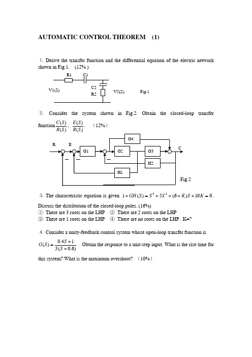
自动控制原理(中英文对照李道根)习题2题解
2C ov
� � R� R � ) s( iVs 1C � )s ( oV� s 1C � � � )s ( A V �� � 1� 1 � )c( � R R R �� � )s ( oV � )s ( A V� s 2 C � �� � 1 1 2 �� ) s ( iV
.5.2P erugiF
) s ( 2 X 2 s 2 M � ]) s ( 2 X � ) s ( 1 X [ K
snቤተ መጻሕፍቲ ባይዱituloS■
�
)s ( F )s( 2 X
3
3 Z 1Z � 3 Z 2 Z � 2 Z 1Z
3Z0 Z
��
)s ( iV )s ( oV
�
�3 2Z 2 1 �� � Z � Z � Z �� ) s ( oV � ) s( A V� � 1 1 1 �� � 1 � )d( 1 0Z� Z � � ) s ( iV � 1 1 � )s ( A V
2 3
�
) s( R )s ( C
evah ew ,yaw emas a nI )b( si noitcnuf refsnart eht ,ecneH
� ) s( R )s ( C
evah ew ,snoitidnoc laitini orez gnimussa ,mrofsnart ecalpaL gnikaT )a( :noituloS
C
)1 � s (s 0K
5X 2K 2N
4X
sT 1
3X
2X
1G
1X
1N
R
.nwohs sa margaid kcolb eht evah ew , redro ni thgir ot tfel morf )s ( C dna )s ( 5 X , ) s ( 4 X , ) s( 3 X , ) s ( 2 X , )s ( 1 X , )s (R selbairav eht gnignarraeR
L1自动控制原理

自动控制系统
3
控制理论的发展
原始控制设备
没有理论指导 单输入(SI) 多输入输出(MIMO)
经典控制理论
现代控制理论
大系统理论/复杂系统理论 智能控制理论
4
控制理论的发展
经典控制理论
研究的主要对象是单输入、单输出——单变量系统。 如:调节电压改变电机的速度;调整方向盘改变汽 车的运动轨迹等。
d m r(t) d m-1r(t) dr(t) bm b b b 0 r(t) m-1 1 m m-1 dt dt dt
式中:r(t)——系统输入量; c(t)——系统输出量 主要特点是具有叠加性和齐次性。
14
非线性系统
特点:在构成系统的环节中有一个或一个以上的非 线性环节。 非线性的理论研究远不如线性系统那么完整,目前 尚无通用的方法可以解决各类非线性系统。 近似处理。
放大器
执行机构 (步进电机)
工作机床
切削刀具
图纸
指令
8
自动控制系统的分类Leabharlann 闭环控制系统(反馈控制系统)
特点:系统输出信号与测量元件之间存在反馈回 路。 “闭环”这个术语的含义,就是将输出信号 通过测量元件反馈到系统的输入端,通过比较、 控制来减小系统误差。
微型计算机 放大器 执行机构 工作机床 切削刀具 位移
15
自动控制系统的分类
其他分类方式
按系统数学模型参数特性分:定常系统和时变系统 按功能分:温度控制系统、速度控制系统、位置控制 系统等。 按元件组成分:机电系统、液压系统、生物系统等。
自动控制原理(中英文对照 李道根)习题5题解
180
44
■Solutions
P5.5 Fig. P5.5 shows the polar plots of the open-loop transfer functions of some systems. Determine whether the closed-loop systems are stable. In each case, p is the number of the open-loop poles located in the right half s -plane, is the number of the integral factors in the open-loop transfer function.
( j )
4 9
2
2
2
2
, ( j ) arctan
4
arctan
9
40
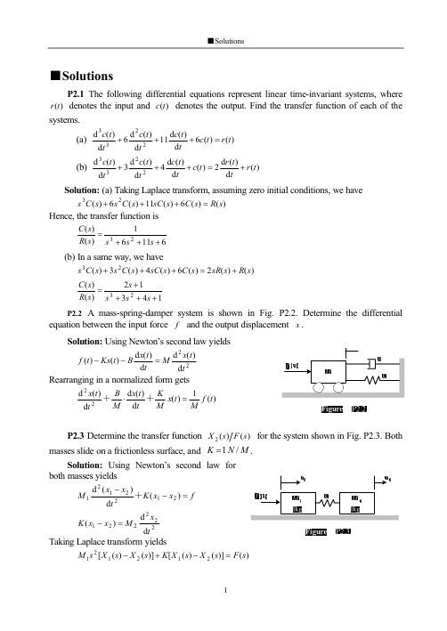
■Solutions
P5.3 Plot the asymptotic log-magnitude curves and phase curves for the following transfer functions (a) G ( s) H ( s) (c) G ( s) H ( s) (e) G ( s) H ( s)
(s )
G(s) 5 1 G (s ) 2s 6 5 (2 ) 6
2 2
( j )
, ( j ) arctan
2 6
respectively. (a) In the case of r (t ) sin(t 30 ) , since 1 and 0 30 , we have
《自动控制原理》部分中英文词汇对照表(英文解释)
《自动控制原理》部分中英文词汇对照表AAcceleration 加速度Angle of departure分离角Asymptotic stability渐近稳定性Automation自动化Auxiliary equation辅助方程BBacklash间隙Bandwidth带宽Block diagram方框图Bode diagram波特图CCauchy’s theorem高斯定理Characteristic equation特征方程Closed-loop control system闭环控制系统Constant常数Control system控制系统Controllability可控性Critical damping临界阻尼DDamping constant阻尼常数Damping ratio阻尼比DC control system直流控制系统Dead zone死区Delay time延迟时间Derivative control 微分控制Differential equations微分方程Digital computer compensator数字补偿器Dominant poles主导极点Dynamic equations动态方程EError coefficients误差系数Error transfer function误差传递函数FFeedback反馈Feedback compensation反馈补偿Feedback control systems反馈控制系统Feedback signal反馈信号Final-value theorem终值定理Frequency-domain analysis频域分析Frequency-domain design频域设计Friction摩擦GGain增益Generalized error coefficients广义误差系数IImpulse response脉冲响应Initial state初始状态Initial-value theorem初值定理Input vector输入向量Integral control积分控制Inverse z-transformation反Z变换JJordan block约当块Jordan canonical form约当标准形LLag-lead controller滞后-超前控制器Lag-lead network 滞后-超前网络Laplace transform拉氏变换Lead-lag controller超前-滞后控制器Linearization线性化Linear systems线性系统MMass质量Mathematical models数学模型Matrix矩阵Mechanical systems机械系统NNatural undamped frequency自然无阻尼频率Negative feedback负反馈Nichols chart尼科尔斯图Nonlinear control systems非线性控制系统Nyquist criterion柰奎斯特判据OObservability可观性Observer观测器Open-loop control system开环控制系统Output equations输出方程Output vector输出向量PParabolic input抛物线输入Partial fraction expansion部分分式展开PD controller比例微分控制器Peak time峰值时间Phase-lag controller相位滞后控制器Phase-lead controller相位超前控制器Phase margin相角裕度PID controller比例、积分微分控制器Polar plot极坐标图Poles definition极点定义Positive feedback正反馈Prefilter 前置滤波器Principle of the argument幅角原理RRamp error constant斜坡误差常数Ramp input斜坡输入Relative stability相对稳定性Resonant frequency共振频率Rise time上升时间调节时间 accommodation timeRobust system鲁棒系统Root loci根轨迹Routh tabulation(array)劳斯表SSampling frequency采样频率Sampling period采样周期Second-order system二阶系统Sensitivity灵敏度Series compensation串联补偿Settling time调节时间Signal flow graphs信号流图Similarity transformation相似变换Singularity奇点Spring弹簧Stability稳定性State diagram状态图State equations状态方程State feedback状态反馈State space状态空间State transition equation状态转移方程State transition matrix状态转移矩阵State variables状态变量State vector状态向量Steady-state error稳态误差Steady-state response稳态响应Step error constant阶跃误差常数Step input阶跃输入TTime delay时间延迟Time-domain analysis时域分析Time-domain design时域设计Time-invariant systems时不变系统Time-varying systems时变系统Type number型数Torque constant扭矩常数Transfer function转换方程Transient response暂态响应Transition matrix转移矩阵UUnit step response单位阶跃响应VVandermonde matrix范德蒙矩阵Velocity control system速度控制系统Velocity error constant速度误差常数ZZero-order hold零阶保持z-transfer function Z变换函数z-transform Z变换。
- 1、下载文档前请自行甄别文档内容的完整性,平台不提供额外的编辑、内容补充、找答案等附加服务。
- 2、"仅部分预览"的文档,不可在线预览部分如存在完整性等问题,可反馈申请退款(可完整预览的文档不适用该条件!)。
- 3、如文档侵犯您的权益,请联系客服反馈,我们会尽快为您处理(人工客服工作时间:9:00-18:30)。
《自动控制原理》课程教学大纲课程编号:2020161课程类别:必修授课对象:本科三年级先修课程:复变函数,积分变换,信号与系统。
学分:4总学时:56 课内学时:48 实验学时: 8一、课程性质、教学目的与任务课程性质:专业基础课,专业知识链条中的关键环节之一,自动控制原理是仪器仪表类、测控类专业的重要基础课之一,这些专业主要学习信号传感(获取)、信号处理、控制及光机电系统等知识,而控制是知识链条中的重要一环,随着科技发展,自动化、智能化已成为仪器、产品、系统等的重要功能,这就要求学生必须具备自动控制方面的知识。
教学目的与任务:培养学生自动控制原理的基础知识,学习掌握经典控制的基本理论、基本方法和控制系统的基本设计方法,重点学习分析和设计线性控制系统的基本理论、基本方法及控制系统设计方法。
主要内容包括:控制系统的数学模型、控制系统的时域分析法、控制系统的根轨迹法、控制系统的频域分析法、控制系统的常用校正方法等。
二、教学基本要求学习经典控制的基本理论和基本方法,重点学习分析和设计线性控制系统的基本理论和基本方法。
主要内容包括:控制系统的数学模型、控制系统的时域分析法、控制系统的根轨迹法、控制系统的频域分析法、控制系统的常用校正方法等。
三、教学内容第一章控制系统的一般要概念(4课时)自动控制的基本原理与方式,自动控制系统示例,自动控制系统的分类,对自动控制系统的基本要求1、基本概念;2、 反馈系统基本组成;3、 基本控制方式;4、 控制系统分类:开环、闭环、复合控制;第二章 控制系统的数学模型 (8课时)控制系统的时域数学模型,拉普拉斯变换,控制系统的复域数学模型,控制系统的状态空间模型,控制系统的结构图与信号流图2-1 时域模型、微分方程表示方法;2-2 复域模型1、 传递函数的定义与性质;2、 传递函数的零、极点表示,开环增益、根轨迹增益等;3、 典型环节的传递函数(比例、惯性、微分、积分、振荡);2-3 控制系统的结构图与信号流图1、 结构图的等效变换与化简2、 信号流图组成与性质A .性质、术语(理解)B .由结构图转化为信号流图方法C .梅逊公式第三章 线性系统的时域分析法 (10课时)线性系统时间响应的性能指标,一阶系统的时域分析,二阶系统的时域分析,高阶系统的时域分析,线性系统的稳定性分析,线性系统的稳态误差计算。
3-1 线性系统时间响应的性能标r t ,p t ,s t ,%σ3-2 一阶系统的单位阶跃响应,3-3 二阶系统的时域响应1、二阶系统的标准数学模型 闭环传递函数形式,表示为单位反馈系统形式2、二阶系统单位阶跃响应(重点:欠阻尼情形)r t ,p t ,s t ,%σ3、二阶系统性能改善A、比例一微分控制掌握原理、特点B、测速反馈控制掌握原理、特点及性能参数计算3-4高阶系统时域分析,主导闭环极点概念3-5线性系统稳定性分析劳斯判据及其应用3-6线性系统的稳态误差1、误差传递函数计算2、利用终值定理求稳态误差3、系统类型(型别)4、典型参考信号输入下的稳态误差;误差系数5、减小稳态误差方法:提高型别、提高开环增益、采用复合控制6、扰动误差的传函、减小扰动误差方法A、增加扰动作用点之前积分环节数目B、增加扰动作用点之前环节的增益C、采用复合控制技术第四章根轨迹(6课时)根轨迹方程,根轨迹绘制的基本法则,广义根轨迹,系统性能的分析与估算,基于根轨迹的控制系统校正方法,MATLAB语言根轨迹分析法。
4-1 根轨迹方程(相角、幅值条件)4-2 根轨迹绘制的基本法则,绘制根轨迹第五章线性系统的频域分析(10课时)频率特性,典型环节和开环系统频率特性,奈奎斯特稳定判据,稳定裕度,闭环频率特性,系统时域指标估算,传递函数的实验确定法,MATLAB语言频域分析法。
5-2 频率特性1、基本概念系统频率特性与传函间关系2、频率特性表示方法幅相曲线;幅频特性;对数幅频特性曲线;相频特性曲线;对数相频特性曲线5-3 典型环节和开环系统频率特性1、典型环节的幅频、相频特性2、开环对数幅频、幅相曲线绘制对数幅频特性采用渐近线法3、由幅频曲线或相频曲线确定最小相位系统传递函数的方法5-4 奈奎斯特稳定性判据1、奈代判据,实际使用判据,幅相曲线对称性2、对数频率特性稳定性判据 I型以上辅助线作法5-5稳定裕度概念:截止频率;相角交界频率;相角裕度;幅值裕度5-6闭环频率特性(了解)5-7系统时域指标与频域指标关系了解它们之间的联系;第六章线性系统的校正方法(10课时)系统的设计与校正问题,常用校正装置及其特性,串联校正,反馈校正,复合校正,PID调节器,基于MATLAB语言的校正分析法。
6-1 校正方法串联,反馈,前馈,复合,原理,特性6-2常用校正装置及其特性(传函,特性,重要公式)1、无源超前2、无源迟后3、无源迟后—超前6-3串联校正1、串联超前方法,实用范围2、串联迟后方法,实用范围3、串联迟后—超前方法,实用范围6-4反馈校正(原理,优点)6-5复合校正A.按扰动补偿(原理,扰动误差传函推导,误差全补偿条件)B.按输入补偿(原理,误差传函推导,误差全补偿条件)6-6 PID控制原理(P,PD,I,PI,PID的特点)实验安排:实验二直流电机速度控制实验(8课时)1、开环控制、闭环控制系统设计2、控制系统的校正设计3、PID调节器开放性、综合设计实验,要求学生独自完成实验前准备工作(实验目的、原理分析,实验设计、实验步骤、参数计算等),实际动手实验,实验结果分析等。
四、学时分配总学时 56学时讲课48学时实验8学时课外学时 64学时五、教材与参考资料胡寿松等,《自动控制原理》,国防工业出版社,第4版,2002[1] 自动控制原理,清华大学出版社,吴麒主编;[2] 自动控制原理,中国科学技术大学出版社,庞国仲编;[3] 自动控制原理试题精选与答题技巧,哈尔滨工业大学出版社,王彤主编;[4] 自动控制原理常见题型解析及模拟题,西北工业大学出版社,史忠科,卢京潮编著;[5] MATLAB 语言工具箱—TOOLBOX实用指南,西北工业大学出版社,施阳李俊等编著;[6] MATLAB 语言—演算纸式的科学工程计算语言,中国科学技术大学出版社,张培强主编;[7] 系统分析与仿真—MATLAB语言及应用,国防科技大学出版社,黄文梅杨勇等编著。
六、成绩评定期末成绩80%,平时成绩(作业、平时测验及课堂情况)及综合实验能力20%。
大纲撰写人:段发阶、吴斌大纲批准人:段发阶制定日期:2011年6月TJU Syllabus for “Automatic control principle”Code:Category: compulsoryFor: juniorPrerequisite:complex variables functions, integral transformation, Signals and SystemsCredits: 4Semester Hour: 56 Lecture: 48 Computer Lab:81.Course nature, teaching goal and missionCourse nature: As professional basic course, one of the key links of professional knowledge chain, automatic control theory is one of most important basic courses in majors of instruments and measure & control. These majors mainly study the knowledge of signal sensing (for), signal processing, control and optomechatronics system and so on, and control is an important link in the chain knowledge. Along with the development of science and technology, automation and intelligent have become important function in instrument, production, system, etc. This requires the students must have knowledge of automatic control aspects. Teaching goal and mission: Cultivate students the basic knowledge of automatic control principle. Learn to master the basic theory and basic method of classical control, and the basic design method of the control system. Learn mainly analysis and design of linear control system of basic theory, the basic method and control system design method. The main contents include: the mathematical model of control system, the time domain analysis method of the control system, the root locusmethod of the control system, the method of frequency domain of the control system, the commonly used correction methods of the control system, etc.2.Teaching basic requirementsThe basic requirements are learning the basic theories and methods of classical control, mainly learning the basic theory and basic methods of analysis and design of linear control system. The main contents include: the mathematical model of control system, the time domain analysis method of the control system, the root locus method of the control system, the frequency domain method of the control system, the commonly used correction methods of the control system, etc.3. Content of courses(4 hours)Chapter One, the general concepts of Control systemThe basic principle and means of automatic control, automatic control system examples, the classification of the automatic control system, the basic requirements of automatic control system1.Basic concept2.The basic structure of feedback system3.The basic control mode4. Control system classification: open loop, closed loop, composite control*Chapter Two, The mathematical model of the control system (8 hours) The mathematical model of time domain of the control system, Laplace transform, the complex domain mathematical model of the control system, the state space model of the control system, the structure and signal flow graph of the control system 2-1 The time domain model, differential equation expression method2-2 Complex domain model1.the definition and properties of the transfer function;2.zero and poles expression, the open loop gain, root locus gain, etc.of the transfer function3.the transfer function’s typical link (proportion, inertia,differential and integral, oscillation);2-3 The structure and signal flow diagram of the control system1. The equivalent transformation and simplification of the structurechart2. Signal flow chart composition and properties3. Properties, term (understand)a. The method of structure chart translate into signal flow graphb. Mason formulaChapter Three, time domain analysis method of the linear system (10 hours)The performance index of the linear system time response, analysisof time domain of the first-order system, analysis of time domain ofthe second-order systems, analysis of time domain of the high ordersystems, linear system stability analysis, the steady-state errorcalculation of linear system3-1 The performance standard of time response of the linear systemr t ,p t ,s t ,%σ3-2 The first-order system ’s unit step response ]3-3 Time domain response of the second order system1. The closed-loop transfer function form of the second order system ’s standard mathematical model, expresses as the form of unit feedbacksystem2. Unit step response of the second order system (Key: owe damping case)r t ,p t ,s t ,%σ3. System performance improved of the second order systemA. Proportion-differential control, master principle andcharacteristicsB. Velocity measurement feedback control, master the calculation ofprinciple, characteristics and performance parameter3-4 Analysis of time domain of the high order system, the concept of the leading close-loop poles3-5Linear system stability analysisLaws criterion and its application3-6 Steady-state error of linear system1.The calculation of error transfer functioning final-value theorem for steady-state error3.System type(pattern)4.The steady-state error of typical reference signal input; Errorcoefficient5.Reduce the steady-state error method: improve pattern, improve the openloop gain, and use composite control6. The transfer function of agitation error, the method of reduce agitation error(1). Increase integral element number before the agitationapplication point(2). Increase integral element gain before the agitationapplication pointAdopted complex control technologyChapter Four, Root locus (6 hours)Root locus equation, basic law of root locus rendering, generalized root locus, system performance analysis and estimate, the control system correction methods based on root trajectory, MATLAB language root locus analysis method.4-1 Root locus equation (Angle, amplitude condition)4-2 Basic law of root locus rendering, draw root locus*Chapter Five, frequency domain analysis of the linear systemFrequency characteristics, typical links and open loop system frequency characteristics, Nyquist stability criterion, the margin of the stable, closed-loop frequency characteristics, the system time domain indexes estimation, the experiment confirm method of the transfer function, the frequency domain method of MATLAB language5-2 Frequency characteristics1.The basic concept, the relationship between frequency characteristics andtransfer function of the system2.The expression method of frequency characteristics, phase curve; Amplitudefrequency characteristics; Logarithm amplitude frequency characteristics curve; Phase frequency characteristic curve; Logarithm phase frequency characteristic curve5-3Typical links and open loop system frequency characteristics1.Typical link’s amplitude frequency, phase frequency characteristics3.The open loop logarithm amplitude and frequency, amplitude and phase curvedrawing, logarithm amplitude frequency characteristics uses theasymptote method2.The minimum phase system transfer function method determined by amplitudefrequency curve or phase frequency curve5-4Nyquist stability criterion1.Nyquist criterion, actual use criterion, amplitude and phase curvesymmetry2.The stability criterion of log frequency characteristics auxiliary lineused in type I and above5-5 The concept of stability margin: cut-off frequency; Phase angle border frequency; the margin of the phase angle; amplitude margin5-6 Closed-loop frequency characteristics (know)5-7 the relationship between system time domain index and system frequency domain indexUnderstand the relationship between them*Chapter Six, Linear system calibration method (10 hours)The system design and correct problem, commonly used correction device and its characteristics, series correction, feedback correction, compound adjustment, PID regulator, the correction analysis method based on MATLAB language.6-1 Correction method series, feedback, feedforward, composite,principle, characteristics6-2 commonly used calibration device and its characteristics (transfer function, characteristics, important formula)1.Passive ahead2.Passive lag3.Passive lag-ahead6-3 Series correction1. Serial advanced method, practical scope2. Serial lag method, practical scope3. Serial lag-advanced method, practical scope6-4 Feedback correction (principle, advantages)6-5 Compound correctionA. According to the disturbance compensation (principle, the transferfunction derivation of disturbance error, error full compensationconditions)B. According to the input compensation (principle, the transferfunction derivation of error, error full compensation conditions) 6-6 PID control principle (the characteristics of P, PD, I, PI, PID) Experimental arrangement:Lab 2, DC motor speed control experiment (8 hours)1. Design of open loop control, closed loop control system2. Correction design of control system3. PID regulatorOpen, integrated design experiments, students are required to completethe preparation work alone before (experiment aim, principle analysis,experiment design, experiment steps, parameter calculation, etc.),practical experiments, the analysis of experimental results, etc.4. Semester Hour Structure5. Text-Book & Additional ReadingText-Book:“Automatic control principle”, Shousong Hu, etc. Defense industry press, version 4, 2002Additional Reading:[1] “Automatic control principle”, Qi Wu, etc. Qinghua Press[2] “Automatic control principle”, Guozhong Pang, etc. China scienceand technology university press[3] “Automatic control principle questions selected and examinationskills”, Tong Wang, etc. Harbin industrial university press[4] “Automatic control principle common question analytical andsimulation topic”, Zhongke Shi, Jingchao Lu, etc. northwestern university press[5] “MATLAB language TOOLBOX-TOOLBOX practical guide”, ShiYang northrop,etc. Northwestern university press[6] “MATLAB language-the operations paper type science and engineeringcalculation language”, PeiJiang Zhang, China science and technologyuniversity press;[7] “System analysis and simulation---MATLAB language and application”,WenMei Huang, Yong Yang, etc. National defense science and technology university press.6. GradingThe final examination 80%, Ordinary times (assignments, exams and class performance) and comprehensive experiment ability 20%.Data: 2011.6。