Poisson Image Editing
泊松融合matlab

泊松融合matlab
泊松融合是一种常用的图像处理算法,可以将两张不同的图片合并成一张完整的图片。
这种算法在数码相机、电影特效以及计算机视觉领域都有很广泛的应用。
在matlab中,实现泊松融合可以使用Image Processing Toolbox中的函数。
泊松融合的基本思路是将两张图像进行“剪切”和“粘贴”操作,即将一张图像中的某些区域剪切出来,然后将其粘贴到另一张图像中。
为了使得两张图像的边缘能够自然地衔接,需要使用泊松方程进行修正,从而达到更好的融合效果。
在matlab中,可以使用如下代码实现泊松融合:
```matlab
% 读入两张图像
A = imread('image1.jpg');
B = imread('image2.jpg');
% 获取A图像中需要剪切的区域
mask = roipoly(A);
% 对A图像中的剪切区域进行泊松融合
blended_image = poissonBlend(B, A, mask);
% 显示融合后的图像
imshow(blended_image);
```
上述代码中,通过调用roipoly函数获取图像A中需要剪切的区
域,然后使用poissonBlend函数进行泊松融合操作,最终得到融合后的图像。
需要注意的是,将两张图像进行泊松融合时,需要保证两张图像的大小和分辨率相同。
除了使用matlab自带的函数实现泊松融合之外,还可以使用第三方工具包,如OpenCV、Python等进行实现。
无论使用哪种工具包,都需要对泊松融合的算法原理有一定的了解,才能够更好地实现该算法。
Rectangling panoramic images via warping
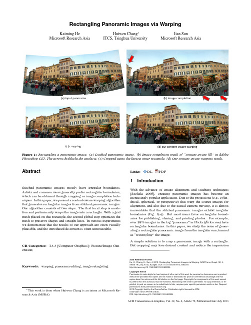
(b) image completion
(c) cropping
(d) our content-aware warping
Figure 1: Rectangling a panoramic image. (a) Stitched panoramic image. (b) Image completion result of “content-aware fill” in Adobe Photoshop CS5. The arrows highlight the artifacts. (c) Cropped using the largest inner rectangle. (d) Our content-aware warping result.
CR Categories: I.3.3 [Computer Graphics]: Picture/Image Generation;
Keywords: warping, panorama editing, image retargeting
ACM Reference Format He, K., Chang, H., Sun, J. 2013. Rectangling Panoramic Images via Warping. ACM Trans. Graph. 32, 4, Article 79 (July 2013), 9 pages. DOI = 10.1145/2461912.2462004 /10.1145/2461912.2462004. Copyright Notice Permission to make digital or hard copies of all or part of this work for personal or classroom use is granted without fee provided that copies are not made or distributed for profit or commercial advantage and that copies bear this notice and the full citation on the first page. Copyrights for components of this work owned by others than the author(s) must be honored. Abstracting with credit is permitted. To copy otherwise, or republish, to post on servers or to redistribute to lists, requires prior specific permission and/or a fee. Request permissions from permissions@. 2013 Copyright held by the Owner/Author. Publication rights licensed to ACM. 0730-0301/13/07-ART79 $15.00. DOI: /10.1145/2461912.2462004
泊松融合原理和python代码
泊松融合原理和python代码泊松融合(Poisson blending)是一种图像处理技术,用于将源图像中的对象融合到目标图像中,以实现无缝的图像合成。
该技术通过泊松方程求解,在图像融合中起到关键作用。
泊松融合的基本原理是通过将源图像中的像素值通过泊松方程融合到目标图像中,从而在目标图像中生成一个新的像素值,以实现图像融合的效果。
其数学表示如下:∇²α=∂²α/∂x²+∂²α/∂y²=β其中,α表示源图像中的像素值,β表示目标图像中的边缘像素值。
这个方程可以简化为拉普拉斯方程∆α=β,其中∆表示拉普拉斯算子。
这个方程的意义是,对于源图像中的像素α,其梯度的变化应该与目标图像中的边缘像素β相匹配。
根据泊松方程求解的目标,可以得到融合后的像素值。
在求解过程中,需要考虑边界条件和约束条件。
边界条件通常是指融合图像的边界像素值应与目标图像一致,约束条件通常是指源图像中的一些区域或者像素需要完全复制到目标图像中,从而实现融合效果。
下面是一个使用Python实现泊松融合的代码示例:```pythonimport numpy as npfrom scipy.sparse import linalgdef poisson_blend(source, target, mask):#获取图像的宽度和高度height, width, _ = target.shape#创建拉普拉斯矩阵A和边界像素矩阵bA = np.zeros((height * width, height * width))b = np.zeros(height * width)#根据源图像和目标图像计算拉普拉斯矩阵A和边界像素矩阵bfor y in range(1, height - 1):for x in range(1, width - 1):#当前像素在图像中的索引idx = y * width + xif mask[y, x] == 1:#如果是掩膜内的像素,使用泊松方程并加上约束条件A[idx, idx] = 4A[idx, idx - 1] = -1A[idx, idx + 1] = -1A[idx, idx - width] = -1A[idx, idx + width] = -1b[idx] = 4 * source[y, x] - source[y, x - 1] - source[y, x + 1] - source[y - 1, x] - source[y + 1, x]else:#如果是边界像素,直接复制到目标图像中A[idx, idx] = 1b[idx] = target[y, x]#使用稀疏矩阵求解线性方程组x = linalg.spsolve(A, b)# 将求解出的像素值reshape为目标图像的形状blend = x.reshape((height, width, 3)) return blend#加载源图像、目标图像和掩膜图像source = np.array(Image.open('source.jpg')) target = np.array(Image.open('target.jpg')) mask = np.array(Image.open('mask.png'))#对源图像和目标图像进行泊松融合blend = poisson_blend(source, target, mask) #显示融合后的图像plt.imshow(blend)plt.show```这段代码使用了`numpy`库和`scipy.sparse`库实现了泊松融合的算法。
泊松噪声模糊图像的边缘保持变分复原算法
u| ) d
( 3)
其中: 为图像的支持域; 约束函数 在图像梯度大的地方取 值较大, 在梯度小的地方取较小的值。通过求解式( 3) 的 Euler 方程, 可将其转化为非线性扩散方程, 即 u (| u | ) 2H (Hu - f ) = 0 ( 4) | u| 式中引入扩散系数 c( | u| ) = ( | u| )/ | u| 。一般来说, 扩散系数在图像的平坦区域取较大的值以抑制噪声, 而在图像 的边缘区域取较小的值以保护边缘。典型扩散系数的取值为 2 2 2 P -M 扩散方程, 其扩散系数为 c(x) = k / ( k + x ), k原方法
模型( 2) 采用光滑性先验时, 其复原结果对图像边缘的保 护较少, 使复原图像的边缘在某种程度上被平滑, 因而不能够 很好地保护图像的某些重要特征。基于非线性扩散的复原方 [ 9, 10] 法 , 考虑正则化变分模型, 即 J(u) = Hu - f
2 2
+
(|
( 1. School of Science, National University of Defense Technology , Changsha 410073, China; 2. Guilin Airforce Col lege, Guilin 541003, China)
Abstract: T he restoration of blurred image with Poisson noise was studied. According to the statistical maximum a posteriori MAP estimation of the original image, we built a new criterion to m easure the fidelity of the estimated image to the original image corrupted by Poisson noise. Because of the ill posed nature of the image restoration problem, we construct a new vari ational model with a regularization term. T he choice of the edge - preserving regularization function is addressed. To solve the variational m odel, we transform it to be a nonlinear diffusion equation. An adaptive regularization parameter, which can change its value from a smooth area to an edge area, is proposed. Numerical experiments demonstrate that the proposed method results in high restoration performance. T he new model can preserve edges and reduce the Poisson noise effectively. The improved signal to noise ratio( I SN R) is the new model is about 1 dB higher than the traditional iterative regularization method.
图像融合之泊松融合(PossionMatting)

图像融合之泊松融合(PossionMatting)前⾯有介绍拉普拉斯融合,今天说下OpenCV泊松融合使⽤。
顺便提⼀下,泊松是拉普拉斯的学⽣。
泊松融合的原理请参考这篇博⽂,讲的⾮常详细,此处不再赘述。
OpenCV中集成了泊松融合,API为seamless Clone(),函数原型如下: 泊松融合是将⼀个src放进dst中,放置位置根据dst中P点为中⼼的⼀个前景mask⼤⼩范围内。
融合过程会改变src图像中颜⾊以及梯度,达到⽆缝融合效果。
需要注意⼀点是,中⼼点P点的设置,最好是先根据前景mask算⼀个外接矩形框Rect,取Rect的中⼼点为P,保证Rect能够放进dst中,不会越界就好。
效果展⽰如下: src dstmask blend⽰例代码:1 #include <opencv2\opencv.hpp>2 #include <iostream>3 #include <string>45using namespace std;6using namespace cv;789void main()10 {11 Mat imgL = imread("data/apple.jpg");12 Mat imgR = imread("data/orange.jpg");1314int imgH = imgR.rows;15int imgW = imgR.cols;16 Mat mask = Mat::zeros(imgL.size(), CV_8UC1);17 mask(Rect(0,0, imgW*0.5, imgH)).setTo(255);18 cv::imshow("mask", mask);19 Point center(imgW*0.25, imgH*0.5);2021 Mat blendImg;22 seamlessClone(imgL, imgR, mask, center, blendImg, NORMAL_CLONE); 2324 cv::imshow("blendimg", blendImg);25 waitKey(0);26 }。
Simpleware ScanIP技术数据手册说明书

Import Formats• DICOM (version 3.0 and 2D stacks) including:–4D (time-resolved) DICOM with time step selection (in Simpleware ScanIP Medical only)–Option to store DICOM tags with imported data • DICOM encapsulated STL surface models (in Simpleware ScanIP Medical only)• ACR-NEMA (versions 1 and 2)• DICONDE • Interfile • Analyze • Meta-image • Raw image data • 2D image stacks: –BMP –GIF –JPEG –PCX –PNG –TIFF –XPM• Natively supported pixel types: –8-bit Unsigned Integer –16-bit Unsigned Integer –16-bit Signed Integer –32-bit Floating PointTECHNICAL DATASHEETExport Formats• Background 3D image: –RAW image –MetaImage–Stack of images (BMP , JPG, PNG, TIF) –DICOM• Background 4D image (in Simpleware ScanIP Medical only): –RAW image (all frames/active frame) –MetaImage (all frames/active frame) –Stack of images (active frame only) –DICOM (active frame only)• Segmented 3D image: –RAW image –MetaImage• Segmented 4D image (in Simpleware ScanIP Medical only): –Mask RAW (all frames/active frame) –Mask MetaImage (all frames/active frame)• Surface model (triangles): –STL –IGES –3MF –OBJ –PLY –ACIS (SAT) –ANSYS surfaceSimpleware ScanIP provides an extensive selection of image visualization, measurement and processing tools for working with 3D image data. Add-on modules are seamlessly combined to expand functionality.Simpleware ScanIPRelease Version U-2022.12Export Formats cont.• Surface model (triangles) cont.:–ABAQUS surface–OPEN INVENTOR–POINT CLOUD–MATLAB file surface–DICOM encapsulated STL (in SimplewareScanIP Medical only)• Animations:–AVI–Ogg Theora–H.264/MPEG-4 AVC–Windows Media Video (WMV)–PNG sequence–Transparent PNG sequence• 2D and 3D screenshot:–JPEG–PNG–Postscript (*.eps)–BMP–PNM–PDF• Generate virtual X-Ray, with object burn (in SimplewareScanIP Medical only)• Export scene – export the current 3D view:–3D PDF–3MF–OBJ–PLY–VRMLGeneral User Interface• Modern ribbon interface• Custom ribbon with user-selected tools (My tools)• Quick find search feature for tools• User-defined customization: dockable toolboxes, range of2D/3D view options• Undo/redo operation support• Independent part visibility control in 2D and 3D• Keyboard shortcuts: set user-defined shortcuts to commands or tools to customize and speed up repeated workflows• Ability to import multiple image sets into the workspace toaid segmentation• Histogram and profile line utilities assist in finding optimalthreshold values• Automatic logging and timestamp of filters and tools applied since the creation of a project• Workspace tabs: toggle between the active document, mask statistics, model statistics, centerline statistics, the document log, and the scripting interface• Integrated dynamic help tool• Interactive tutorials• Links to external support resources• Preferences: a number of different options available fordefault settings:–General: number of undos to save, default startup layout,max permissible CPUs for parallelized operations–Slice views: display orientation labels, choose whether touse a dark background, specify model contour and maskvoxel outline colors–PACS (in Simpleware ScanIP Medical only): two-way PACScommunication, configure access (servers, ports, keys etc.)–Segmentation: options to adjust behavior of somesegmentation tools and set Hounsfield presets forthe Threshold tool–3D view: save last camera position before exiting thedocument, stereo rendering settings, options to furtherdivide higher-order mesh elements (for FE meshesand NURBS patches)–Volume rendering: GPU rendering supported, Backgroundvolume rendering visibility on startup–Folders: options to change locations of temporary files–Statistics: default template for Mask, Model andCenterline statistics–Number formatting: customize how numbers are formatted within Simpleware ScanIP–Annotations: set default styles for annotations–Scripting: enable/disable supported scripting languages–Licensing: change license location–Miscellaneous: reset suppressible dialogs, clear the undo/redo stack, mask name/color creation options2D User Interface• 3x 2D views• Orientation labels• Scale bars• DICOM information overlay (in SimplewareScanIP Medical only)• Interactive cropping using 2D view• Window/Level values and control options• Ability to work on single slice, selection of slicesor whole volume• Slice cursors to identify the position of 2D slices2D User Interface cont.• Mask visualization options: solid, translucent, voxel outline • View 3D model contours from model/3D view, surface objects and volume meshes on 2D slices• Multi-planar reconstruction through translation and rotation of reslicing axes3D User Interface• Background volume rendering: using standard presets orgreyscale mapping• Single mask volume rendering• Interactive cropping using 3D view• Clipping box: unconstrained, interactive sectioningof 3D rendering• Fast 3D preview mode for rapid visualization of segmentation: ability to change preview quality to speed up rendering andreduce memory consumption• Live 3D: automatic 3D volume rendering refresh of masks • Mask transparency• Wireframe mode• Vertex lines superimposed over surfaces mode• Lighting and 3D rendering adjustments• Background adjustments:–Single color–Two color gradient–Skybox• View surface entities: CFD boundary conditions, node sets,contacts, shells• View contours of greyscale-based material properties• Model shading options: None, flat, Gouraud, hardware shader • Fullscreen mode• Camera control tool• Load and save 3D view camera positions• View slice planes• Slice intersection position widget• Show image dimensions on scale axes• 3D stereoscopic visualization with selected hardwaremodes available:–Crystal eyes–Red/blue–Interlaced–Left–Right–Dresden–Anaglyph–Checkerboard Image Processing Tools• Data processing:–Crop–Pad–Rescale–Shrink wrap–Resample using various interpolation techniques: nearestneighbor, linear, majority wins and partial volume effects–Flip–Shear–Align–Register datasets: Align background images to otherbackground images or any other dataset type based onsets of landmark points and/or automatic greyscale-based registration• Basic filters (most commonly used):–Smoothing: Recursive Gaussian, Smart masksmoothing, De-stepping–Noise filtering: mean filter, median filter–Cavity fill–Island removal filter–Fill gaps tool (using largest contact surface or mask priority)• Advanced filters (more specialist applications):–Binarization–Combine backgrounds–Connected component–Gradient magnitude–Lattice factory–Local maxima–MRI bias field correction (N4)–Masking filter–Morphological by reconstruction–Sigmoid–Simplify partial volume–Slice propagate–Distance maps:–Danielsson–Signed Maurer–CT correction:–CT image stabilizer–Histogram cylindrical equalization–Histogram slice equalization–Metal artefact reductionImage Processing Tools cont.• Advanced filters (more specialist applications) cont.:–Smoothing and noise removal:–Bilateral–Curvature anisotropic diffusion–Curvature flow–Discrete Gaussian–Gradient anisotropic diffusion–Min/max curvature flow–Patch-based denoising–Level sets:–Canny segmentation–Fast marching–Geodesic active contours–Laplacian level set–Shape detection–Threshold level set–Skeletonization:–Pruning–Thinning• Morphological filters:–Erode–Dilate–Open–Close–3D Wrap• Segmentation tools:–Paint/unpaint–Paint with threshold–Smart paint–Interpolation toolbox – Contains the following options:–Slice interpolation: smooth or linear–Slice propagation: adapts to image or uses direct copy–Confidence connect region growing–Background flood fill–Mask flood fill–Threshold–3D editing tools for application of filters to local regions –option to apply in multiple regions and on camera facingsurface only in advanced tool version–Mask ungroup tool–Automated generation of masks for pre- segmented images –Magnetic lasso–Multilevel Otsu segmentation–Split regions tool, with the ability to markregions in the 3D view–Merge regions tool–Direct copy: background to mask or mask to background–Watershed segmentation tool• Boolean operations: applied to/between masks. General and Venn diagram UI options:–Union–Intersect–Subtract–Invert• Local surface correction: local, greyscale-informed correction of mask surface, including the ability to apply on a regionof interest only• Multi-label tools: use mask labels to label different regionswithin a mask. Use for statistics and visualization:–Label disconnected regions–Split mask into pores–Combine masks to multi-label mask–Mask label editor–Reports (automatically generate pre-formatted reportsof common metrics using a multi-label mask orfull model’s mesh):–Particles report–Pores and throats report• Window/level tool• Overlap check: display/generate mask to check overlapvolume in active masksStatistical Analysis• Quick statistics: quickly compute commonly requiredquantities (volume, surface area, average greyscale, etc.)• Mask statistics (based on voxel information):–Built-in templates: general statistics, contact statistics,material statistics, orientation, pore sizes, surface statistics –Ability to generate user-defined templates–Variety of statistical information pertaining to:–Voxels: count, volume, surface area, etc.–Greyscales: mean, standard deviation,minimum, maximum, etc.–Surface estimation: area, area fraction, volume,volume fraction, etc.–Material properties: mass, mass density, Young’s modulus,Poisson’s ratio, moment of inertia, etc.–Axis-aligned bounding boxes–Axis-aligned bounding ellipsoidsStatistical Analysis cont.• Mask statistics (based on voxel information) cont.:–Object-oriented bounding boxes–Object-oriented bounding ellipsoids–Create a user-defined statistic• Model statistics (based on polygon information):–Ability to generate user-defined templates–Built-in templates: general statistics (perimeters, surfaces,volumes and NURBS surfaces), mesh quality (CFD, FE-linear elements and FE-quadratic elements), orientation(perimeters, surfaces, volumes), pore sizes, surface quality(linear, quadratic), volume mesh statistics–Variety of statistical information pertaining to:–Surface parameters: element count, node count,edge count, etc.–Perimeters: length, mean edge length, meandihedral angle, etc.–Surface triangle and quadrilateral primitives: edge- length,in-out ratio, distortion, etc.–Tetrahedral, hexahedral, pyramid and prismatic volumeelement primitives: angular skew, volume skew, shapefactor, Jacobian, etc.–Axis-aligned bounding boxes–Axis-aligned bounding ellipsoids–Object-oriented bounding boxes–Object-oriented bounding ellipsoids–Create a user-defined statistic• Centerline statistics:–Built-in templates: line orientation, lines by network, lines by node, constriction, shape, twist, nodes by network.–Ability to generate user-defined templates–Variety of statistical information pertaining to:–Lines: count, network, length, Euclidean length, curvature,torsion, closed, looped, positions, orientation, connectioncount, cross-sectional area and perimeter, incircle radius,twist, control points, object-oriented bounding boxes,mean orientation vector, best–fit circle, inscribed radius, circumscribed radius,bounding ellipse radius–Nodes: name, mask, network, position, line count,connection count.–Create a user-defined statistic–Probe centerlines to get measurements at specific locations • Save and import user-defined templates and statistics• Compute statistics within user-defined regions ofinterest (ROIs)Fiber Orientation Analysis• Allows fiber orientation to be analyzed directly from the image data (without the need for segmentation)• Option to include a mask representing the fiber region for fiber volume and diameter information• Specify the fiber diameter and the sampling size to beanalyzed for the whole image or a region of interest• Copy the centerlines generated during the analysis to thecenterlines editor for further editing or analysis• Statistics for analyzed region or region of interest:–Analyzed volume, fiber volume, fiber density,principal orientation–Eigen analysis (major, medial, minor vectors and value)–Orientation tensor–Fiber length and cross-section information• Plot statistics, export as *.png or *.csv:–Angle to principal orientation histogram–Angle to image axis histogram–Orientation tensor components vs image axis–Fiber density vs image axis (requires segmentation)–Principal orientation hedgehog diagram–Length of whole fibers histogram–Diameter of all segments histogram (incircle/best fit circle)(requires segmentation)• Visualize vectors:–Orientation vectors, Eigen vectors, Eigenellipsoids in 3D view–Orientation vectors in 2D slices–Change color scheme, and glyph density/scale/width–Export as *.csv or *.txt files• Map to mesh:–Export (or assign using FE Module) fiber orientationinformation per mesh cell–Average orientation tensor, eigenvector and eigenvalue data calculated for each mesh cell–Export volume fraction information per mesh cell(requires segmentation)Particle Analysis• Allows particles (either isolated or touching) to be analyzed from a mask or multi-label mask• There are two types of pore analysis available, “Touching”,for particles that are in contact with each other, “Isolated” for particles that are separated from each other.• Statistics for analyzed region or region of interest:–Particle volume (Total, Mean, SD, Min, Max)–Particle area (Mean, SD, Min, Max)–Particle volume fraction–Particle equivalent volume sphere diameter(Mean, SD, Min, Max)–Particle bounding box extent (Mean, SD, Min, Max)–Particle ellipsoid diameter (Mean, SD, Min, Max)–Particle flatness–Particle elongation–Particle shape factor–Particle sphericity• Plot statistics, export as *.png or *.csv:–Volume histogram–Area histogram–Flatness histogram–Elongation histogram–Shape factor histogram–Sphericity histogram• Particle visualization:–Contact count–Voxel count–Surface area–Boundary contact area–Label contact area–Volume–Max greyscale–Mean greyscale–Major length–Flatness–Elongation–Shape factor–Sphericity–Orientation angle to x/y/z axis–Orientation to mean–Export as *.csv or *.txt files• Map to mesh:–Export (or assign using FE Module) particle volume fraction information per mesh cell Pore Analysis• Allows pores (either open or closed) to be analyzed from a mask or multi-label mask• There are two types of pore analysis available, “Open”, for connected pore networks, and “Closed” for pores that are separated from each other• Statistics for analyzed region or region of interest:–Total pores count–Total throat count volume–Volume fraction–Internal pore volume (Mean, SD, Min, Max)–Internal pore surface area (Mean, SD, Min, Max)–Pore equivalent volume sphere diameter(Mean, SD, Min, Max)–Pore Flatness (Mean, SD, Min, Max)• Statistics for analyzed region or region of interest cont.–Pore Elongation (Mean, SD, Min, Max)–Pore Shape factor (Mean, SD, Min, Max)–Pore Sphericity (Mean, SD, Min, Max)–Pore coordination number (Mean, SD, Min, Max)–Throat contact count–Throat contact area–Throat radius (Mean, SD, Min, Max)–Throat Flatness (Mean, SD, Min, Max)–Throat Elongation (Mean, SD, Min, Max)–Throat Eccentricity (Mean, SD, Min, Max)–Throat Shape factor (Mean, SD, Min, Max)• Plot statistics, export as *.png or *.csv:–Volume histogram–Area histogram–Flatness histogram–Elongation histogram–Shape factor histogram–Sphericity histogram• Particle visualization:–Contact count–Voxel count–Surface area–Boundary contact area–Label contact area–Volume–Max greyscale–Mean greyscale–Major lengthPore Analysis cont.• Particle visualization cont.:–Flatness–Elongation–Shape factor–Sphericity–Orientation angle to x/y/z axis–Orientation to mean–Export as *.csv or *.txt files• Map to mesh:–Export (or assign using FE Module) pore volume fractioninformation per mesh cellSurface Mesh Generation• Topology and volume preserving smoothing• Triangle smoothing• Decimation• Multipart surface creation• Surface element quality control (for volume meshing in third party software)• So-called ‘sub-pixel accuracy’ through the use of partialvolume effects dataSurface Mesh Quality Inspection Tool• Inspect surface triangles or clusters of triangles• Option to show mesh errors (e.g. surface holes, surfaceintersections) and warnings• Show distorted elements above a user-defined threshold • Display quality metric histograms• Zoom into the pathological element to inspect it more closely Measurement Tools• Create and save points, distances and angles in 2D/3D• Visualization options to display all at once or selected• Snap to 3D surface option• Profile line• Histogram• Export as comma-separated values• Centerline creation toolkit:–Centerline creation (general)–Centerline creation for fibers–Junction editing• 2D contour measurements:–Creation mode–Area–Total perimeter–In-circle diameter–Out-circle diameter–Trigone-Trigone (TT) distance–Septal to Lateral (SL) distance–Intercommissural (IC) distance–Posterior perimeter• Wall thickness analysis tool for masks or surface objects,using a raycasting or sphere fitting algorithm• Shape-based measurement tools:–Shape editor: Create, edit, visualize, exportand measure shapes–Shape fitting: Fit shapes to geometry–Shape-to-shape measurements: Obtain measurementsbetween shape objects• X-ray image import, with alignment and object registration (in Simpleware ScanIP Medical only)3D Printing Toolkit• Set of tools for editing, analyzing and visualizing surfacesbefore sending them to a 3D printer which includes:–Preparation tools:–Model preview–Mask to Surface–Emboss text–Hollow–Cut–Create Connectors (inc. manual and automatic options)–Pins and Sockets connectors–Analysis tool – Greyscale visualization–Inspection tools:–Color proofing–Check printability–E xport: a variety of file formats including:–3MF–STL–OBJ–PLY–3D PDF–VRML©2022 Synopsys, Inc. All rights reserved. Synopsys is a trademark of Synopsys, Inc. in the United States and other countries. A list of Synopsys trademarks is available at /copyright.html . All other names mentioned herein are trademarks or registered trademarks of their respective owners.Animations• Create and export animations in the 3D view • Built-in-quick animations: –Rotations –Slice reveals –Volume rendering• User-defined animations cues: –Background colors–Camera (orbits, follow path and key frame-based), –Clipping –Opacity –2D slice planes –Volume rendering • Export formats: –AVI –Ogg Theora –H.264/MPEG-4 AVC–Windows Media Video (WMV) –PNG sequence• Variety of export sizes: From 480p to 2160p (4K)4D Frame Toolbox (in Simpleware ScanIP Medical only)• Active frame slider to manually control frame displayed in the 2D slice views and 3D view• Cine mode for active slice view and 3D view • Compare frames – compare two 2D slice views to examine differences• Options to set the time between frames and delete unwanted framesScripting• The ScanIP Application Programming Interface (API) is an object-oriented programming library that allows access to most of the features of Simpleware ScanIP • Support for a variety of scripting languages: –Python 3 –C#–Python 2 (deprecated) –Iron python (deprecated) –Visual basic (deprecated) –Boo (deprecated) –Java (deprecated)• Macro recording: record, save and play macro • Convert log entry to script• Script editor with autocomplete functionality• Console ScanIP: a GUI-less version of Simpleware ScanIP which can be run with scripted workflows。
EmguCV类(CvInvoke_Class) 方法整理

为数组的特定元素分配新值
Determinant
返回方阵矩阵的行列式。
Eigen
计算对称矩阵的特征值和特征向量
Exp
计算输入数组的每个元素的指数
dst(I)= exp(src(I))
FindFundamentalMat
使用四种方法之一计算基本矩阵,如果没有找到矩阵,则返回找到的基本矩阵(1或3)和0的数量
计算源数据的加权平均和,使得acc变为帧序列的运行平均值(Calculates weighted sum of input src and the accumulator acc so that acc becomes a running average of frame sequence: acc(x,y)=(1-alpha) * acc(x,y) + alpha * image(x,y) if mask(x,y)!=0 where alpha regulates update speed (how fastaccumulator forgets about previous frames).
SolvePnPRansac
利用Ransac方法利用点对求解相机姿态
StereoRectify
计算每个摄像机的旋转矩阵(虚拟地)使两个摄像机图像平面处于相同的平面。
Undistort
转换图像以补偿径向和切向透镜失真
UndistortPoints
与cvInitUndistortRectifyMap相似但也不同,相似的内容是他们都可用于校正镜头失真和透视变换。不同的是函数cvInitUndistortRectifyMap实际上执行的是反向转换以初始化地图,而这个函数执行的是正向变换。
泊松融合原理和python代码

泊松融合原理与Python代码实现1. 前言泊松融合是一种图像处理技术,用于将源图像的内容无缝地融合到目标图像中。
它的基本原理是通过解决一个泊松方程,将源图像的梯度与目标图像的梯度相匹配,从而实现融合效果。
在本文中,我们将详细介绍泊松融合的基本原理,并使用Python编写代码来实现泊松融合。
2. 泊松方程首先,让我们来了解一下泊松方程。
泊松方程是一个偏微分方程,通常用于描述物理系统中的平衡状态。
在图像处理中,我们可以使用泊松方程来实现无缝融合。
泊松方程可以表示为:∇²f = g其中,∇²表示拉普拉斯算子(二阶导数),f表示未知函数,g表示已知函数。
在泊松融合中,我们希望通过求解这个方程来得到未知函数f。
3. 泊松融合原理泊松融合的基本原理是将源图像的梯度与目标图像的梯度相匹配。
通过匹配这些梯度,我们可以确保融合后的图像在边界处具有连续性。
具体来说,泊松融合的步骤如下:1.将源图像和目标图像进行对齐。
对齐可以使用特征点匹配或其他图像对齐算法来实现。
2.在目标图像上选择一个感兴趣区域(ROI),并在该区域内将源图像的内容融合进去。
3.计算源图像和目标图像的梯度。
我们可以使用Sobel算子等滤波器来计算梯度。
4.在ROI中,将泊松方程应用于目标图像的梯度和源图像的梯度之间的差异。
这相当于求解泊松方程中的未知函数f。
5.将求解得到的未知函数f与目标图像中ROI外的部分进行融合,得到最终的融合结果。
4. Python代码实现接下来,让我们使用Python编写代码来实现泊松融合。
首先,我们需要导入所需的库:import numpy as npimport cv2from scipy import sparsefrom scipy.sparse.linalg import spsolve然后,我们定义一个名为poisson_blend的函数来执行泊松融合:def poisson_blend(source, target, mask):# 获取源图像和目标图像的尺寸height, width, _ = source.shape# 将源图像和目标图像转换为灰度图像source_gray = cv2.cvtColor(source, cv2.COLOR_BGR2GRAY)target_gray = cv2.cvtColor(target, cv2.COLOR_BGR2GRAY)# 计算源图像和目标图像的梯度source_grad_x = cv2.Sobel(source_gray, cv2.CV_64F, 1, 0, ksize=3)source_grad_y = cv2.Sobel(source_gray, cv2.CV_64F, 0, 1, ksize=3)target_grad_x = cv2.Sobel(target_gray, cv2.CV_64F, 1, 0, ksize=3)target_grad_y = cv2.Sobel(target_gray, cv2.CV_64F, 0, 1, ksize=3)# 创建稀疏矩阵A和向量bA = sparse.lil_matrix((height * width, height * width))b = np.zeros((height * width,))# 填充矩阵A和向量bfor y in range(1,height-1):for x in range(1,width-1):if mask[y,x] == 255:index = y * width + xA[index,index] = -4A[index,index-1] = 1A[index,index+1] = 1A[index,index-width] = 1A[index,index+width] = 1b[index] = target_grad_x[y,x] - target_grad_x[y,x-1] + target_ grad_y[y,x] - target_grad_y[y-1,x]# 解泊松方程f = spsolve(A.tocsr(), b)# 将求解得到的未知函数f转换为图像f_image = np.uint8(np.clip(f.reshape(height, width), 0, 255))# 在目标图像中将ROI外的部分与源图像进行融合blended = target.copy()for y in range(height):for x in range(width):if mask[y,x] == 255:blended[y,x] = source[y,x]return blended最后,我们加载源图像、目标图像和蒙版,并调用poisson_blend函数来执行泊松融合:source = cv2.imread('source.jpg')target = cv2.imread('target.jpg')mask = cv2.imread('mask.jpg', cv2.IMREAD_GRAYSCALE)result = poisson_blend(source, target, mask)cv2.imwrite('result.jpg', result)5. 总结在本文中,我们详细介绍了泊松融合的基本原理,并使用Python编写了相应的代码实现。
- 1、下载文档前请自行甄别文档内容的完整性,平台不提供额外的编辑、内容补充、找答案等附加服务。
- 2、"仅部分预览"的文档,不可在线预览部分如存在完整性等问题,可反馈申请退款(可完整预览的文档不适用该条件!)。
- 3、如文档侵犯您的权益,请联系客服反馈,我们会尽快为您处理(人工客服工作时间:9:00-18:30)。
Ω
〈 p,q〉∩Ω≠0
p+q w here vpq is the projection of v( ) on the oriented edge [ p, q] 2 p +q i.e., vpq = v( ) ⋅ pq 2 Its solution satisfies the following simultaneous linear equation:
Guided Interpolation
A guided field is a vector field v used in an extended version of minimization problem (1):
m ∫∫ ∇f − v in
f Ω
2
with f
= f* ∂Ω
∂Ω
(3)
This solution is the unique solution of following Poisson equation with Dirichlet boundary condition:
It computes the function whose gradient is the closet to some prescribed vector field-the guidance vector field-under given boundary conditions
Partial differential equation (PDE)
∂Ω
∂2. ∂2. w ere ∆. = 2 + 2 is th laplacian operator h e ∂x ∂y
(2)
Guided Interpolation
Equation 2 is a Laplace equation with Dirichlet boundary conditions.
Introduction
The Poisson equation has been used extensively in computer vision. The mathematical tool at the heart of this approach is the Poisson partial differential equation with Dirichlet boundary conditions which specifies the Laplacian of an unknown function over the domain of interest, along with the unknown function values over the boundary of domain. Solving the Poisson equation also has an alternative interpretation as a minimization problem:
i.e., 0.4s. per system on a Pentium 4 for a disk-shaped region of 60,000 pixels.
Seamless cloning
Importing gradients The basic choice for the guidance field v is a gradient field taken directly from a source image. Denoting by g this source image, the interpolation is performed under the guidance of
Importing gradients
Importing gradients
Seamless cloning
Mixing gradients
There are situations where it is desirable to combine properties of f* with those of g, for example to add objects with holes ,or partially transparent ones, on top of a textured or cluttered background. An example is shown in Fig.6
Guided Interpolation
The simplest interpolant f of f* over Ω is the membrane interpolant defined as the solution of the minimization 2 problem: *
m ∫∫ ∇f in
T = f (t) , at x = 0 , t > 0
T0
T = T1 ,
t>0
T= T , 1
T = T0 ,
at x =1, t > 0
at x > 0 , t = 0
0
1
x
圖 平版Dirichlet Condition 示意圖
Neumann condition
Neumann condition係指依變數之變化率之邊 界條件為定值,抑或獨立變數之函數之情況。 例如 ∂T = f (t) , at t = 0 , 0 ≤ x ≤1 或 ∂x ∂T = 0 , at x = 1, t ≥0 Neumann型邊界條件,亦稱為natural ∂x boundary condition。
Discrete Poisson solver
The finite difference discretization of (3) yields the following discrete, quadratic optimization problem: * m in ∑( f p − fq −vpq )2, w f p = f p , for all p∈∂Ω ith (6)
Poisson Image Editing
Patrick Perez Michel Gangnet Andrew Blake Microsoft Research UK
Outline
Introduction Poisson solution to guided interpolation
Guided Interpolation Discrete Poisson solver
方程式類別 橢圓型 拋物線型 雙曲線型 判斷式
b − 4ac < 0
2
代表性範例 Laplace方程式 Poisson方程式 波動方程式
∂2u ∂2u + 2 =0 2 ∂x ∂y
b2 − 4ac = 0
b − 4ac > 0
2
∂2u ∂2u + 2 = f (x, y) 2 ∂x ∂y
∂2u ∂2u = 2 α 2 ∂x ∂t
Seamless cloning
Importing gradients Mixing gradients
Selection editing
Texture flattening Local illumination change Local color change Seamless tiling
Conclusion
for all p∈Ω, Np f p −
q q∈Np ∩Ω
∑f
=
q* q∈Np ∩∂Ω
∑f
+ ∑vpq
q∈Np
(7)
Discrete Poisson solver
Equation (7) form a classical, sparse (banded), symmetric, positive-definite system. Results shown in this paper have been computed using either Gauss-Seidel iteration with successive overrelaxation or V-cycle multigrid. Both methods are fast enough
2
起始條件和邊界條件的分類
為了能獲得偏微分方程式之解答,其起始條 件和邊界條件可依其特性區分為三類。
第一類:Dirichlet Condition Dirichlet 第二類:Neumann condition 第三類:Robbins condition
Dirichlet Condiction
若依變數(T)本身,在某個獨立變數值時, 被指定,則此條件稱為Dirichlet Condition,亦稱為essential邊界條件。 下圖為一典型的Dirichlet條件示意圖 由圖中很清楚的顯示,該平板之邊界條 = f (t ), T 件為 t >0
for all 〈 p, q〉, vpq = gp − gq
(11)
Importing gradients
The seamless cloning tool thus obtained ensures the compliance of source and destination boundaries. It can be used to conceal undesirable image features or to insert new elements in an image, but with much more flexibility
∂u ∂v + is the divergence of v = (u, v) ∂x ∂y
Discrete Poisson solver
S Ωnow become finite point sets defined on an infinite discrete grid. Note that S can include all the pixels of an image or only a subset of them. For each pixel p in S, let Np be the set of its 4connected neighbors which are in S, and let <p,q> denote a pixel pair such that q∈Np The boundary of Ω is now ∂Ω ={p∈S \ Ω: Np ∩Ω ≠ 0} Let fp be the value of f at p and f Ω ={ f p , p∈Ω }