cellSens用户手册
TISON细胞系编辑器用户手册说明书

This page has been intentionally left blankLibrary Section (5)Canvas Toolbar (Left) (5)5.1.3 Create Cell Line (5)5.1.4 Account (6)5.1.5 Editor Logo (6)5.1.6 Canvas Toolbar (Bottom) (6)5.1.7 Project Panel (7)‘Create Cell Line’ Button (8)‘Show Cell Lines Library’ button (13)‘Upload Case Study’ Button (15)‘Import Cell Line’ Button (16)‘Report a Bug’ Button (18)‘Help’ Button (19)‘Edit Properties’ Button (21)‘Export Cell Line’ Button (22)‘Delete’ Button (24)Table of FiguresFigure 5.1.1 - The GUI of TISON’s CLE (4)Figure 5.2.1.1 - ‘Create cell line’ options in CLE... (8)Figure 5.2.1.2 - ‘Cell Line Properties’ window (9)Figure 5.2.1.3 - CLE GUI after the creation of a new cell line (10)Figure 5.2.1.4 - Error prompt display (10)Figure 5.2.1.5 - Error prompt display (11)Figure 5.2.1.6 - Error prompt display (11)Figure 5.2.1.7 - Selecting a saved cell line displays editing options (12)Figure 5.2.2.1 - ‘Show Cell Lines’ button in CLE (13)Figure 5.2.2.2 - Predefined cell circuits can be viewed in the library panel (14)Figure 5.2.3.1 - ‘Upload Case Study’ button in CLE... .. (15)Figure 5.2.3.2 - ‘Upload Case Study’ window in CLE (16)Figure 5.2.4. 1 - ‘Import cell line’ button in CLE (16)Figure 5.2.4. 2 - Import cell line window where user can select the (.txt) file for import (17)Figure 5.2.4.3 - A sample (portion) file (.txt) from the ‘Export Cell Line’ feature of CLE (18)Figure 5.2.5.1 - ‘Report a bug’ button in CLE..... (19)Figure 5.2.5.2 - GitHub page for reporting TISON’s bugs. (19)Figure 5.2.6.1 - ‘Help’ button in CLE... (20)Figure 5.2.7.1 - ‘Edit Properties’ button in CLE. (21)Figure 5.2.7.2 - ‘Edit Cell Line Properties’ window (22)Figure 5.2.8.1 - ‘Export Cell Line’ button in CLE.... (23)Figure 5.2.9.1 - ‘Delete’ button in CLE (24)Figure 5.2.9.2 - Confirmation prompt on selecting the delete option (24)List of TablesTable 5.2.1 - Video Tutorial for CLE (25)5. Cell Lines EditorCell Lines Editor (CLE) allows the user to create in-silico cell lines by assigning a particular cell circuit constructed using Cell Circuit Editor (CCE). Specifically, CLE allows the user to associate the cell line phenotype with the corresponding networks, therapies, and environments embedded within the assigned cell circuit. The graphical user interface (GUI), analysis techniques, and results visualization in the CLE are detailed ahead.CLE provides an intuitive GUI to access the underlying functionalities and features of the editor shown in Figure 5.1.1. Various sections and toolbars of CLE’s intuitive GUI have been labeled, and each feature’s functionality has been explained below.Graphical User InterfaceIn Figure 5.1.1,various sections and toolbars of Cell Lines Editor’s intuitive GUI have been labeled, and the functionality of each feature has been explained below.Figure 5.1.1 - The GUI of TISON’s CLE.Library SectionIn Figure 5.1.1 (A),∙The left panel provides access to the library of user-designed and saved cell lines. The user can ‘Edit Properties’, ‘Duplicate’, and ‘Delete’ constructed cell lines.∙Th e ‘Cell Lines’ panel (Figure 5.2.2.1) displays the saved cell lines created using CLE.∙The ‘Cell Circuits’ panel (Figure 5.2.2.2) displays the cell circuits constructed in the Cell Circuits Editor (CCE).Canvas Toolbar (Left)In Figure 5.1.1 (B),∙‘Create Cell Line’ button in the toolbar creates a new cell line.∙‘Show Cell Lines Library’ button displays and hides the library section.∙‘Upload Case Study’ button allows the user to upload template cell lines from the database.∙‘Import Cell Line’ button allows the user to upload a cell line from a cell line parameters file.∙‘Report a Bug’ button opens https:///BIRL/TISON/issues and allows the user to report any bug/issue in TISON.∙‘Help’ button opens the ‘Cell Lines Editor Manual’located on https://.pk/Manuals/CellLinesManual.pdf5.1.3 Create Cell LineIn Figure 5.1.1 (C),∙The text at the top left corner of the canvas displays the number of cell lines created using CLE, and the total number of networks, therapies, environments, and cell circuits used.∙The ‘C reate Cell Line’ box allows the user to create a cell line and opens a window to assign a cell circuit to the current cell line.5.1.4 AccountIn Figure 5.1.1 (D),∙Text at the top right corner of the canvas displays the username saved during the registration process.∙‘Return to Project Explorer’ icon in the account settings panel takes the user back to the project explorer and shows a list of all the projects.∙User icon allows the user to either return to TISON’s home page via ‘Main’ or sign out from TISON via ‘Sign Out’.5.1.5 Editor Logo∙In Figure 5.1.1 (E), the editor logo and text at the bottom right corner of the canvas display the editor being used.5.1.6 Canvas Toolbar (Bottom)∙In Figure 5.1.1 (F), the toolbar at the bottom of the canvas allows the user to switch between different editors in TISON.works button navigates to “Networks Editor.”2.Therapeutics button navigates to “Therapeutics Editor.”3.Environments button navigates to “Environments Editor.”4.Cell Circuits button navigates to “Cell Circuits Editor.”5.Cell Lines button navigates to “Cell Lines Editor.”6. Organoids button navigates to “Organoids Editor.”7.Simulations button navigates to “Simulations Editor.”8.Analytics button navigates to “Analytics Editor.”5.1.7 Project PanelIn Figure 5.1.1 (G),∙‘TISON Home’ button on the bottom left corner of the canvas takes the user back to TISON’s home page.∙‘Project Information’ button displays the project name at the bottom left corner of the canvas and takes the user back to the ‘Project Explorer’ page.Features ListA guide to the functionality of each GUI button and the parameters required by the user to build an in-silico cell line is provided in the following sections.‘Create Cell Line’ ButtonThe ‘Create Cell Line’ button in the left canvas toolbar (highlighted in Figure 5.2.1.1) allows the user to create a new cell line; the user can also create a cell line using the ‘Create Cell Line’ box.Figure 5.2.1.1 -‘Create cell line’ options in CLE.Clicking on the ‘Create Cell Line’ button or box opens the‘Cell Line Properties’ window shown in (Figure 5.2.1.2). This modal allows the user to enter the name, assign the validated cell circuit from the database, upload an image, and give a description for the new cell line.Figure 5.2.1.2 - ‘Cell Line Properties’ window.After providing all the necessary details, clicking on ‘Save’ will build the user-defined in-silico cell line, as shown in( Figure 5.2.1.3)Figure 5.2.1.3 - CLE GUI after the creation of a new cell line.If the user does not provide the name for the cell line they have designed, the following error prompt will appear on the canvas (Figure 5.2.1.4).Figure 5.2.1.4 - Error prompt display.Note that one cell circuit can only be assigned to one cell line; the following error prompt will appear on the canvas if the user selects a previously assigned cell circuit to a new cell line (Figure 5.2.1.5 - Error prompt display.).Figure 5.2.1.5 - Error prompt display.Moreover, each cell line must be assigned a unique name; repeating a name will prompt the following error message to appear (Figure 5.2.1.6 - Error prompt display).Figure 5.2.1.6 - Error prompt displayThe library panel allows the user to view the saved cell lines in the database. Any of the user’s pre-constructed cell lines can be loaded from the library section by double-clicking on their respective names. The selected cell line gets highlighted in grey to help the user locate the cell line in use; moreover, the user can also ‘Edit Properties’,‘Duplicate’, and ‘Delete’ a cell line by clicking the icons displayed in (Figure 5.2.1.5).Figure 5.2.1.5 - Selecting a saved cell line displays editing options: (a) Button for editing cell line properties (b) Button for duplicating the cell line (c) Button for deleting the cell line.‘Show Cell Lines Library’ button‘Show cell lines library’ button (Figure 5.2.2.1Figure 5.2.2.1 ) has a toggling action that provides the option to display or hide the library panel (i.e., if the library is open, it will close it and vice versa).Figure 5.2.2.1 - ‘Show Cell Lines’ button in CLE.The user can also view predefined cell circuits designed using CCE from the library panel, as shown below (Figure 5.2.2.2).Figure 5.2.2.2 - Predefined cell circuits can be viewed in the library panel.‘Upload Case Study’ Button‘Upload Case Study’ button (Figure 5.2.3.1) allows the user to open the provided case studies.Figure 5.2.3.1 - ‘Upload Case Study’ button in CLE.Predefined case studies have been incorporated into TISON’s CLE to guide the user toward s designing in-silico cell line models. Once the user clicks on the ‘Upload Case Study’ button, the window shown in Figure 5.2.3.2 appears, displaying a list of predefined case studies in CLE. Currently, CLE supports one pre-defined case study: (i) Case Study 1 – p53 network with DNA damage ON and OFF and (ii) Case Study2 – p53 network DNA with damage OFF integrated with environment (For visual reference, see section TISON’s Cell Lines Video Tutorial, Table 5.2.1 - Video 1).Figure 5.2.3.2 - ‘Upload Case Study’ window in CLE.‘Import Cell Line’ Button‘Import Cell Line’ button (highlighted in Figure 5.2.4.1 - ‘Import cell line’ button in CLE.) allows the user to upload an in-silico cell line file.Figure 5.2.4.1 - ‘Import cell line’ button in CLE.When the user selects the ‘I mport Cell Line’ button, the following model appears (Figure 5.2.4.1 - ‘Import cell line’ button in CLE Figure 5.2.4.2)Figure 5.2.4.2 - Import cell line window where user can select the (.txt) file for import.A sample cell line file that can be imported through this feature. Such a cell line file can be downloaded for any saved cell line in the CLE from the ‘Export Cell Line’ button mentioned in the following Figure 5.2.4.3 - A sample (portion) file (.txt) from the ‘Export Cell Line’ feature of CLE. The same file can be used for the ‘Import Cell Line’ feature..Figure 5.2.4.3 - A sample (portion) file (.txt) from the ‘Export Cell Line’ feature of CLE.The same file can beused for the ‘Import Cell Line’ feature.‘Report a Bug’ ButtonUpon encountering any problem in the software, the user can report the bug by clicking on the ‘Report a Bug’ button highlighted in Figure 5.2.5.1.Figure 5.2.5.1 - ‘Report a bug’ button in CLE.This button directs the user to a page on GitHub (Issues - BIRL/TISON - GitHub), where the user can report their issue (Figure 5.2.5.2).Figure 5.2.5.2 - GitHub page for reporting TISON’s bugs.‘Help’ ButtonSelecting the ‘Help’ button highlighted in Figure 5.2.6.1 opens a user guide manual of the editor currently in use (https://.pk/Manuals/CellLinesManual.pdf).Figure 5.2.6.1 - ‘Help’ button in CLE.‘Edit Properties’ ButtonUpon clicking the ‘Edit Properties’ button highlighted in Figure 5.2.7.1, the ‘Edit Cell Line Properties’ window, shown in Figure 5.2.7.2, appears. The user can change the cell line name, re-assign a cell circuit, upload a new image, or add/edit the description. On clicking ‘Save’, the edited parameters are saved.Figure 5.2.7.1 - ‘Edit Properties’ button in CLE.Figure 5.2.7.2 - ‘Edit Cell Line Properties’ window.‘Export Cell Line’ Button‘Export Cell Line’ button highlighted in (Figure 5.2.8.1Error! Reference source not found.) downloads the selected cell line as a text (.txt) file. A sample cell line file downloaded using this feature is shown in Figure 5.2.4.3.Figure 5.2.8.1 - ‘Export Cell Line’ button in CLE.Once downloaded, the user can upload the .txt file using the import cell line button (Figure 5.2.4.1 - ‘Import cell line’ button in CLE.) in a different project. This will create the associated network, therapy, environment, and cell circuit for the uploaded cell line only if these files are present in the cell line of interest.‘Delete’ ButtonUpon clicking the ‘D elete’ button (Figure 5.2.9.1), the confirmation prompt shown in (Figure 5.2.9.2) appears. Selecting ‘yes’ will delete the chosen cell line from the database.Figure 5.2.9.1 - ‘Delete’ button in CLE.Figure 5.2.9.2 - Confirmation prompt on selecting the delete option.TISON’s Cell Lines Editor Video TutorialsTable 5.2.1 - Video Tutorial for CLE Video No. Video Tutorial Name1. Cell Lines Editor: Features and FunctionalityBibliography。
Extensor Assist Cushions 用户说明书
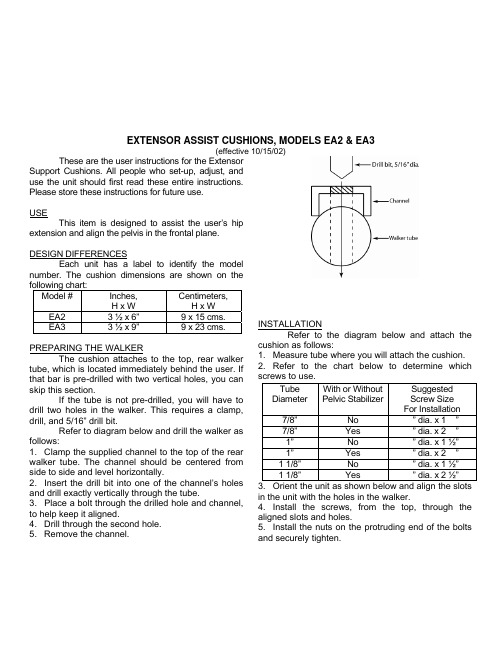
EXTENSOR ASSIST CUSHIONS, MODELS EA2 & EA3(effective 10/15/02)These are the user instructions for the ExtensorSupport Cushions. All people who set-up, adjust, anduse the unit should first read these entire instructions.Please store these instructions for future use.USEThis item is designed to assist the user’s hipextension and align the pelvis in the frontal plane.DESIGN DIFFERENCESEach unit has a label to identify the modelnumber. The cushion dimensions are shown on thefollowing chart:Model # Inches,H x W Centimeters,H x WEA2 3 ½ x 6” 9 x 15 cms. EA3 3 ½ x 9”9 x 23 cms. PREPARING THE WALKERThe cushion attaches to the top, rear walker tube, which is located immediately behind the user. If that bar is pre-drilled with two vertical holes, you can skip this section.If the tube is not pre-drilled, you will have to drill two holes in the walker. This requires a clamp, drill, and 5/16” drill bit.Refer to diagram below and drill the walker as follows:1. Clamp the supplied channel to the top of the rear walker tube. The channel should be centered from side to side and level horizontally.2. Insert the drill bit into one of the channel’s holes and drill exactly vertically through the tube.3. Place a bolt through the drilled hole and channel, to help keep it aligned.4. Drill through the second hole.5. Remove the channel. INSTALLATIONRefer to the diagram below and attach the cushion as follows:1. Measure tube where you will attach the cushion.2. Refer to the chart below to determine which screws to use.3. Orient the unit as shown below and align the slots in the unit with the holes in the walker.4. Install the screws, from the top, through the aligned slots and holes.5. Install the nuts on the protruding end of the bolts and securely tighten.TubeDiameterWith or WithoutPelvic StabilizerSuggestedScrew SizeFor Installation 7/8” No ¼” dia. x 1 ¼”7/8” Yes ¼” dia. x 2 ¼”1” No ¼” dia. x 1 ½”1” Yes ¼” dia. x 2 ¼”1 1/8” No ¼” dia. x 1 ½”1 1/8” Yes ¼” dia. x2 ½”EA2 & EA3 10/15/02, page 2DEPTH ADJUSTMENTTo adjust depth of the cushion:1. Loosen the nuts that attach the unit.2. Slide the unit forward or backward.3. Retighten the nuts.HEIGHT ADJUSTMENTNote: If you have a walker with a fold-down seat, you might not be able to decrease the height of the unit and still fold the seat down.To adjust the height of the unit:1. Loosen the nuts that attach the unit.2. Use a combination of the following two options to adjust the height of the unit:a. For smaller adjustments, attach the unit tothe top of the tube for increased height or to the bottom of the tube for decreased height.b. For larger adjustments, rotate the unit sothat it projects upward for increased height or downward for decreased height.3. Retighten the nuts.MAINTENANCE AND CAREInspect the unit regularly. Tighten the hardware as necessary.If the unit needs service or spare parts, contact Kaye Products, Inc. or the distributor who supplied the unit.If a problem is discovered that may impact the unit’s function, immediately cease use and contact Kaye Products, Inc.Do not expose the unit to rain or submerge it in water.Clean the unit with a damp cloth.Avoid any undue stress to the unit while using, storing, or transporting it.LIMITED WARRANTYIf an item proves defective within two years of the original purchase, we will provide replacement parts in order to correct that defect. Normal wear and tear is not covered by the warranty.Kaye Products, Inc. makes no other warranty, expressed or implied, and does not warrant the product as being fit for a particular purpose. The purchaser, owner, and user assume all risk of personal and property injury due to the use of the equipment. CAUTIONS1. Do not adjust the unit while in use.2. Do not use the unit if there are broken or missing parts.3. Do not alter the unit or use it in any way other than described herein.4. Before use, always ensure that all of the hardware is fully tightened.5. Do not leave the user unattended.6. Use qualified supervision.7. Observe all cautions and size and weight limits for the Kaye Walkers.。
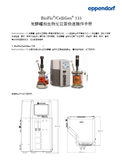
BioFlo-CelliGen 115 中文快速使用手册(Aug 2012)
2第二步:点击pH 第一步:点击Calibration 第三步:输入6.86(或7.0),将电极放入pH6.86(或7.0)的标准缓冲液中,待电极读数稳定后点击“Set Zero”第四步:输入4.0或9.18(或10.0),将电极放入相应的标准缓冲液中,待电极读数稳定后点击“Set Span”2.3 DO 电极的标定(1) 打开DO 电极帽,将电极与缆线相连后连接于主控制台DO 缆线接口进行电极极化,极化时间6小时以上。
(2) 极化完成后,按下图步骤进行标定:(3) 标定零点,如图中第3步,标定有三种方法: 第一种方法:将DO 电极与电极导线断开连接,按图中第三步进行,完成后将电极与缆线重新连接。
第二种方法:需要在标定过程中向培养基中通入氮气,即点击图中“N2 (3) On ”将氮气通入罐内液体中,如果没有“N2(3) On ”选项,可以手动操作通入氮气,随后按图中第三步进行,标定完后点击“N2 (3) Off ”或手动关闭。
第三种方法:将DO 电极置于饱和硫代硫酸钠溶液或饱和亚硫酸钠溶液中,按图中第三步进行。
注意:以上第一、第二种标定方法可在灭菌后标定;第三种方法必须在灭菌前标定0点,灭菌后标定斜率。
(4) 标定斜率,如图中第四步,该标定有两种方式:第一种是将pH 、温度,搅拌转速参数调节至培养所需控制参数值,然 后将通气量调到最大值,待读数稳定后,按图中第四步进行;第二种是将pH 、温度参数调节至培养所需控制参数值,然后将通气量和搅拌转速调到最大值,按图中第四步进行。
注意:DO 斜率标定在灭菌后、接种前进行。
2.4 酸/碱、消泡液和培养基的配制(1) 酸/碱配制根据培养过程要控制的pH 值来确定;一般可选的酸为硫酸、磷酸或通入CO 2来微调pH 值,碱的控制主要为氢氧化钠或NaHCO 3;硫酸,磷酸使用浓度一般最高不超过10%,NaOH 使用浓度一般为1-3 mol/L 。
注意:不要使用盐酸,盐酸会对罐体中金属部件造成腐蚀。
森兰SH100能量回馈单元用户手册
4.1 操作面板的功能..................................................................................................................................9 4.2 操作面板的显示状态和操作 ............................................................................................................10
五、 运输和包装注意事项 不要堆叠超过包装箱规定的堆码数目。 能量回馈单元上面不要放置重物。 当能量回馈单元运输时不要打开盖板。 搬运时,不要让操作面板和盖板受力,否则有人员受伤或财物损失的危险。
六、 报废 按工业垃圾进行处理。 能量回馈单元内部的电解电容焚烧时可能发生爆炸。 能量回馈单元的塑胶件焚烧时会产生有毒气体。
本产品采用的产品技术规范可能发生变化,内容如有改动,恕不另行通知。 本产品用户手册应妥善保存至回馈单元报废为止。
开箱检查注意事项
在开箱时,请认真确认以下项目,如有问题,请直接与本公司或供货商联系解决。
确认项目 与您定购的商品是否一致? 产品是否有破损地方?
型号说明:
确认方法 确认侧面的铭牌内容与您的定货要求是否一致 查看产品整体外观,确认是否在运输中受损
7 保养、维护及售后服务 ..................................................................................................17
Install_cellSens_CH

®安装说明cellSens [Ver.1.12]成像软件该安装指南用于 Olympus cellSens 成像和显微镜数字设备。
为确保安全并获得最佳性能以及您能够熟悉本软件的安装,我们建议您在使用软件前先学习本册。
为了便于以后参考,请将本册存放在方便取用的地方。
以科研与教育为目的本系统是为了科研与教育而设计开发。
目录1重要信息 (4)2安装 cellSens 软件 (7)2-1安装步骤 (8)2-2软件激活 (9)2-2-1软件激活的目的是什么? (9)2-2-2激活步骤 (9)2-2-3什么时候进行软件激活? (10)2-2-4基于 Internet 的软件激活 (11)2-2-5基于文件的软件激活 (12)2-2-6基于代码的软件激活 (16)2-3安装 (18)2-4停用软件 (22)2-4-1基于 Internet 的停用 (23)2-4-2基于文件的停用 (24)2-4-3基于代码的软件停用 (28)2-5激活相关问题的故障排除 (30)2-5-1修复功能 (31)2-5-2恢复功能 (32)3修复功能 (31)4设置显微镜 (34)5卸载 cellSens (37)5-1卸载软件 (37)5-2卸载时的注意事项 (39)6其他 (41)与本说明相关的所有版权均属 Olympus CORPORATION 所有。
Olympus CORPORATION 尽可能使本说明中所包含的信息精确可靠。
尽管如此,Olympus CORPORATION 也不对与本说明相关的任何事项进行任何类型的明示或暗示担保。
未经 Olympus CORPORATION 事先书面允许,本文档的任何部分均不得出于任何目的以任何形式或通过任何手段 (电子或机械) 复制或传输。
商标信息Microsoft 和 Windows 是 Microsoft Corporation, USA 在美国和其它国家/地区的注册商标。
Xsens MTi 1-series 数据手册说明书

MTI-3-8A7G6-DKFeatures▪Full-featured AHRS on 12.1 x 12.1 mm module▪Roll/pitch accuracy (dynamic) 1.0 degFigure 1: MTi 1-seriesTable of ContentsT ABLE OF C ONTENTS (2)1GENERAL INFORMATION (3)1.1O RDERING I NFORMATION (3)1.2B LOCK D IAGRAM (3)1.3T YPICAL A PPLICATION (4)1.4P IN C ONFIGURATION (4)1.5P IN MAP (5)1.6P IN D ESCRIPTIONS (6)1.7P ERIPHERAL INTERFACE SELECTION (6)1.7.1I2C (7)1.7.2SPI (7)1.7.3UART half duplex (7)1.7.4UART full duplex with RTS/CTS flow control (8)1.8R ECOMMENDED EXTERNAL COMPONENTS (8)2MTI 1-SERIES ARCHITECTURE (9)2.1MT I 1-SERIES CONFIGURATIONS (9)2.1.1MTi-1 IMU (9)2.1.2MTi-2 VRU (9)2.1.3MTi-3 AHRS (9)2.2S IGNAL PROCESSING PIPELINE (10)2.2.1Strapdown integration (10)2.2.2XKF3TM Sensor Fusion Algorithm (10)2.2.3Frames of reference used in MTi 1-series (11)33D ORIENTATION AND PERFORMANCE SPECIFICATIONS (12)3.13D O RIENTATION SPECIFICATIONS (12)3.2S ENSORS SPECIFICATIONS (12)4SENSOR CALIBRATION (14)5SYSTEM AND ELECTRICAL SPECIFICATIONS (15)5.1I NTERFACE SPECIFICATIONS (15)5.2S YSTEM SPECIFICATIONS (15)5.3E LECTRICAL SPECIFICATIONS (16)5.4A BSOLUTE MAXIMUM RATINGS (16)6MTI 1-SERIES SETTINGS AND OUTPUTS (17)6.1M ESSAGE STRUCTURE (17)6.2O UTPUT SETTINGS (18)6.3MTD ATA2 (19)6.4S YNCHRONIZATION AND TIMING (20)7MAGNETIC INTERFERENCE (21)7.1M AGNETIC F IELD M APPING (21)7.2A CTIVE H EADING S TABILIZATION (AHS) (21)8PACKAGE AND HANDLING (22)8.1P ACKAGE DRAWING (22)8.2P ACKAGING (23)8.3R EFLOW SPECIFICATION (23)9TRADEMARKS AND REVISIONS (24)9.1T RADEMARKS (24)9.2R EVISIONS (24)Figure 2: MTi 1-series module block diagramFigure 3: Typical application Figure 4: Pin assignmentFigure 8: External components (I2C interface) Figure 9: External components (UART interface)2 MTi 1-series architectureThis section discusses the MTi 1-series architecture including the various configurations and the signal processing pipeline.2.1 MTi 1-series configurationsThe MTi 1-series is a fully-tested self-contained module that can 3D output orientation data (Euler angles (roll, pitch, yaw), rotation matrix (DCM) and quaternions), orientation and velocity increments (∆q and ∆v) and sensors data (acceleration, rate of turn, magnetic field). The MTi 1-series module is available as an Inertial Measurement Unit (IMU), Vertical Reference Unit (VRU) and Attitude and Heading Reference System (AHRS). Depending on the product, output options may be limited to sensors data and/or unreferenced yaw.All MTi’s feature a 3D accelerometer/gyroscope combo-sensor, a magnetometer, a high-accuracy crystal and a low-power MCU. The MCU coordinates the synchronization and timing of the various sensors, it applies calibration models (e.g. temperature modules) and output settings and runs the sensor fusion algorithm. The MCU also generates output messages according to the proprietary XBus communication protocol. The messages and the data output are fully configurable, so that the MTi 1-series limits the load, and thus power consumption, on the application processor.2.1.1 MTi-1 IMUThe MTi-1 module is an Inertial Measurement Unit (IMU) that outputs 3D rate of turn, 3D acceleration and 3D magnetic field. The MTi-1 also outputs coning and sculling compensated orientation increments and velocity increments (∆q and ∆v) from its AttitudeEngine TM. Advantages over a gyroscope-accelerometer combo-sensor are the inclusion of synchronized magnetic field data, on-board signal processing and the easy-to-use communication protocol. Moreover, the testing and calibration performed by Xsens result in a robust and reliable sensor module, that can be integrated within a short time frame. The signal processing pipeline and the suite of output options allow access to the highest possible accuracy at any bandwidth, limiting the load on the application processor.2.1.2 MTi-2 VRUThe MTi-2 is a 3D vertical reference unit (VRU). Its orientation algorithm (XKF3TM) outputs 3D orientation data with respect to a gravity referenced frame: drift-free roll, pitch and unreferenced yaw. In addition, it outputs calibrated sensor data: 3D acceleration, 3D rate of turn and 3D earth-magnetic field data. All modules of the MTi 1-series are also capable of outputting data generated by the strapdown integration algorithm (the AttitudeEngine TM outputting orientation and velocity increments ∆q and ∆v). The3D acceleration is also available as so-called free acceleration which has gravity subtracted. Although the yaw is unreferenced, though still superior to gyroscope integration. With the feature Active Heading Stabilization (AHS, see section 7.2) the drift in unreferenced yaw can be limited to 1 deg after 60 minutes, even in magnetically disturbed environments. 2.1.3 MTi-3 AHRSThe MTi-3 supports all features of the MTi-1 and MTi-2, and in addition is a full gyro-enhanced Attitude and Heading Reference System (AHRS). It outputs drift-free roll, pitch and true/magnetic North referenced yaw and sensors data: 3D acceleration, 3D rate of turn, as well as 3D orientation and velocity increments (∆q and ∆v), and 3D earth-magnetic field data. Free acceleration is also available for the MTi-3 AHRS.2.2 Signal processing pipelineThe MTi 1-series is a self-contained module, so all calculations and processes such as sampling, coning and sculling compensation and the Xsens XKF3TM sensor fusion algorithm run on board.2.2.1 Strapdown integrationThe Xsens optimized strapdown algorithm (AttitudeEngine TM) performs high-speed dead-reckoning calculations at 1 kHz allowing accurate capture of high frequency motions. This approach ensures a high bandwidth. Orientation and velocity increments are calculated with full coning and sculling compensation. At an output data rate of up to 100 Hz, no information is lost, yet the output data rate can be configured low enough for systems with limited communication bandwidth. These orientation and velocity increments are suitable for any 3D motion tracking algorithm. Increments are internally time-synchronized with the magnetometer data.2.2.2 XKF3TM Sensor Fusion AlgorithmXKF3 is a sensor fusion algorithm, based on Extended Kalman Filter framework that uses 3D inertial sensor data (orientation and velocity increments) and 3D magnetometer, also known as ‘9D’ to optimally estimate 3D orientation with respect to an Earth fixed frame.XKF3 takes the orientation and velocity increments together with the magnetic field updates and fuses this to produce a stable orientation (roll, pitch and yaw) with respect to the earth fixed frame. The XKF3 sensor fusion algorithm can be processed with filter profiles. These filter profiles contain predefined filter parameter settings suitable for different user application scenarios.The following filter profiles are available:∙General– suitable for most applications.Supported by the MTi-3 module.∙Dynamic– assumes that the motion is highly dynamic. Supported by the MTi-3 module.∙High_mag_dep– heading corrections rely on the magnetic field measured. To be usedwhen magnetic field is homogeneous.Supported by the MTi-3 module.∙Low_mag_dep– heading corrections are less dependent on the magnetic fieldmeasured. Heading is still based onmagnetic field, but more distortions areexpected with less trust being placed onmagnetic measurements. Supported by theMTi-3 module.∙VRU_general– Roll and pitch are thereferenced to the vertical (gravity), yaw isdetermined by stabilized dead-reckoning,referred to as Active Heading Stabilization(AHS) which significantly reduces headingdrift, see also section 7.2. Consider usingVRU_general in environments that have aheavily disturbed magnetic field. TheVRU_general filter profile is the only filterprofile available for the MTi-2-VRU, alsosupported by the MTi-3 modulezxyFigure 10: Default sensor fixed coordinate system for the MTi 1-series moduleIt is straightforward to apply a rotation matrix to the MTi, so that the velocity and orientation increments, free acceleration and the orientation output is output using that coordinate frame. The default reference coordinate system is East-North-Up (ENU) and the MTi 1-series has predefined output options for North-East-Down (NED) and North-West-Up (NWU). Any arbitrary alignment can be entered. These orientation resets have effect on all outputs that are by default outputted with an ENU reference coordinate system.4 Sensor calibrationEach MTi is individually calibrated and tested over its temperature range. The (simplified) sensor model of the gyroscopes, accelerometers and magnetometers can be represented as following:s=K T−1(u−b T)s = sensor data of the gyroscopes, accelerometers and magnetometers in rad/s, m/s2 or a.u. respectivelyK T-1= gain and misalignment matrix (temperature compensated)u = sensor value before calibration (unsigned 16-bit integers from the sensor)b T= bias (temperature compensated)Xsens’ calibration procedure calibrate s for many parameters, including bias (offset), alignment of the sensors with respect to the module PCB and each other and gain (scale factor). All calibration values are temperature dependent and temperature calibrated. The calibration values are stored in non-volatile memory in the MTi.7 Magnetic interferenceMagnetic interference can be a major source of error for the heading accuracy of any Attitude and Heading Reference System (AHRS). As an AHRS uses the magnetic field to reference the dead-reckoned orientation on the horizontal plane with respect to the (magnetic) North, a severe and prolonged distortion in that magnetic field will cause the magnetic reference to be inaccurate. The MTi 1-series module has several ways to cope with these distortions to minimize the effect on the estimated orientation.7.1 Magnetic Field MappingWhen the distortion is deterministic, i.e. when the distortion moves with the MTi, the MTi can be calibrated for this distortion this type of errors are usually referred to as soft and hard iron distortions. The Magnetic Field Mapping procedure compensates for both hard-iron and soft-iron distortions.In short, the magnetic field mapping (calibration) is performed by moving the MTi together with theobject/platform that is causing the distortion. On an external computer (Windows or Linux), the results are processed and the updated magnetic field calibration values are written to the non-volatile memory of the MTi 1-series module. The magnetic field mapping procedure is extensively documented in the Magnetic Field Mapper User Manual (MT0202P), available in the MT Software Suite. 7.2 Active Heading Stabilization (AHS) It is often not possible or desirable to connect the MTi 1-series module to a high-level processor/host system, so that the Magnetic Field Mapping procedure is not an option. Also, when the distortion is non-deterministic the Magnetic Field Mapping procedure does not yield the desired result. For all these situations, the on-board XKF3 sensor fusion algorithm has integrated an algorithm called Active Heading Stabilization (AHS).The AHS algorithm delivers excellent heading tracking accuracy. Heading tracking drift in the MTi 1-series can be as low as 1 deg per hour, while being fully immune to magnetic distortions.AHS is only available in the VRU_general filter profile. This filter profile is the only filter profile in the MTi-2 VRU and one of the 5 available filter profiles in the MTi-3 AHRS.8 Package and handlingNote that this is a mechanical shock (g) sensitive device. Proper handling is required to prevent damage to the part. Note that this is an ESD-sensitive device. Proper handling is required to prevent damage to the part.8.1 Package drawingThe MTi 1-series module is compatible with JEDEC PLCC28 IC-sockets.Figure 11: General tolerances are +/- 0.1 mmFigure 12: Recommended MTi 1-series module footprint8.2 PackagingThe MTi 1-series module is shipped in trays. Trays are available with a MOQ of 20 modules. A full tray contains 152 modules.Figure 13: A tray containing 20 MTi 1-series modules8.3 Reflow specificationThe moisture sensitivity level of the MTi 1-series modules corresponds to JEDEC MSL Level 3, see also: ∙IPC/JEDEC J-STD-020E “Joint Indus try Standard: Moisture/Reflow Sensitivity Classification for non-hermetic Solid State Surface Mount Devices”∙IPC/JEDEC J-STD-033C “Joint Industry Standard: Handling, Packing, Shipping and Use of Moisture/Reflow Sensitive Surface Mount Devices”.The sensor fulfils the lead-free soldering requirements of the above-mentioned IPC/JEDEC standard, i.e. reflow soldering with a peak temperature up to 260°C. Recommended Preheat Area (t s) is 80-100 sec. The minimum height of the solder after reflow shall be at least 50µm. This is required for good mechanical decoupling between the MTi 1-series module and the printed circuit board (PCB) it is mounted on. Assembled PCB’s may NOT be cleaned with ultrasonic cleaning.MTI-3-8A7G6-DK。
凯米斯仪器有限公司PHG-206在线PH传感器用户手册说明书

PHG-206Online PH SensorUser ManualYANTAI CHEMINS INSTRUMENT CO.,LTD.Tel:*************************E-mail:***********************************************Website:Address:No.15,Entrepreneurship Base,Development Zone,Zhaoyuan City,Shandong Province●Please read the instruction carefully before using and save it for reference.●Please follow the instructions and precautions.●When receiving the instrument,please open the packaging carefully,inspectequipment’s damage level in case of transportation,if you found spoiled equipment,please immediately notify the manufacturer and distributor,and retain the packaging,in order to send back to processing.●When the instrument is in trouble,please don’t repair it by yourself,pleasedirectly contact the maintenance department of the manufacturer.ContentUser Notes (2)Ⅰ、Application Environment (4)Ⅱ、Technical performance and specifications (4)1.Technical parameters (4)2.Dimensional drawing (5)Ⅲ、Installation and electrical connection (5)1.Installation (5)2.Electrical connection (6)Ⅳ、Maintenance and maintenance (6)e and maintenance (6)2.Calibration (7)Ⅴ、Quality and service (7)1.Quality assurance (7)2.Accessories and spare parts (8)3.After-sales service commitment (7)Appendix data communication (8)Ⅰ、Application EnvironmentUsed for environmental water quality monitoring,acid/alkali/salt solution,chemical reaction process and industrial production process,it can meet the requirements of online pH measurement for most industrial applications.●Signal output:RS-485(Modbus/RTU protocol).●Convenient connection to third-party devices such as PLCs,DCS,industrial control computers,general-purpose controllers,paperless recording instruments or touch screens.●Dual high-impedance differential amplifier with strong anti-interference and fast response.●The patented pH probe,the internal reference solution oozes extremely slowly from themicroporous salt bridge at a pressure of at least100kpa(1Bar),and its forward bleedcontinues for more than20months.Such a reference system is very stable and the electrode life is extended by a factor of two compared to conventional industrial electrodes.●Easy to install:3/4NPT pipe thread for easy submersible installation or installation in pipes andtanks.●IP68protection grade.Ⅱ、Technical performance and specifications1.Technical parameters2.Dimensional drawingⅢ、Installation and electrical connection1.InstallationNote:The sensor should not be installed upside down or horizontally when installed,at least at an angle of15degrees or more.2.Electrical connectiona)Red line-power cord(12~24V)b)Black line-ground(GND)c)Blue line-485Ad)white line-485Be)bare wire-shielded wireAfter wiring is completed,it should be carefully checked to avoid incorrect connections before powering up.Cable specification:Considering that the cable is immersed in water(including sea water)for a long time or exposed to the air,the cable has certain corrosion resistance.The outer diameter of the cable isΦ6mm and all interfaces are waterproof.Ⅳ、Maintenance and maintenancee and maintenanceWhen measuring the pH sensor,it should be cleaned in distilled water(or deionized water),and the filter paper should be used to absorb moisture to prevent impurities from being introduced into the liquid to be tested.1/3of the sensor should be inserted into the solution to be tested.The sensor should be washed when not in use,inserted into a protective sleeve with a3.5mol/L potassium chloride solution,or the sensor inserted into a container with a3.5mol/L potassium chloride solution.Check if the terminal is dry.If it is stained,wipe it with absolute alcohol and dry it.Avoid long-term immersion in distilled water or protein solution and prevent contact with silicone grease.With a longer sensor,its glass film may become translucent or with deposits,which can be washed with dilute hydrochloric acid and rinsed with water.The sensor is used for a long time.When a measurement error occurs,it must be calibrated with the meter for calibration.When the calibration and measurement cannot be performed while the sensor is being maintained and maintained in the above manner,the sensor has failed.Please replace the sensor.Standard buffer pH reference tableTemp(℃) 4.00 4.01 6.867.009.1810.010 4.00 4.00 6.987.129.4610.325 4.00 4.00 6.957.099.3910.2510 4.00 4.00 6.927.069.3310.1815 4.00 4.00 6.907.049.2810.1220 4.00 4.00 6.887.029.2310.0625 4.00 4.01 6.867.009.1810.0130 4.01 4.02 6.85 6.999.149.9735 4.02 4.02 6.84 6.989.179.9340 4.03 4.04 6.84 6.979.079.8945 4.04 4.05 6.83 6.979.049.8650 4.06 4.06 6.83 6.979.029.83The actual reading and standard of the instrument sometimes have an error of±1word.2.CalibrationNote:The sensor has been calibrated before leaving the factory.If the measurement error is not exceeded,it should not be arbitrarily calibrated.a)Zero calibrationUse250mL of distilled water in a measuring cylinder,pour into a beaker,add a packet of calibration powder with pH=6.86,stir evenly with a glass rod until the powder is completely dissolved,configure the solution with pH=6.86,put the sensor into the solution,wait for3~5 minutes,after the value is stable,see if the displayed value is6.86.If not,you need to perform zero calibration.Refer to the appendix for the calibration instructions.b)Slope calibrationFor acidic solution:Take250mL of distilled water in a measuring cylinder,pour into a beaker,add a packet of calibration powder with pH=4.00,stir evenly with a glass rod until the powder is completely dissolved,and configure the solution to pH=4.00;In the solution,wait for3to5minutes. After the value is stable,see if the value is4.00.If not,the slope calibration is required.Refer to the appendix for the calibration instructions.For alkaline solution:Take250mL of distilled water in a measuring cylinder,pour into a beaker, add a packet of calibration powder with pH=9.18,stir evenly with a glass rod until the powder is completely dissolved,and configure the solution to pH=9.18;In the solution,wait for3to5minutes. After the value is stable,check if the display is9.18.If not,the slope calibration is required.Refer to the appendix for the calibration instructions.Ⅴ、Quality and service1.Quality assurance●The quality inspection department has standardized inspection procedures,advanced andperfect testing equipment and means,and strictly in accordance with the regulations,to do 72-hour aging test and stability test on the product,and not to allow one unqualified product to leave the factory.●The receiving party directly returns the product batch with a failure rate of2%,and all the costsincurred are borne by the supplier.The reference standard refers to the product description provided by the supplier.●Guarantee the quantity of goods and the speed of shipment.2.Accessories and spare partsThis product includes:●1sensor●Calibration powder3packs●1copy of the manual●1certificate3.After-sales service commitmentThe company provides local after-sales service within one year from the date of sale,but does not include damage caused by improper use.If repair or adjustment is required,please return it, but the shipping cost must be conceited.Damaged on the way,the company will repair the damage of the instrument for free.Appendix data communication1.Data formatThe default data format for Modbus communication is:9600,n,8,1(baud rate9600bps,1start bit,8data bits,no parity,1stop bit).Parameters such as baud rate can be customized.rmation frame formata)Read data instruction frame0603xx xx xx xx xx xx Address Function code Register address Number of registers CRC check code(low byte first)b)Read data response frame0603xx xx......xx xx xxAddress Function code Bytes Answer data CRC check code(low byte first)c)Write data instruction frame0606xx xx xx xx xx xxAddress Function code Register address Write data CRC check code(low byte first)d)Write data response frame(same data command frame)0606xx xx xx xx xx xxAddress Function code Register address Write data CRC check code(low byte first)3.Register addressRegister address Name InstructionNumber ofregistersAccessmethod40001 (0x0000)Measuredvalue+temperature4double-byte integers,which are DO value,DOvalue decimal digits,temperature value,4(8bytes)Reada)The register address defined here is the register address with the type of the register.(Theactual register address is represented in the bracket).b)When address of the device is changed,the response to the data write instruction wouldcontain the new changed address.c)The data definition of the read response value:xx xx xx xx xx xx xx xx2bytes test value2bytes decimal digits*2bytes temp value2bytes decimal digits The default data type is double-byte integer(high byte first),other data format such as floatingpoint type is optional.mand examplea)Read data instructionsFunction:Obtain the pH and temperature of the measuring probe;the unit of pH is pH;the unit of temperature is °C.Request frame:06030000000445BE;Response frame:06030800620002010100012459Example of reading:pH value:0062means hexadecimal reading pH value,0002means pH value with 2decimal places,converted to decimal value 0.98.Temperature value:0101indicates the hexadecimal reading temperature value,0001indicates that the temperature value has 1decimal place and is converted to a decimal value of 25.7.b)Calibration instructionsZero calibrationFunction:Set the pH zero calibration value of the electrode.The zero value is based on the 6.86pH standard.The examples are as follows;Request frame:0606100000008C BD Response frame:0606100000008C BDSlope calibrationFunction:Set the pH slope calibration value of the electrode;the slope calibration is divided into high point and low point calibration,and the alkaline solution is measured at the high point;the acidic solution is measured at the low point,where the standard solution is high here.Point 9.18pH,standard solution low 4.00pH is the calibration reference,examples are as follows:High point standard solution 9.18pH calibration:Request frame:060610040000CD 7C Response frame:060610040000CD 7C Low standard solution 4.00pH calibration:Request frame:0606100200002D 7D Response frame:0606100200002D 7Dc)Set the device ID address:Role:set the MODBUS device address of the electrode;Change the device address 06to 01.The example is as follows Request frame:060620020001E3BDPh value Temperature value0062000201010001烟台凯米斯仪器有限公司11/11 Response frame:060620020001E3BD5.Error responseIf the sensor does not correctly execute the host command,it will return the following format information:Definition Address Function code Code CRC checkData ADDR COM+80H xx CRC 16Number of bytes 1112a)CODE:01–Function code error03–Data is wrongb)COM:The received function code。
希森美康SYSMEX F-820操作手册中文版

目录第一章:概述1. 概述 ························································································································· 1页2. 文件协议 (2)3. 系统特性 (2)4. 系统配置 (5)5. 分析参数 (5)5.1检测原理 (6)6. 画面显示 (7)7. 操作键盘 (8)8. 安全 (9)8.1一般安全 (9)8.2危险性及生物毒性物品 (9)8.3试剂安全 (9)9. 局限性 (10)9.1细胞计数参数 (10)9.2直方图 (12)9.3血红蛋白 (12)第二章:安装1. 安装要求 (12)1.1迁移条件 (12)1.2电源要求 (13)1.3场地要求 (13)1.4环境要求 (13)2. 安装前 (13)2.1拆箱 (13)2.2清点 (14)3. 试剂的连接 (15)3.1护盖的揭开 (15)3.2瓶口插管的安装 (15)3.3稀释液瓶的连接 (15)3.4清洁液瓶的连接 (16)4. 废液瓶 (16)5. 排液管 (17)6. 传感器 (17)6.1传感器及计数孔的冲洗 (17)6.2传感器的镶嵌 (17)7. 管道的充盈 (18)18. HGB组件················································································································ 18页9. 内置打印机 (19)10. 选择性装置 (20)11. 背景检验 (21)12. 数据检查及定标 (21)第二章:样本分析1. 简介 (21)2. 启动程序 (23)2.1操作者检查 (23)2.2电源的开启 (24)2.3自检 (24)2.4准备状态 (24)2.5背景及计数时间的检验 (25)3. 质控物分析 (26)4. 样本准备 (26)4.1样本的收集及处理 (26)4.2样本的稀释 (27)4.3 DB-1样本杯 (30)5. 样本号 (30)6. 样本分析 (30)6.1分析结果的显示 (31)6.2重新计数 (32)7. 分析结果的输出 (33)8. 分析后程序 (34)9. 日常关机 (35)10. 操作者日常检查单 (36)第四章:质量控制1. 简介 (37)2. 质控物的分析 (37)3. QC数据的显示 (38)4. QC数据的输出 (38)4.1内置打印机 (40)4.2外接打印机(选配) (42)4.3主计算机(选配) (43)5. 质控物 (43)2第五章:定标1. 简介 ······················································································································· 43页2. 定标频率 (44)3. 参考物及方法 (44)3.1定标样本 (44)3.2 Sysmex定标物 (44)3.3参考方法学 (44)3.4参考程序 (44)4. 自动定标 (45)4.1 HGB (46)4.2 HCT (50)4.3 HGB/HCT (51)5. 手工定标 (53)5.1样本分析 (53)5.2新补偿值的计算 (53)5.3新定标值的输入 (54)5.4样本的重新分析 (55)第六章:储存的数据1. 简介 (56)2. 储存数据的显示 (56)3. 储存数据的输出 (57)3.1内置打印机 (57)3.2外接打印机(选配) (59)3.3主计算机(选配) (61)4. 储存数据的清除 (64)4.1按行清除 (64)4.2所有的储存数据的清除 (66)第七章:手工甄别1. 简介 (68)2. WBC (68)3. RBC (69)4. PLT (71)第八章:保养及调校1. 简介 (74)2. F-820保养清单 (74)3. 定期保养 (75)3.1废液瓶的检查 (75)3.2废液的排弃 (75)3.3 HGB水路系统的清洗 (76)34. 按需保养 ················································································································· 76页4.1计数孔的清洗 (76)4.2液晶屏幕(LCD)的清洁 (77)4.3传感器的清洗 (77)4.4真空罐内液的排放 (78)4.5 HGB管道堵塞的排除 (78)5. 调较 (79)5.1 HGB检测电路的调校 (79)5.2 HGB样本吸量的调校 (80)5.3液晶萤屏亮度及对比度的调校 (80)6. 配件的更换 (81)6.1试剂瓶的更换 (81)6.2系统保险丝的更换 (81)6.3 HGB灯泡的更换 (82)6.4内置打印机的供纸 (83)7. 零配件清单 (86)第九章:故障的检修 (87)1. 简介 (87)2. 按故障代号检修 (87)2.1故障号(按字母顺序编排) (88)3. 故障号注释 (88)4. 系统保养(无故障号) (95)5. 异常结果的检查 (95)5.1 RBC/PLT/HCT—重复性差 (96)5.2 RBC/PCT/HCT—计数编高 (97)5.3 RBC/PLT/HCT—计数编低 (98)5.4 WBC—重复性差 (99)5.5 WBC—计数编高 (100)5.6 WBC—计数编低 (101)5.7 HGB—重复性差 (102)5.8 HGB—结果编高 (102)5.9 HGB—结果编低 (102)6. 测试程序 (103)6.1 HGB组件 (103)6.2内置打印机 (104)6.3外接打印机 (105)6.4主计算机 (106)4第十章:功能介绍1. 简介 ······················································································································ 107页2. 细胞计算原理 (107)2.1检测原理 (107)2.2操作顺序 (108)2.3噪音脉冲的监测 (110)3. 测量原理 (110)3.1 HGB (110)3.2 HCT (111)3.3 MCV/MCH/MCHC (111)4. 颗粒大小分布的分析 (111)4.1 WBC颗粒大小的分布 (112)4.2 RBC颗粒大小的分布 (112)4.3 PLT颗粒大小的分布 (114)5. 操作者的控制及提示 (115)5.1前方 (115)5.2传感器 (116)5.3后方 (116)5.4水路连接器 (117)5.5 HGB组件 (118)第十一章:系统设置1. 简介 (119)2. 病人异常结果的提示界限 (119)3. PLT重新计数限制 (121)4. X—轴尺度 (122)5. 日期/时间 (123)6. 输出格式 (124)6.1内置打印机 (124)6.2外接打印机 (125)6.3主计算机 (127)第十二章:技术资料1. DIP转换设置 (129)1.1输出设置(DIP-1) (130)1.2数据格式/分析参数(D1P-2) (130)1.3语言(ROTARY-1) (130)1.4单位(ROTARY-2) (131)52. 主计算机的串连接口································································································· 132页2.1连接 (132)2.2输入/输出信号 (132)2.3通信方式 (132)2.4波特率/字符结构 (132)2.5信号电平 (132)2.6软件 (132)3. 内容格式 (133)3.1样本数据格式 (133)3.2质控数据格式 (136)4. 打印卡规格 (137)5. 扩展程序的设置 (137)5.1堵塞报警时间 (138)5.2 HBG吸量时间 (138)5.3组件操作的手工开/闭 (139)附录A:菜单分析图 (141)6第一章概述1.概观Sysmex F-820 是一部用于临床实验室体外诊断的半自动血液分析仪。
- 1、下载文档前请自行甄别文档内容的完整性,平台不提供额外的编辑、内容补充、找答案等附加服务。
- 2、"仅部分预览"的文档,不可在线预览部分如存在完整性等问题,可反馈申请退款(可完整预览的文档不适用该条件!)。
- 3、如文档侵犯您的权益,请联系客服反馈,我们会尽快为您处理(人工客服工作时间:9:00-18:30)。
4. 采集单幅图像 .......................................................16
4.1. 拍照....................................................................... 16 4.2. 活动窗口的行为 ............................................................. 17 4.3. 采集 HDR 图像.............................................................. 19
10.1.1. 测量多通道 Z 图像栈上的亮度剖线 ................................. 60 10.1.2. 测量移动对象的亮度剖线 .......................................... 63
10.2.
记波器................................................................... 65
10.2.1. 周期性移动的视觉展示 ............................................ 66 10.2.2. 在...................... 68
10.3.
荧光分解................................................................. 71
采集多个单幅荧光图像 ............................................ 39 组合通道 ........................................................ 40
7.5. 采集多通道荧光图像 ......................................................... 44
用户手册
cellSens 1.14
LIFE SCIENCE IMAGING SOFTWARE
与本手册相关的所有版权均属 Olympus CORPORATION 所有。 Olympus CORPORATION 尽可能使本手册中所包含的信息精确可靠。尽管如此,Olympus CORPORATION
不对与本手册相关的任何事项进行任何类型的明示或暗示担保,包括但不限于任何特定目的的适 销性或适用性。Olympus CORPORATION 将会经常对本手册中描述的软件进行修正,并保留无责任 对购买者另行通知所做更改的权利。在任何情况下,Olympus CORPORATION 将不会对由于购买或
Version 510_UMA_cellSens114-Orinoco_chs_00
目录
1. 关于本软件文档 ......................................................6
2. 用户界面简介 ........................................................7
7.3. 定义荧光采集的观测模式 ..................................................... 35
7.4. 采集和组合荧光图像 ......................................................... 39
7.4.1. 7.4.2.
10.6.
比例分析................................................................. 83
10.6.1. 总览 ............................................................ 83 10.6.2. 执行比例分析 .................................................... 85
8. 创建拼接图像 .......................................................49
8.1. 什么是拼接图像? ............................................................ 49
8.2. 在不使用电动 XY 扫描台的情况下采集拼接图像 (手动图像拼接) .................. 49 8.2.1. 使用电动 XY 扫描台采集拼接图像 (XY 位置 / 图像拼接) ............. 52
10.3.1. 总览 ............................................................ 71 10.3.2. 执行荧光分解 .................................................... 73
10.4.
10.5. 消卷积................................................................... 81 10.5.1. 总览 ............................................................ 81
6.1.
时间栈..................................................................... 24
6.1.1. 6.1.2. 6.1.3. 6.1.4.
什么是时间栈? ................................................... 24 缩时/录像 ....................................................... 25 采集录像 ........................................................ 25 采集时间栈 ...................................................... 26
使用本手册及其所包含的信息所造成的间接、特例、偶发或伴随发生的任何损害承担责任。
未经 Olympus CORPORATION 事先书面允许,本文档的任何部分均不得出于任何目的以任何形式或通 过任何手段 (电子或机械) 复制或传输。
所有品牌均为各自所有者的商标或注册商标。
© OLYMPUS CORPORATION 保留所有权利
12. 测量图像 ........................................................98
共定位................................................................... 76
10.4.1. 什么是共定位? ................................................... 76 10.4.2. 共定位测量 ...................................................... 76
2.1. 用户界面.................................................................... 7 2.2. 布局........................................................................ 8 2.3. 文档组...................................................................... 9 2.4. 工具窗口................................................................... 10 2.5. 图像窗口视图............................................................... 11 2.6. 使用文档................................................................... 12
9. 处理图像 ...........................................................57
10. 生命科学应用 ....................................................58
10.1.
亮度剖线................................................................. 59
5. 采集多维图像 .......................................................21
5.1. 简介 - 采集流程 ............................................................ 22
6. 采集图像序列 .......................................................24
8.3. 使用扩展焦距采集拼接图像 ................................................... 54
8.4. 自动采集多个拼接图像 ....................................................... 55