Ansys Fluent 13.0 or 14.0 Tutorials教程
Windows7系统下ANSYS_Fluent14.0多机并行安装及启动设置

Windows7系统下ANSYS_Fluent14.0多机并行安装及启动设置关于ANSYS_Fluent14.0的多机并行安装及设置,网上没有详细的介绍,有的也是比较早的版本。
经过几天的反复摸索,终于完成并行安装及设置,为了避免遗忘,现把安装及设置过程记录下来。
1. 关于多机并行和单机多核并行单机多核并行,即一台机器多核处理器,进行并行计算,这个大多数都能比较轻松实现,再次不在详述。
多机并行,即多个电脑并行起来,其中一台电脑作为主机,其他电脑为副机,实现多台电脑的计算集群达到并行计算的效果。
2. 安装软件,版本为ANSYS_Fluent14.0(其他版本未测试)在每台计算机的相同目录下安装ANSYS,如D:\Program Files\ANSYS Inc;具体软件安装过程可以参照网上的教程,自己搜索下……其中,第三步也需要安装,即Install MPI for ANSYS Inc,Parallel Processing,其中包括两个MPI版本,分别为Intel MPI和Platform MPI,分别安装即可。
3. 设置共享分别将Fluent的安装目录和工作目录设置共享,具体方法自己百度吧……设置共享需要达到的效果如下图:即彼此可以看到对方,并且可以访问对方设置共享的文件夹。
为了访问方便,在设置共享时尽量把共享的权限降低。
4. 分别在主机和副机上建立用户名和密码相同的账户,即公共账户。
5. MPI设置(分别在主机和副机上设置)1) 通过命令提示符cmd将目录设置在:D:\Program Files\ANSYS Inc\v140\fluent\ntbin\win64目录下,运行rshd -install,安装rshd;2) 通过命令提示符cmd将目录设置在:D:\Program Files\ANSYS Inc\v140\fluent\fluet14.0.0\multiport\win64\intel\bin目录下,运行smpd -install,安装smpd;3) 在D:\Program Files\ANSYS Inc\v140\fluent\fluet14.0.0\multiport\win64\intel\bin目录下,找到wmpiregister,将公共账户和密码设置如下图6. ANSYS Fluent14.0启动设置1) 打开ANSYS Fluent14.0如下图:工作目录设置为之前建立的共享工作目录,如\\TAN-PC\fluent-work;FLUENT启动目录为D:\Program Files\ANSYS Inc\v140\fluent\; (无需设置,自动显示) Processing Options处,Parallel per Machine File machine, Number of Process处设置启动核数;2) Parallel Settings设置如下图:MPI类型处,选择intel ;Run Types处,选择Distributed Memory on Local Machine.3) 点击OK和Yes,忽略两个警告信息后成功启动多机并行Fluent。
ansysfluent13.0or14.0tutorials教程
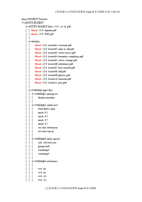
Ansys FLUENT Tutorials└─ANSYS FLUENT├─ANSYS-FLUENT-Intro_13.0_1st-ed_pdf││fluent_13.0_Agenda.pdf││fluent_13.0_TOC.pdf│││├─lectures││fluent_13.0_lecture01-welcome.pdf││fluent_13.0_lecture02-intro-to-cfd.pdf││fluent_13.0_lecture03-solver-basics.pdf││fluent_13.0_lecture04-boundary-conditions.pdf ││fluent_13.0_lecture05-solver-settings.pdf││fluent_13.0_lecture06-turbulence.pdf││fluent_13.0_lecture07-heat-transfer.pdf││fluent_13.0_lecture08-udf.pdf││fluent_13.0_lecture09-physics.pdf││fluent_13.0_lecture10-transient.pdf││fluent_13.0_lecture11-post.pdf│││├─workshop-input-files││├─workshop1-mixing-tee│││ fluidtee.meshdat│││││├─workshop2-airfoil-new│││ NACA0012.msh│││ mach_0.5_│││ mach_0.5_│││ mach_0.7_│││ mach_0.7_│││ test-data-bottom.xy│││ test-data-top.xy│││││├─workshop3-multi-species│││ calc_activities.jou│││ garage.msh│││ workshop3-│││ workshop3-│││││├─workshop4-electronics││││││ ws4_no-│││ ws4_no-│││ ws4_s2s-│││ ws4_s2s-│││││├─workshop5-moving-parts│││ ws5-mesh-animation.avi│││ ws5-simple-wind-turbine.msh│││ ws5_udf_for_motion.c│││││├─workshop6-dpm│││ dpm_tutorial.msh│││││└─workshop7-tank-flush││││ws7-tankflush-animation.avi││ws7-tankflush-animation.mpeg│││└─workshops│fluent_13.0_WS_TOC.pdf│fluent_13.0_workshop01-mixingtee.pdf│fluent_13.0_workshop02-airfoil.pdf│fluent_13.0_workshop03-Multiple-Species.pdf│fluent_13.0_workshop04-electronics.pdf│fluent_13.0_workshop05-moving-parts.pdf│fluent_13.0_workshop06-dpm.pdf│fluent_13.0_workshop07-tank-flush.pdf│├─Quick Tutorials││ FLUENT_Overview_1_Introduction_to_FLUENT12_in_ANSYS_Workbench_DOC.pd f││ FLUENT_Overview_1_Introduction_to_FLUENT12_in_ANSYS_Workbench_WA TCH ME.swf││ FLUENT_Overview_2_Creating_and_Comparing_Related_FLUENT12_Analyses_in_ ANSYS_Workbench_DOC.pdf││ FLUENT_Overview_2_Creating_and_Comparing_Related_FLUENT12_Analyses_in_ ANSYS_Workbench_WA TCHME.swf││ FLUENT_Overview_3_Parametric_Study_Using_FLUENT12_in_ANSYS_Workbench _DOC.pdf││ FLUENT_Overview_3_Parametric_Study_Using_FLUENT12_in_ANSYS_Workbench _WATCHME.swf││ FLUENT_Overview_4_1-Way_Fluid-Structure_Interaction_Using_FLUENT12_and_A NSYS_Mechanical_DOC.pdf││ FLUENT_Overview_4_1-Way_Fluid-Structure_Interaction_Using_FLUENT12_and_A NSYS_Mechanical_WA TCHME.swf│││├─FLUENT_Overview_1_FILES│││├─FLUENT_Overview_2_FILES│││ Duplicate_Probe_Fluent.wbpj │││││└─Duplicate_Probe_Fluent_files │││ .project_cache│││││├─dp0││││ designPoint.wbdp│││││││├─FFF││││├─DM│││││ FFF.agdb│││││││││├─Fluent│││││ FFF-1-│││││ FFF-│││││ FFF.set│││││││││├─MECH│││││ FFF.msh│││││││││└─Post││││Probe.cst│││││││├─FFF-1││││└─Fluent││││FFF-1.1-1-│││││││└─global│││└─MECH││││ FFF.mshdb│││││││└─FFF││└─user_files│├─FLUENT_Overview_3_FILES│││ Parametric_Probe_Fluent.wbpj │││││└─Parametri c_Probe_Fluent_files │││ .project_cache│││││├─dp0││││ designPoint.wbdp│││││││├─FFF││││├─DM│││││ FFF.agdb│││││││││├─Fluent│││││ FFF-1-│││││ FFF-│││││ FFF.set│││││││││├─MECH│││││ FFF.msh│││││││││└─Post││││Probe.cst│││││││├─FFF-1││││└─Fluent││││FFF-1.1-1- │││││││└─global│││└─MECH││││ FFF.mshdb │││││││└─FFF││└─user_files│└─FLUENT_Overview_4_FILES ││ FSI_Probe_Fluent.wbpj│││└─FSI_Probe_Fluent_files││ .project_cache│││├─dp0│││ designPoint.wbdp │││││├─FFF│││├─DM││││ FFF.agdb│││││││├─Fluent││││ FFF-1-││││ FFF-││││ FFF.set│││││││├─MECH││││ FFF.msh│││││││└─Post│││Probe.cst│││││├─FFF-1│││└─Fluent│││FFF-1.1-1-│││││└─global││└─MECH│││ FFF.mshdb│││││└─FFF│└─user_files├─combustion-fluent││ combustion-tutorial-list_││ tut-01-intro-tut-16-species-transport.pdf││ tut-02-intro-tut-17-non-premix-combustion.pdf ││ tut-03-intro-tut-18-surface-chemistry.pdf││ tut-04-intro-tut-19-evaporating-liquid.pdf││ tut-05-berl.pdf││ tut-06-finite-rate.pdf││ tut-07-pdf-jet.pdf││ tut-08-cijr.pdf││ tut-09-pilot-jet.pdf││ tut-10-zimont.pdf││ tut-11-surfchem.pdf││ tut-12-mchar.pdf││ tut-13-co-combustor.pdf││ tut-14-flamelet.pdf││ tut-15-moss-brookes.pdf││ tut-16-dqmom.pdf││ tut-17-species.pdf││ tut-18-euler-granular.pdf││ tut-19-dpm-channel.pdf│││├─tut-01-intro-tut-16-species-transport│││ gascomb.msh│││││└─solution_files│││││││││││││││├─tut-02-intro-tut-17-non-premix-combustion │││ berl.msh│││ berl.prof│││││└─solution_files││berl-││berl-││berl.pdf│││├─tut-03-intro-tut-18-surface-chemistry│││ surface.msh│││││└─solution_files││surface-non-││surface-││surface-││surface-││surface-│││├─tut-04-intro-tut-19-evaporating-liquid│││ sector.msh│││││└─solution_files││sector.msh│││││││││││││││├─tut-05-berl││││││ berl.prof│││││└─solution_files││berl-mag-││berl-mag-││berl-mag-││berl-mag-││berl-mag-││berl-mag-│││├─tut-06-finite-rate││││││││└─solution_files││││││5step_││5step_││5step_│││├─tut-07-pdf-jet│││ CH4-skel.che││││││ therm.dat│││││└─solution_files││flameD-││flameD-││flameD-││flameD-││flameD-││flameD-││││surf-mon-1.out │││├─tut-08-cijr│││ CIJR-therm.dat│││ CIJR.che││││││││└─solution_files││CIJR-││CIJR-││CIJR-││CIJR-││CIJR-││CIJR-││CIJR-││CIJR-││CIJR-│││││││││││├─tut-09-pilot-jet│││ flameD-│││ gri30.che│││││└─solution_files││flameD-sfla- ││flameD-sfla- ││flameD-││flameD-││flameD-ufla- ││flameD-ufla- ││flameD-ufla- ││surf-mon-1.out │││├─tut-10-zimont│││ conreac.msh│││││└─solution_files││zimont-││zimont-││zimont-││zimont-│││││├─tut-11-surfchem│││ gas_chem.che│││ surf_chem.che││││││││└─solution_files││surf-cat-││surf-cat-││surf-mon-1.out │││├─tut-12-mchar││││││││└─solution_files││mchar-││mchar-││││││view-0.vw│││├─tut-13-co-combustor│││ par-│││││└─solution_files││par-││peters-partially-premixed- ││peters-partially-premixed- ││zimont-partially-premixed- ││zimont-partially-premixed- ││zimont-partially-premixed- ││zimont-partially-premixed- ││zimont-partially-││zimont-partially-│││├─tut-14-flamelet││││││ berl.prof│││ smooke46.che│││ thermo.db│││││└─sol ution_files││berl-││berl-││berl-││berl-││berl-│││││││├─tut-15-moss-brookes│││ brookes_│││ brookes_│││ brookes_│││ brookes_ch4.ray│││ flamlet.fla│││ therm.dat│││││└─solution_files││brookes_ch4_soot_││brookes_ch4_soot_│││├─tut-16-dqmom││││││││└─solution_files││dqmom-││dqmom-││dqmom-││dqmom-││dqmom-││dqmom-││dqmom-││dqmom-│││││││├─tut-17-species│││ baffled_│││││└─solution_files││case-1-rtd-││case-1-rtd-││case-1-tracer-││case-1-tracer-││case-1-tracer-injection- ││case-1-tracer-injection- ││case-1-tracer.out││case-││case-││case-2-rtd-││case-2-rtd-││case-2-rtd-││case-2-rtd-││case-2-tracer-││case-2-tracer-││case-2-tracer-injection- ││case-2-tracer-injection- ││case-2-tracer.out││case-││case-││surf-mon-1.out│││├─tut-18-euler-granular││││││ mass_xfer_rate.c│││││└─solution_files││euler-gran-││euler-gran-││euler-gran-││euler-gran-││vol-solid.out│││└─tut-19-dpm-channel│││││└─solution_files│ dpm-│ dpm-│ pipe-│ pipe-│├─extra││ FLUENT13_workshop_XX_RAE_Airfoil.pptx ││ FLUENT13_workshop_XX_V ortexShedding.pptx │││├─workshop_XX_RAE_Airfoil│││ ExperimentalData.csv│││ coarse.xy│││ experiment.xy│││ expressions.cst│││ rae2822_coarse.msh│││││└─Result_TUT_04│││ rae2822_coarse-data_export_to_post.cas │││ rae2822_coarse-data_export_to_post.cdat │││ rae2822_coarse-data_export_to_post.cst│││ rae2822_│││ rae2822_│││││└─FINE_MESH││ medium.xy││ rae2822_││ rae2822_││ rae2822_fine.msh││ rae2822_││ rae2822_││ rae2822_medium.msh│││└─workshop_XX_V ortexShedding││ point-4-y-velocity-final.out││ vortex-shedding-coarse.msh││ vortex-shedding-││ vortex-shedding-│││├─FILES_FOR_CFDPOST││ vectors.mp4││ vortex-shedding-unsteady-3- ││ vortex-shedding-unsteady-3- ││ vortex-shedding-unsteady-3- ││ vortex-shedding-unsteady-3- ││ vortex-shedding-unsteady-3- ││ vortex-shedding-unsteady-3- ││ vortex-shedding-unsteady-3- ││ vortex-shedding-unsteady-3- ││ vortex-shedding-unsteady-3- ││ vortex-shedding-unsteady-3- ││ vortex-shedding-unsteady-3- ││ vortex-shedding-unsteady-3- ││ vortex-shedding-unsteady-3- ││ vortex-shedding-unsteady-3- ││ vortex-shedding-unsteady-3- ││ vortex-shedding-unsteady-3- ││ vortex-shedding-unsteady-3- ││ vortex-shedding-unsteady-3- ││ vortex-shedding-unsteady-3- ││ vortex-shedding-unsteady-3- ││ vortex-shedding-unsteady-3- ││ vortex-shedding-unsteady-3- ││ vortex-shedding-unsteady-3- ││ vortex-shedding-unsteady-3- ││ vortex-shedding-unsteady-3- ││ vortex-shedding-unsteady-3- ││ vortex-shedding-unsteady-3- ││ vortex-shedding-unsteady-3- ││ vortex-shedding-unsteady-3- ││ vortex-shedding-unsteady-3- ││ vortex-shedding-unsteady-3- ││ vortex-shedding-unsteady-3- ││ vortex-shedding-unsteady-3- ││ vortex-shedding-unsteady-3-││ vortex-shedding-unsteady-3- ││ vortex-shedding-unsteady-3- ││ vortex-shedding-unsteady-3- ││ vortex-shedding-unsteady-3- ││ vortex-shedding-unsteady-3- ││ vortex-shedding-unsteady-3- ││ vortex-shedding-unsteady-3- ││ vortex-shedding-unsteady-3- ││ vortex-shedding-unsteady-3- ││ vortex-shedding-unsteady-3- ││ vortex-shedding-unsteady-3- ││ vortex-shedding-unsteady-3- ││ vortex-shedding-unsteady-3- ││ vortex-shedding-unsteady-3- ││ vortex-shedding-unsteady-3- ││ vortex-shedding-unsteady-3- ││ vortex-shedding-unsteady-3- ││ vortex-shedding-unsteady-3- ││ vortex-shedding-unsteady-3- ││ vortex-shedding-unsteady-3- ││ vortex-shedding-unsteady-3- ││ vortex-shedding-unsteady-3- ││ vortex-shedding-unsteady-3- ││ vortex-shedding-unsteady-3- ││ vortex-shedding-unsteady-3- ││ vortex-shedding-unsteady-3- ││ vortex-shedding-unsteady-3- ││ vortex-shedding-unsteady-3- ││ vortex-shedding-unsteady-3- ││ vortex-shedding-unsteady-3- ││ vortex-shedding-unsteady-3- ││ vortex-shedding-unsteady-3- ││ vortex-shedding-unsteady-3- ││ vortex-shedding-unsteady-3- ││ vortex-shedding-unsteady-3- ││ vortex-shedding-unsteady-3- ││ vortex-shedding-unsteady-3- ││ vortex-shedding-unsteady-3- ││ vortex-shedding-unsteady-3- ││ vortex-shedding-unsteady-3- ││ vortex-shedding-unsteady-3- ││ vortex-shedding-unsteady-3- ││ vortex-shedding-unsteady-3-││ vortex-shedding-unsteady-3- ││ vortex-shedding-unsteady-3- ││ vortex-shedding-unsteady-3- ││ vortex-shedding-unsteady-3- ││ vortex-shedding-unsteady-3- ││ vortex-shedding-unsteady-3- ││ vortex-shedding-unsteady-3- ││ vortex-shedding-unsteady-3- ││ vortex-shedding-unsteady-3- ││ vortex-shedding-unsteady-3- ││ vortex-shedding-unsteady-3- ││ vortex-shedding-unsteady-3- ││ vortex-shedding-unsteady-3- ││ vortex-shedding-unsteady-3- ││ vortex-shedding-unsteady-3- ││ vortex-shedding-unsteady-3- ││ vortex-shedding-unsteady-3- ││ vortex-shedding-unsteady- │││└─Result-TUT_07││ cfd_post.cst││ point-4-y-velocity-final.out ││ point-4-y-velocity.out││ sequence-1.mpeg││ vectors.mp4││ vortex-shedding-coarse-││ vortex-shedding-coarse-││ vortex-shedding-unsteady- ││ vortex-shedding-unsteady- ││ vortex-shedding-││ vortex-shedding-│││├─ADDITIONAL-FILES││ q-criterion2D.scm││ velocity.fft│││└─ANIMATION-FILES│ sequence-1.cxa│ sequence-1.mpeg│ sequence-1_0000.hmf│ sequence-1_0001.hmf│ sequence-1_0002.hmf│ sequence-1_0003.hmf│ sequence-1_0005.hmf │ sequence-1_0006.hmf │ sequence-1_0007.hmf │ sequence-1_0008.hmf │ sequence-1_0009.hmf │ sequence-1_0010.hmf │ sequence-1_0011.hmf │ sequence-1_0012.hmf │ sequence-1_0013.hmf │ sequence-1_0014.hmf │ sequence-1_0015.hmf │ sequence-1_0016.hmf │ sequence-1_0017.hmf │ sequence-1_0018.hmf │ sequence-1_0019.hmf │ sequence-1_0020.hmf │ sequence-1_0021.hmf │ sequence-1_0022.hmf │ sequence-1_0023.hmf │ sequence-1_0024.hmf │ sequence-1_0025.hmf │ sequence-1_0026.hmf │ sequence-1_0027.hmf │ sequence-1_0028.hmf │ sequence-1_0029.hmf │ sequence-1_0030.hmf │ sequence-1_0031.hmf │ sequence-1_0032.hmf │ sequence-1_0033.hmf │ sequence-1_0034.hmf │ sequence-1_0035.hmf │ sequence-1_0036.hmf │ sequence-1_0037.hmf │ sequence-1_0038.hmf │ sequence-1_0039.hmf │ sequence-1_0040.hmf │ sequence-1_0041.hmf │ sequence-1_0042.hmf │ sequence-1_0043.hmf │ sequence-1_0044.hmf │ sequence-1_0045.hmf │ sequence-1_0046.hmf │ sequence-1_0047.hmf│ sequence-1_0049.hmf │ sequence-1_0050.hmf │ sequence-1_0051.hmf │ sequence-1_0052.hmf │ sequence-1_0053.hmf │ sequence-1_0054.hmf │ sequence-1_0055.hmf │ sequence-1_0056.hmf │ sequence-1_0057.hmf │ sequence-1_0058.hmf │ sequence-1_0059.hmf │ sequence-1_0060.hmf │ sequence-1_0061.hmf │ sequence-1_0062.hmf │ sequence-1_0063.hmf │ sequence-1_0064.hmf │ sequence-1_0065.hmf │ sequence-1_0066.hmf │ sequence-1_0067.hmf │ sequence-1_0068.hmf │ sequence-1_0069.hmf │ sequence-1_0070.hmf │ sequence-1_0071.hmf │ sequence-1_0072.hmf │ sequence-1_0073.hmf │ sequence-1_0074.hmf │ sequence-1_0075.hmf │ sequence-1_0076.hmf │ sequence-1_0077.hmf │ sequence-1_0078.hmf │ sequence-1_0079.hmf │ sequence-1_0080.hmf │ sequence-1_0081.hmf │ sequence-1_0082.hmf │ sequence-1_0083.hmf │ sequence-1_0084.hmf │ sequence-1_0085.hmf │ sequence-1_0086.hmf │ sequence-1_0087.hmf │ sequence-1_0088.hmf │ sequence-1_0089.hmf │ sequence-1_0090.hmf │ sequence-1_0091.hmf│ sequence-1_0093.hmf│ sequence-1_0094.hmf│ sequence-1_0095.hmf│ sequence-1_0096.hmf│ sequence-1_0097.hmf│ sequence-1_0098.hmf│ sequence-1_0099.hmf│ sequence-1_0100.hmf│ sequence-1_0101.hmf│ sequence-1_0102.hmf│ sequence-1_0103.hmf│ sequence-1_0104.hmf│ sequence-1_0105.hmf│ sequence-1_0106.hmf│ sequence-1_0107.hmf│ sequence-1_0108.hmf│ sequence-1_0109.hmf│ sequence-1_0110.hmf│ sequence-1_0111.hmf│ sequence-1_0112.hmf│ sequence-1_0113.hmf│ sequence-1_0114.hmf│ sequence-1_0115.hmf│ sequence-1_0116.hmf│ sequence-1_0117.hmf│ sequence-1_0118.hmf│ sequence-1_0119.hmf│├─fluent-heat-transfer││ ht-01-intro-tut-04-periodic-flow-heat.pdf││ ht-02-intro-tut-07-radiation-and-convection.pdf ││ ht-03-intro-tut-08-DO-radiation.pdf││ ht-04-intro-tut-24-solidification.pdf││ ht-05-conjugate-heat-transfer.pdf││ ht-06-compact-heat-exchanger.pdf││ ht-07-macro-heat-exchanger.pdf││ ht-08-head-lamp.pdf│││├─ht-01-intro-tut-04-periodic-flow-heat│││ tubebank.msh│││││└─solution_files│││││││├─ht-02-intro-tut-07-radiation-and-convection ││││││││└─solution_files││rad_││rad_││rad_││rad_││rad_││rad_││rad_││rad_││rad_││rad_││rad_││rad_││rad_││rad_││rad_││rad_││rad_a_││rad_b_││rad_b_││rad_││rad_││rad_││tp_1.xy││tp_10.xy││tp_100.xy││tp_1600.xy││tp_400.xy││tp_800.xy││tp_partial.xy│││├─ht-03-intro-tut-08-DO-radiation││││││││└─solution_files││││││do_2x2_10x10_││do_2x2_10x10_││do_2x2_10x10_pix.xy││do_2x2_1x1.xy││do_2x2_2x2_││do_2x2_2x2_││do_2x2_2x2_pix.xy││do_2x2_3x3_││do_2x2_3x3_││do_2x2_3x3_div.xy││do_2x2_3x3_││do_2x2_3x3_││do_2x2_3x3_pix.xy││do_3x3_3x3_││do_3x3_3x3_││do_3x3_3x3_div.xy││do_3x3_3x3_div_baf_int.xy ││do_3x3_3x3_div_││do_3x3_3x3_div_││do_3x3_3x3_div_df=1.xy ││do_3x3_3x3_div_││do_3x3_3x3_div_││do_5x5_3x3_││do_5x5_3x3_││do_5x5_3x3_div.xy│││├─ht-04-intro-tut-24-solidification│││ solid.msh│││││└─solution_files│││││││││││││││││││├─ht-05-conjugate-heat-transfer││││││││└─solution_files││chip3d-││chip3d-││chip3d-││chip3d-││││││surf-mon-1.out││temp-0.xy││temp-1.xy││temp-2.xy││velocity-0.xy││velocity-1.xy││velocity-2.xy││xwss-0.xy││xwss-1.xy││xwss-2.xy│││├─ht-06-compact-heat-exchanger ││││││││└─solution_files││htx-││htx-││htx-││htx-││htx-││htx-││htx-││htx-││surf-mon-1.out│││├─ht-07-macro-heat-exchanger │││ rad.tab││││││││└─solution_files│││││││││││││││││││└─ht-08-head-lamp││ head-│││└─solution_files│ auto-│ auto-│ head-lamp-t.out│ hed-lamp-v.out│├─multiphase-fluent││ 01-hfilm.pdf││ 02-boil.pdf││ 03-nucleate_boil.pdf││ 04-dambreak.pdf││ 05-sloshing.pdf││ 06-bubble-col.pdf││ 07-bubble-break.pdf││ 08-inkjet.pdf││ 09-sparger.pdf││ 10-pbed-reactor.pdf││ 11-ddpm.pdf││ 12-dm-ship-wave.pdf││ 13-udf-clarifier.pdf││ 14-udf-fbed.pdf│││├─tut-01-hfilm│││ boiling.c│││ test-│││││└─solut ion_files│││ hfilm_input_│││ nusselt-1.out│││ test-2d-1-00100.dat │││ test-2d-1-00200.dat │││ test-2d-1-00300.dat │││ test-2d-1-00400.dat │││ test-2d-1-00500.dat │││ test-2d-1-00600.dat │││ test-2d-1-00700.dat │││ test-2d-1-00800.dat │││ test-2d-1-00900.dat │││ test-2d-1-01000.dat │││ test-2d-1-01100.dat │││ test-2d-1-01200.dat │││ test-2d-1-01300.dat │││ test-2d-1-01400.dat│││ test-2d-1-01500.dat│││ test-2d-1-01600.dat│││ test-2d-1-01700.dat│││ test-2d-1-01800.dat│││ test-2d-1-01900.dat│││ test-2d-1-02000.dat│││ test-2d-1-02100.dat│││ test-2d-1-02200.dat│││ test-2d-1-02300.dat│││ test-2d-1-02400.dat│││ test-2d-1-02500.dat│││ test-2d-1-02600.dat│││ test-2d-1-02700.dat│││ test-2d-1-02800.dat│││ test-2d-1-02900.dat│││ test-2d-1-03000.dat│││ test-2d-1-03100.dat│││ test-2d-1-03200.dat│││ test-2d-1-03300.dat│││ test-2d-1-03400.dat│││ test-2d-1-03500.dat│││ test-2d-1-03600.dat│││ test-2d-1-03700.dat│││ test-2d-1-03800.dat│││ test-2d-1-03900.dat│││ test-2d-1-04000.dat│││ test-2d-1.cas│││ vol-mon-1.out│││││└─libudf││├─ntx86│││└─2ddp│││boiling.obj│││libudf.dll│││libudf.exp│││libudf.lib│││log│││makefile│││udf_names.c │││udf_names.obj │││user_nt.udf│││││├─src│││ boiling.c│││││└─win64││└─2ddp││boiling.obj││libudf.dll││libudf.exp││libudf.lib││log││makefile││ud_io1.h││udf_names.c ││udf_names.obj ││user_nt.udf│││├─tut-02-boil││││││││└─solution_files││boil-3-││boil-3-││boil-│││├─tut-03-nucleate-boil│││ boiling-conjugate.msh│││││└─solution_files││boil-││boil-││boil-││boil-││boil-single-││boil-single-││liquid-outlet.prof││surf-mon-1.out││surf-mon-2.out│││├─tut-04-dambreak││││││││└─solution_files││dambreak-││dambreak-││dambreak-││dambreak-││dambreak-││dambreak-│││││││├─tut-05-sloshing││││││││└─solution_files││├─baffles│││ baffles-data-file-4- │││ baffles-data-file-4- │││ baffles-images.zip│││ baffles.jou│││││││││ t=│││ t=│││ t=│││ t=│││ t=│││ t=│││ t=│││ t=│││ t=│││ t=│││ t=│││ t=│││││└─no-baffles││ no-baffles-data-file-4- ││ no-baffles-data-file-4- ││ no-baffles-images.zip ││ no-baffles.jou││ t=││ t=││ t=││ t=││ t=││ t=││ t=││ t=││ t=││ t=││ t=││ t=││ tiff-no-baffles.zip │││├─tut-06-bubble-col│││ becker.msh│││││└─solution_files││becker-1-││becker-1-││becker-1-││becker-1-││becker-1-││becker-1-││becker-1-││becker-1-││becker-1-││becker-1-││becker-1-││becker-1-││becker-1-││becker-1-││becker-1-││becker-1-││becker-1-││becker-1-││becker-1-││becker-1-││becker-1-││becker-1-││becker-1-││becker-1-││becker-1-││becker-││││││vel-vectors.cxa││vel-vectors_0000.hmf ││vel-vectors_0001.hmf ││vel-vectors_0002.hmf ││vel-vectors_0003.hmf ││vel-vectors_0004.hmf ││vel-vectors_0005.hmf ││vel-vectors_0006.hmf││vel-vectors_0007.hmf ││vel-vectors_0008.hmf ││vel-vectors_0009.hmf ││vel-vectors_0010.hmf ││vel-vectors_0011.hmf ││vel-vectors_0012.hmf ││vel-vectors_0013.hmf ││vel-vectors_0014.hmf ││vel-vectors_0015.hmf ││vel-vectors_0016.hmf ││vel-vectors_0017.hmf ││vel-vectors_0018.hmf ││vel-vectors_0019.hmf ││vel-vectors_0020.hmf ││vel-vectors_0021.hmf ││vel-vectors_0022.hmf ││vel-vectors_0023.hmf ││vel-vectors_0024.hmf ││vof.cxa││vof_0000.hmf││vof_0001.hmf││vof_0002.hmf││vof_0003.hmf││vof_0004.hmf││vof_0005.hmf││vof_0006.hmf││vof_0007.hmf││vof_0008.hmf││vof_0009.hmf││vof_0010.hmf││vof_0011.hmf││vof_0012.hmf││vof_0013.hmf││vof_0014.hmf││vof_0015.hmf││vof_0016.hmf││vof_0017.hmf││vof_0018.hmf││vof_0019.hmf││vof_0020.hmf││vof_0021.hmf││vof_0022.hmf││vof_0023.hmf││vof_0024.hmf│││├─tut-07-bubble-break │││ bubcol_│││││└─solution_files││bubcol-││bubcol-││bubcol_new2- ││bubcol_new2- ││surf-mon-1.out ││surf-mon-2.out ││surf-mon-3.out │││├─tut-08-inkjet││││││ inlet1.c│││ udfconfig.h│││││└─solution_files││inkjet-1-││inkjet-1-││inkjet-1-││inkjet-1-││inkjet-1-││inkjet-1-││inkjet-1-││inkjet-1-││inkjet-1-││inkjet-1-││inkjet-1-││inkjet-1-││inkjet-1-││inkjet-1-││inkjet-1-││inkjet-││inkjet-││inkjet-│││││││├─tut-09-sparger││││││││└─solution_files││after-││gas-sparger0100.cas││gas-sparger0100.dat││gas-sparger0200.cas││gas-sparger0200.dat││gas-sparger0300.cas││gas-sparger0300.dat││gas-sparger0400.cas││gas-sparger0400.dat││gas-sparger0500.cas││gas-sparger0500.dat││sparger-││sparger-││tifffiles.zip│││││││├─tut-10-pbed-reactor│││ reactor.msh│││ thermal-non-equ.c│││││└─solution_files│││ pbr-│││ pbr-│││││└─reactor-lib││├─src│││ thermal-non-equ.c│││││└─win64││└─2ddp││libudf.dll││libudf.exp││libudf.lib││log││makefile││thermal-non-equ.obj ││ud_io1.h││udf_names.c││udf_names.obj││user_nt.udf│││├─tut-11-ddpm││││││││└─solution_files││riser-1-││riser-1-││riser-1-││riser-1-││riser-1-││riser-││riser-││riser-│││├─tut-12-dm-ship-wave│││ hull-│││ six_dof_property.c│││││└─solution_files││hull-2dof-││hull-2dof-││hull_2dof-1-││hull_2dof-1-││motion_history_sdof_properties │││├─tut-13-udf-clarifier│││ clarifier.c││││││││└─solution_files│││ clarifier-│││ clarifier-│││ clarifier-t=│││ clarifier-t=│││ surf-mon-1.out│││││└─sedimentat ion││├─src│││ clarifier.c│││││└─win64││├─2d│││ clarifier.obj│││ libudf.dll│││ libudf.exp│││ libudf.lib│││ log│││ makefile│││ ud_io1.h│││ udf_names.c │││ udf_names.obj │││ user_nt.udf│││││└─2ddp││clarifier.obj││libudf.dll││libudf.exp││libudf.lib││log││makefile││ud_io1.h││udf_names.c ││udf_names.obj ││user_nt.udf│││└─tut-14-udf-fbed││││ bp_drag.c│││└─solution_files││ Tiff-Images.zip││ bp-1-00100.dat││ bp-1-00200.dat││ bp-1-00300.dat││ bp-1-00400.dat││ bp-1-00500.dat││ bp-1-00600.dat││ bp-1-00700.dat││ bp-1-00800.dat││ bp-1-00900.dat││ bp-1-01000.dat││ bp-1-01100.dat││ bp-1-01200.dat││ bp-1-01300.dat││ bp-1-01400.dat││ bp-1.cas│││││││└─lib_drag│├─src││ bp_drag.c│││└─win64│└─2ddp│ bp_drag.obj│ libudf.dll│ libudf.exp│ libudf.lib│ log│ makefile│ ud_io1.h│ udf_names.c│ udf_names.obj │ user_nt.udf│├─rotating-machinery-fluent││ rt-01-intro-tut-11-SRF.pdf││ rt-02-intro-tut-12-MRF.pdf││ rt-03-intro-tut-13-MPM.pdf││ rt-04-intro-tut-14-SMM.pdf││ rt-05-intro-tut-27-Turbo-Post.pdf ││ rt-06-centrif-comp.pdf││ rt-07a-ERF-MRF.pdf││ rt-07b-ERF-SMM.pdf││ rt-08-NRBC.pdf││ rt-09-cavitating-pump.pdf│││├─rt-tut-01-intro-tut-11-SRF│││ disk.msh│││││└─so lution_files││disk-││disk-││disk-││disk-││ke-data.xy││ke-yplus.xy││surf-mon-1.out│││├─rt-tut-02-intro-tut-12-MRF│││ blower.msh│││││└─solution_files│││││││││├─rt-tut-03-intro-tut-13-MPM│││ fanstage.msh│││││└─solution_files││circum-plot.xy││fanstage-││fanstage-││││surf-mon-1.out│││├─rt-tut-04-intro-tut-14-SMM│││ axial-comp.msh│││││└─solution_files││axial_comp-││axial_comp-││axial_comp-││axial_comp-││axial_comp-││axial_comp-││axial_││surf-mon-1.out││surf-mon-1b.out││surf-mon-1c.out││surf-mon-2.out││surf-mon-2b.out││surf-mon-2c.out││surf-mon-3.out││surf-mon-3b.out││surf-mon-3c.out│││├─rt-tut-05-intro-tut-27-Turbo-Post │││││││├─rt-tut-06-centrif-comp│││ eckardt_│││││└─solution_files││eckardt_││eckardt_││surf-mon-1.out││surf-mon-2.out││surf-mon-3.out│││├─rt-tut-07-ERF││├─MRF││││ embedded-frame-2d.msh│││││││└─solution_files│││cm-history-a│││cm-history-b│││embedded-frame-test-2d-MRF-case- │││embedded-frame-test-2d-MRF-case- │││embedded-frame-test-2d-MRF-case- │││embedded-frame-test-2d-MRF-case- │││views.vw│││││└─SMM│││ embed.c│││ embedded-frame-2d.msh│││││└─solution_files││ cm-history││ embedded-frame-test-││ embedded-frame-test-││ embedded-frame-test-││ embedded-frame-test-││ surf-mon-1-sm.out││ udfconfig.h│││├─rt-tut-08-NRBC│││ 2d-stator.msh│││││└─solution_files││cd-history││cd-history-1.txt││cl-history││cl-history-1.txt││nrbc-1-││nrbc-1-││nrbc-2-││nrbc-2-││pdata-r13-nrbc││pdata-r13-std││trans_│││└─rt-tut-09-cav-pump││ centrif-│││└─solution_files│ cav-pump-│ cav-pump-│ surf-mon-1.out│├─turbulence-fluent││ 01-asd.pdf││ 02-airfoil-a.pdf││ 03-heat-exchanger.pdf│││├─tut-01-asd││││││ channelu.prof│││││└─solution_files││asdn3L-││asdn3L-││asdn3L-││asdn3L-││asdn3L-sst-││asdn3L-sst-││asdn3L-││asdn3L-││cf_bot.xy││cf_top.xy│││├─tut-02-airfoil-a│││ Exp_F1_Cf.xy│││ Exp_F2_Cf.xy│││ Exp_F2_Cp.xy│││ a_│││││└─solution_files││a_airfoil_f1_sst_r13_││a_airfoil_f1_sst_r13_││a_airfoil_f1_transition_r13_ ││a_airfoil_f1_transition_r13_ ││a_airfoil_f2_sst_r13_││a_airfoil_f2_sst_r13_││a_airfoil_f2_transition_ ││a_airfoil_f2_transition_ │││└─tut-03-heat-exchanger│││││└─solution_files│ htx_│ htx_│ htx_with_energy_│ htx_with_energy_│ surf-mon-1.out│└─udf-fluent│ 01-udf-porous.pdf│ 02-udf-sinu.pdf│ 03-udf-temp.pdf│ 04-udf-scalar.pdf│ 05-udf-fbed.pdf│ 06-udf-flow.pdf│ 07-udf-clarifier.pdf│ 08-udf-flex.pdf│├─tut-01-udf-porous││ porous_plug.c││ porous_││ porous_││ porous_│││└─libudf│├─ntx86││└─2ddp││libudf.dll││libudf.exp││libudf.lib││log││makefile││porous_plug.obj ││ud_io1.h││udf_names.c││udf_names.obj ││user_nt.udf│││└─src。
ANSYS13.0官方入门操作指南(英文打印版)

Table of Contents2.1. Entering a Processor2.2. Exiting from a Processor or ANSYS2.2.1. Stopping the Input of a File2.3. The ANSYS Database2.3.1. Defining or Deleting Database Items2.3.2. Saving the Database2.3.3. Restoring Database Contents2.3.4. Using the Session Editor to Modify the Database2.3.5. Clearing the Database2.4. ANSYS Program Files2.4.1. ANSYS File Types2.4.2. ANSYS File Sizes2.4.3. The Jobname.LOG File2.5. Communicating With the ANSYS Program2.5.1. Communicating Via the Graphical User Interface (GUI)2.5.2. Communicating Via Commands2.5.3. Command Defaults2.5.4. Abbreviations2.5.5. Command Macro Files3.1. Starting an ANSYS Session from the Command Level3.2. The Mechanical APDL Product Launcher3.2.1. Starting an ANSYS Session from the Start Menu/Launcher3.2.2. Launcher Menu Options3.3. Interactive Mode3.3.1. Executing the ANSYS or DISPLAY Programs from Windows Explorer 3.4. Batch Mode3.4.1. Starting a Batch Job from the Command Line3.5. Choosing an ANSYS Product via Command Line3.6. Setting Preferences with the start130.ans File3.6.1. The start130.ans File4.1. GUI Controls4.1.1. A Dialog Box and Its Components4.2. Activating the GUI4.3. Layout of the GUI4.3.1. The Utility Menu4.3.2. The Standard Toolbar4.3.3. Command Input Options4.3.4. The ANSYS Toolbar4.3.5. The Main Menu4.3.6. The Graphics Window4.3.7. The Output Window4.3.8. Creating, Modifying and Positioning Toolbars5.1. Locational and Retrieval Picking5.2. Query Picking5.2.1. The Model Query Picker5.2.2. The Results Query Picker6.1. The Configuration File6.2. Splitting Files Across File Partitions6.3. Customizing the GUI6.3.1. Changing the GUI Layout6.3.2. Changing Colors and Fonts6.3.3. Changing the GUI Components Shown at Start-Up6.3.4. Changing the Mouse and Keyboard Focus6.3.5. Changing the Menu Hierarchy and Dialog Boxes Using UIDL6.3.6. Creating Dialog Boxes Using Tcl/Tk6.4. ANSYS Neutral File Format6.4.1. Neutral File Specification6.4.2. AUX15 Commands to Read Geometry Into the ANSYS database6.4.3. A Sample ANSYS Neutral File Input Listing7.1. Using the Session Log File7.2. Using the Database Command Log7.3. Using a Command Log File as InputRelease 13.0 - © 2010 SAS IP, Inc. All rights reserved.Chapter 1: Introducing ANSYSANSYS finite element analysis software enables engineers to perform the following tasks:●Build computer models or transfer CAD models of structures, products, components, orsystems.●Apply operating loads or other design performance conditions.●Study physical responses, such as stress levels, temperature distributions, or electromagneticfields.●Optimize a design early in the development process to reduce production costs.●Do prototype testing in environments where it otherwise would be undesirable or impossible(for example, biomedical applications).The ANSYS program has a comprehensive graphical user interface (GUI) that gives users easy, interactive access to program functions, commands, documentation, and reference material. An intuitive menu system helps users navigate through the ANSYS program. Users can input data using a mouse, a keyboard, or a combination of both.This manual provides basic instructions for operating the ANSYS program: starting and stopping the product, using and customizing its GUI, using the online help system, etc. For other information about using ANSYS, see the following documents:●For general instructions on performing finite element analyses for any engineering discipline,see the Basic Analysis Guide, the Modeling and Meshing Guide, and the Advanced Analysis Techniques Guide.●For information about performing specific types of analysis (thermal, structural, etc.), see theapplicable Analysis Guide.●For examples of analyses, see the Mechanical APDL Tutorials and Verification Manual.●For reference information about ANSYS commands, elements, and theory, see the CommandReference, Element Reference, and Theory Reference for the Mechanical APDL and Mechanical Applications.Chapter 2: The ANSYS EnvironmentThe ANSYS program is organized into two basic levels:●Begin level●Processor (or Routine) levelThe Begin level acts as a gateway into and out of the program. It is also used for certain global program controls such as changing the jobname, clearing (zeroing out) the database, and copying binary files. When you first enter the program, you are at the Begin level.At the Processor level, several processors are available. Each processor is a set of functions that perform a specific analysis task. For example, the general preprocessor (PREP7) is where you build the model, the solution processor (SOLUTION) is where you apply loads and obtain the solution, and the general postprocessor (POST1) is where you evaluate the results of a solution. An additional postprocessor, POST26, enables you to evaluate solution results at specific points in the model as a function of time.The following environment topics are available:●Entering a Processor●Exiting from a Processor or ANSYS●The ANSYS Database●ANSYS Program Files●Communicating With the ANSYS Program2.1. Entering a ProcessorIn general, you enter a processor by selecting it from the ANSYS Main Menu in the Graphical User Interface (GUI). For example, choosing Main Menu > Preprocessor takes you into PREP7. Alternatively, you can use a command to enter a processor (the format is /name, where name is the name of the processor). Table 2.1: Processors (Routines) Available in ANSYS lists each processor, its function, and the command to enter it.2.2. Exiting from a Processor or ANSYSTo return to the Begin level from a processor, pick Main Menu > Finish or issue the FINISH (or /QUIT) command. You can move from one processor to another without returning to the Begin level. Simply pick the processor you want to enter, or issue the appropriate command.To leave the ANSYS program (and return to the system level), pick Utility Menu > File > Exit or use the /E XIT command to display the Exit from ANSYS dialog box. By default, the program saves the model and loads portions of the database automatically and writes them to the database file, Jobname.DB. If a backup of the current database file already exists, ANSYS writes it to Jobname.DBB. Options in the dialog box (and on the /EXIT command) allow you to save other portions of the database or to quit without saving.2.2.1. Stopping the Input of a FileYou can also stop the processing of an ANSYS file as it is being input. Most files of more than a few lines will display the ANSYS Process Status window at the top of the screen. If you want to terminate the input of a file, select the STOP button on the ANSYS Process Status window. ANSYS itself does not stop when you select the STOP button. Stopping file input is useful if you inadvertently input a binary file.To input a new file, select Utility Menu > File > Clear & Start New to clear the current file from memory, then select a file to input. If you want to return to processing the original file, select Utility Menu > File > Read Input from... and select the name of the file, the line number or label to resume from, and select the OK button. See the /INPUT command for more information on resuming a file input process.2.3. The ANSYS DatabaseIn one large database, the ANSYS program stores all input data (model dimensions, material properties, load data, etc.) and results data (displacements, stresses, temperatures, etc.) in an organized fashion. The main advantage of the database is that you can list, display, modify, or delete any specific data item quickly and easily.No matter which processor you are in, you are working with the same database. This gives you basic access to the model and loads portions of the database from anywhere in the program. "Basic access" means the ability to select, list, or display an item.The following database topics are available:●Defining or Deleting Database Items●Saving the Database●Restoring Database Contents●Using the Session Editor to Modify the Database●Clearing the Database2.3.1. Defining or Deleting Database ItemsTo define items, or to delete items from the database, you must be in the appropriate processor. For example, you can define nodes, elements, and other geometry only in PREP7, the general preprocessor. You can specify and apply loads in either the PREP7 or the SOLUTION processor, and you can declare optimization variables only in OPT (the design optimization processor). However, you can select geometry items, list them, or display them from anywhere in the program, including the Begin level.2.3.2. Saving the DatabaseBecause the database contains all your input data, you should frequently save copies of it to a file. To do this, pick Utility Menu > File > Save as Jobname.DB or issue the SAVE command. Either choice writes the database to the file Jobname.DB. If you use the SAVE command, you have the option to save:●the model data only●the model and solution data●the model, solution and preprocessing dataTo specify a different file name, pick Utility Menu > File > Save as or use the appropriate fields on the SAVE command. Any save operation first writes a backup of the current database file (if the database already exists) to Jobname.DBB. If a Jobname.DBB file already exists, the new backup file overwrites it. For a static or transient structural analysis, the file Jobname.RDB (a copy of the database) will be automatically saved at the first substep of the first load step.2.3.3. Restoring Database ContentsTo restore data from the database file, pick Utility Menu > File > Resume Jobname.DB or issue the RESUME command. This reads the file Jobname.DB. To specify a different file name, pick Utility Menu > File > Resume from or use the appropriate fields on the RESUME command.You can save or resume the database from anywhere in the ANSYS program, including the Begin level.A resume operation replaces the data currently in memory with the data in the named database file. Using the save and resume operations together is useful when you want to "test" a function or command. When you do a multiframe restart, ANTYPE,,REST automatically resumes the .RDB file for the current job.2.3.4. Using the Session Editor to Modify the DatabaseDuring an analysis, you may want to modify or delete commands entered since your last SAVE or RESUME. You can access the session editor by issuing the UNDO command, or by choosing Main Menu > Session Editor. The session editor display is shown below.Figure 2.1 The Session EditorUse this dialog for displaying and editing the string of operations performed since your last SAVE or RESUME command. You can modify command parameters, delete whole sections of text, and even save a portion of the command string to a separate file.You can access the following file operations from the session editor dialog:●OK: Enters the series of operations displayed in the window below. You will use this option toinput the command string after you have modified it.●Save: Saves the command string displayed in the window below to a separate file. ANSYSnames the file Jobnam000.cmds, with each subsequent save operation incrementing the filename by one digit. You can use the /INPUT command to reenter the saved file.●Cancel: Dismisses this window and returns to your analysis.●Help: Displays the command reference for the UNDO command.The Session Editor is available in interactive (GUI) mode only. If no SAVE or RESUME command has been issued during your analysis, all commands from your current session will be executed, including your start130.ans file, if present.2.3.5. Clearing the DatabaseWhile building a model, sometimes you may want to clear out the database contents and start over. To do so, choose Utility Menu > File > Clear & Start New or issue the /CLEAR command. Either method clears (zeros out) the database stored in memory. Clearing the database has the same effect as leaving and reentering the ANSYS program, but does not require you to exit.2.4. ANSYS Program FilesThe ANSYS program writes and reads many files for data storage and retrieval. File names follow this pattern:Name.ExtName defaults to the jobname, which you can specify while entering the ANSYS program or by choosing Utility Menu > File > Change Jobname (equivalent to issuing the /FILNAME command). The default jobname is FILE (or file).Ext is a unique, two- to four-character ANSYS identifier that identifies the contents of the file. For example, Jobname.DB is the database file, Jobname.EMA T is the element matrix file, and Jobname.GRPH is the neutral graphics file. Some systems (such as PCs) truncate the extension to three characters. Also, the extension may be in lowercase, depending on the system.The following program file topics are available:●ANSYS File Types●ANSYS File Sizes●The Jobname.LOG File2.4.1. ANSYS File TypesTable 2.2: ANSYS File Types and Formats lists the main ANSYS file types and their formats. For more information about files, see File Management and Files in the Basic Analysis Guide.On the following ANSYS commands, you can specify the name and path of the file to be written:/ASSIGN*LIST/COPY/OUTPUT*CREATE/PSEARCH/DELETE/RENAME/INPUTIn such cases, the filename can contain up to 248 characters, including the directory name, and the extension can contain up to eight characters. If the file name uses more than 248 characters, including the directory, you must use a soft link on UNIX/Linux systems.ANSYS can process blanks in file or directory names, so blank spaces are allowed in ANSYS object names. Be aware that many UNIX/Linux commands do not support object names with spaces. When an object has a blank space in its name, always enclose the name in a pair of single quotes.On UNIX/Linux systems, all directory names except for /(root) should end with a slash (/). For example, to run the ANSYS program using an input file called vm1.dat, which resides in the directory /ansys_inc/v130/ansys/data/verif, use the following commands:ansys130/inp,vm1,dat, /ansys_inc/v130/ansys/data/verif/On Windows systems, you must use back slashes (\) instead of slashes in directory names. For example, on a Windows system, the directory path shown in the UNIX example above looks like this:/inp,vm1,dat, Program Files\Ansys Inc\V130\ANSYS\data\verif\2.4.2. ANSYS File SizesThe maximum size of an ANSYS file depends on the file system on the hard drive partition being used. Most computer systems now handle very large files without any need for the automatic file splitting option that is provided in ANSYS. The FAT32 file system is occasionally still used on some Windows and Linux systems and has a file size limitation of 4 GB. We recommend converting any FAT32 hard drives to a file system that can support much larger files (e.g., for Windows, we recommend converting to the NTFS file system). If you are running a problem that will create an ANSYS file over 4 GB on a system using a FAT32 hard drive, then you can use the /CONFIG,FSPLIT command to set the maximum ANSYS file size to any value under 4 GB.2.4.3. The Jobname.LOG FileThe Jobname.LOG file (also called the session log) is especially important, because it provides a complete log of your ANSYS session. The file opens immediately when you enter the ANSYS program, and it records all commands you execute, whether you execute those commands via GUI paths or type them in directly. You can read the Jobname.LOG file, view it while in ANSYS, edit it, and input it later.The ANSYS program always appends log data to the log file instead of overwriting it. If you change the jobname while in an ANSYS session, the log file name does not change to the new jobname. For more information about Jobname.LOG, see Using the ANSYS Session and Command Logs.2.5. Communicating With the ANSYS ProgramThe easiest way to communicate with the ANSYS program is by using the ANSYS menu system, called the Graphical User Interface (GUI).2.5.1. Communicating Via the Graphical User Interface (GUI)The GUI consists of windows, menus, dialog boxes, and other components that allow you to enter input data and execute ANSYS functions simply by picking buttons with a mouse or typing in responses to prompts. All users, both beginner and advanced, should use the GUI for interactive ANSYS work. See Using the ANSYS GUI for an extensive discussion of how to use the GUI. The rest of this section describes other topics related to communication with ANSYS commands, abbreviations, etc.2.5.2. Communicating Via CommandsCommands are the instructions that direct the ANSYS program. ANSYS has more than 1200 commands, each designed for a specific function. Most commands are associated with specific (one or more) processors, and work only with that processor or those processors.To use a function, you can either type in the appropriate command or access that function from the GUI (which internally issues the appropriate command). The Command Reference describes all ANSYS commands in detail, and also tells you whether each command has an equivalent GUI path. (A few commands do not.)ANSYS commands have a specific format. A typical command consists of a command name in the first field, usually followed by a comma and several more fields (containing arguments). A comma separatesYou can abbreviate command names to their first four characters (except as noted in the Command Reference). For example, FINISH, FINIS, and FINI all have the same meaning. Some "commands" (such as ADAPT and RACE) are actually macros. You must enter macro names in their entirety.Note:If you are not sure whether an instruction is a command or a macro, see the Command Reference.Commands that begin with a slash ( / ) usually perform general program control tasks, such as entry to routines, file management, and graphics controls. Commands that begin with a star ( * ) are part of the ANSYS Parametric Design Language (APDL). See the ANSYS Parametric Design Language Guide for details.Command arguments may take a number or an alphanumeric label, depending on their purpose. In the F command example described previously, NODE and VALUE are numeric arguments, but Lab is an alphanumeric argument. In this and other ANSYS manuals, numeric arguments appear in all uppercase italic letters (as in NODE and VALUE), and alphanumeric arguments appear in initial uppercase italic format (as in Lab). Some commands (for example, /PREP7, /POST1, FINISH, etc.) have no arguments, so the entire command consists of just the command name.Some general rules and guidelines for commands are listed below:●When you enter commands, the arguments do not have to be in specific columns.●You can use successive commas to skip arguments. When you do so, ANSYS uses defaultvalues for the omitted arguments (as discussed in the individual command descriptions).●You can string together multiple commands on the same line by using the $ character as thedelimiter for each command. (For restrictions on use of the $ delimiter, see the Command Reference.)●The maximum number of characters allowed per line is 640, including commas, blank spaces,$ delimiters, and any other special characters.Note: Other software programs and printers may wrap text to the next line or truncate the text after a certain character.●Real number values input to integer data fields will be rounded to the nearest integer. Theabsolute value of integer data must fall between zero and 2,000,000,000.●The acceptable range of values for real data is +/-1.0E+200 to +/-1.0E-200. No exponent canexceed +200 or be less than -200. The program accepts real numbers in integer fields, but rounds them to the nearest integer. You can specify a real number using a decimal point (such as 327.58) or an exponent (such as 3.2758E2). The E (or D) character, used to indicate an exponent, may be in upper or lower case. This limit applies to all ANSYS input commands, regardless of platform.Even though all ANSYS input must be within the allowed range, all numeric operations, including parametric operations, can produce numbers to machine precision, which may exceed the ANSYS input range.●ANSYS interprets numbers entered for Angle arguments as degrees. Note that there arefunctions in ANSYS that could use radians if the *AFUN command had been used.●The following special characters are not allowed in alphanumeric arguments:! @ # $ % ^ & * ( ) _ - += | \ { } [ ] " ' / < > ~ `●Exceptions are filename and directory arguments, where some of these characters may berequired to specify system-dependent pathnames. However, using special characters in filename and directory arguments could result in ANSYS or the operating system misreading the argument. We strongly recommend that you limit filename and directory arguments to A-Z, a-z, 0-9, -, _, and spaces. Any text prefaced by an exclamation mark (!) is treated as a comment.●Avoid using tabs (to line up comments, for instance) or other control (CTRL) sequences. Theyusually generate device-dependent characters that the program cannot recognize.●If you are a longtime ANSYS user, avoid using commands that have been removed from thecurrently documented command set. Such commands are obsolete and may cause difficulties.2.5.3. Command DefaultsTo minimize the amount of data input, most commands have defaults. There are two types of defaults: command default and argument default.A command default is the specification assumed when a command is not issued. For example, if you do not issue the /FILNAME command, the jobname defaults to FILE (or whatever jobname was specified when you entered the ANSYS program).An argument default is the value assumed for a command argument if the argument is not specified. For example, if you issue the command N,10 (defining node 10 with the X, Y, Z coordinate arguments left blank), the node is defined at the origin; that is, X, Y, and Z default to zero. Numeric arguments (such as X, Y, Z) default to zero except as noted in the Command Reference. The command descriptions usually explain defaults for other arguments.Note:The defaults for some commands and their arguments differ depending on which ANSYS product is using the commands. The "Product Restrictions" section of the descriptions of the affected commands clearly documents such cases. If you plan to use your input file in more than one ANSYS product, youshould explicitly specify commands or command argument values, rather than letting them default. Otherwise, behavior in the other ANSYS product may be different from what you expect.2.5.4. AbbreviationsIf you use a command or a GUI function frequently, you can rename it or abbreviate it to a string of up to eight alphanumeric characters using one of the following:Command(s): *ABBRGUI: Utility Menu > Macro > Edit Abbreviations Utility Menu > MenuCtrls > Edit ToolbarFor example, the following command defines ISO as an abbreviation for the command /VIEW,,1,1,1 (which specifies isometric view for subsequent graphics displays):*ABBR,ISO,/VIEW,,1,1,1Keep the following rules and guidelines in mind when creating abbreviations:●The abbreviation must begin with a letter and should not have any spaces.●If an abbreviation that you set matches an ANSYS command, the abbreviation overrides thecommand. Therefore, use caution in choosing abbreviation names.●You can abbreviate up to 60 characters, and up to 100 abbreviations are allowed per ANSYSsession.In the GUI, abbreviations appear as push buttons on the Toolbar, which you can execute with a quick click of the mouse. For details, see the section on using the toolbar in Using the ANSYS GUI .2.5.5. Command Macro FilesYou can record a frequently used sequence of ANSYS commands in a macro file, thus creating a personalized ANSYS command. If you enter a command name that ANSYS does not recognize, it searches for a macro file by that name (with an extension of .MAC or .mac). If the file exists, ANSYS executes it.On UNIX/Linux and Windows systems, the ANSYS program searches for macro files in the following order:●ANSYS looks first in the ANSYS APDL directory.●It then looks at the directories that have been defined for the environmental variableANSYS_MACROLIB. You can set up the ANSYS_MACROLIB variable after the installation of ANSYS software and before the program is started.On UNIX/Linux, the structure for ANSYS_MACROLIB is:dir1/:dir2/:dir3/On Windows, the structure is:c:\dir1\;d:\dir2\;e:\dir3The letter to the left of the colon indicates the drive where the directory is stored.Enter up to 2048 characters for the entire string. Dir1 is searched first, followed by dir2, dir3, etc. These files provide customization at both the site and user levels.●Next, on UNIX/Linux systems, ANSYS looks in /PSEARCH or in the login directory. OnWindows systems, it looks in /PSEARCH or in the home directory.●Finally, ANSYS looks in the current or working directory.ANSYS searches for both upper and lower case macro file names in each search directory, except /apdl on UNIX/Linux systems. If both exist in the search directory, the upper case file is used. Only upper case is used in the /apdl directory on UNIX/Linux systems.The ANSYS installation media provide many ANSYS macro files that reside in the /apdl subdirectory. If you cannot use any of the ANSYS-provided macro files, contact your system administrator.To access any macro, you simply enter its file name. For instance, to access the LSSOLVE.MAC file, you enter LSSOLVE. You can also access macros you created via the Utility Menu > Macro > Execute Macr o menu path. However, this menu path will not work for any macros containing function granules (such as a call to a dialog box) or picking commands. Macros with these functions must be accessed by entering the macro name in the Input Window.Specifying File Names in WindowsIn the Windows environment, some devices/ports have specific names, such as PRN, COM1, COM2, LPT1, LPT2, and CON. The device/port names resemble files in that they can be opened, read from, written to, and closed. Entering the names of these devices/ports in ANSYS, however, causes unpredictable behavior, including system freezes or fatal error conditions. Therefore, do not issue PC device/port names as commands.Configuring Search Paths on Windows Systems1. In the Control Panel, click on the System Icon.2. On Windows XP systems, click on My Computer on the Start Menu. Under System Tasks,select View System Information. Select the Advanced Tab. Click on the Environment Variables button. Click New under System Variable. Enter the value of ANSYS_MACROLIB for the variable name. Enter<drive > :\<dir > \;<drive > :\<dir2 > \;<drive > :\<dir3 > \;for the variable value. Click OK.3. On Windows 2000 systems, select the Advanced tab. Click on the Environment Variablesbutton. Click on the New button under System Variables. Enter the value of ANSYS_MACROLIB for the variable name. Enter<drive > :\<dir > \;<drive > :\<dir2 > \;<drive > :\<dir3 > \;for the variable value. Click on the OK button.。
页面提取自-ANSYS FLUENT 14.0 Tutorial Guide-2
Chapter 16: Modeling Species Transport and Gaseous Combustion This tutorial is divided into the following sections:16.1. Introduction16.2. Prerequisites16.3. Problem Description16.4. Background16.5. Setup and Solution16.6. Summary16.7. Further Improvements16.1. IntroductionThis tutorial examines the mixing of chemical species and the combustion of a gaseous fuel.A cylindrical combustor burning methane () in air is studied using the eddy-dissipation model in ANSYS FLUENT.This tutorial demonstrates how to do the following:•Enable physical models, select material properties, and define boundary conditions for a turbulent flow with chemical species mixing and reaction.•Initiate and solve the combustion simulation using the pressure-based solver.•Examine the reacting flow results using graphics.•Predict thermal and prompt NOx production.•Use custom field functions to compute NO parts per million.16.2. PrerequisitesThis tutorial is written with the assumption that you have completed one or more of the introductory tutorials found in this manual:•Introduction to Using ANSYS FLUENT in ANSYS Workbench: Fluid Flow and Heat Transfer in a Mixing Elbow (p.1)•Parametric Analysis in ANSYS Workbench Using ANSYS FLUENT (p.77)•Introduction to Using ANSYS FLUENT: Fluid Flow and Heat Transfer in a Mixing Elbow (p.131)and that you are familiar with the ANSYS FLUENT navigation pane and menu structure. Some steps inthe setup and solution procedure will not be shown explicitly.To learn more about chemical reaction modeling, see "Modeling Species Transport and Finite-Rate Chemistry" in the User's Guide and "Species Transport and Finite-Rate Chemistry" in the Theory Guide. Otherwise, no previous experience with chemical reaction or combustion modeling is assumed.16.3. Problem DescriptionThe cylindrical combustor considered in this tutorial is shown in Figure 16.1 (p.668).The flame considered is a turbulent diffusion flame. A small nozzle in the center of the combustor introduces methane at 80 . Ambient air enters the combustor coaxially at 0.5 .The overall equivalence ratio is approximately 0.76 (approximately 28 excess air).The high-speed methane jet initially expands with little interference from the outer wall, and entrains and mixes with the low-speed air.The Reynolds number based on the methane jet diameter is approximately×.Figure 16.1 Combustion of Methane Gas in a Turbulent Diffusion Flame Furnace16.4. BackgroundIn this tutorial, you will use the generalized eddy-dissipation model to analyze the methane-air combus-tion system.The combustion will be modeled using a global one-step reaction mechanism, assuming complete conversion of the fuel to and .The reaction equation is (16–1)+→+This reaction will be defined in terms of stoichiometric coefficients, formation enthalpies, and parameters that control the reaction rate.The reaction rate will be determined assuming that turbulent mixing is the rate-limiting process, with the turbulence-chemistry interaction modeled using the eddy-dissipation model.16.5. Setup and SolutionThe following sections describe the setup and solution steps for this tutorial:16.5.1. Preparation16.5.2. Step 1: Mesh 16.5.3. Step 2: General Settings16.5.4. Step 3: Models16.5.5. Step 4: Materials16.5.6. Step 5: Boundary Conditions 16.5.7. Step 6: Initial Reaction Solution16.5.8. Step 8: Postprocessing16.5.9. Step 9: NOx PredictionChapter 16: Modeling Species Transport and Gaseous CombustionSetup and Solution 16.5.1. Preparation1.Extract the file species_transport.zip from the ANSYS_Fluid_Dynamics_Tutori-al_Inputs.zip archive which is available from the Customer Portal.NoteFor detailed instructions on how to obtain the ANSYS_Fluid_Dynamics_Tutori-al_Inputs.zip file, refer to Preparation (p.3) in Introduction to Using ANSYS FLU-ENT in ANSYS Workbench: Fluid Flow and Heat Transfer in a Mixing Elbow (p.1).2.Unzip species_transport.zip to your working folder.The file gascomb.msh can be found in the species_transport folder created after unzippingthe file.e FLUENT Launcher to start the 2D version of ANSYS FLUENT.For more information about FLUENT Launcher, see Starting ANSYS FLUENT Using FLUENT Launcher in the User's Guide.4.Enable Double-Precision.NoteThe Display Options are enabled by default.Therefore, after you read in the mesh, it willbe displayed in the embedded graphics window.16.5.2. Step 1: Mesh1.Read the mesh file gascomb.msh.File¡Read¡Mesh...After reading the mesh file, ANSYS FLUENT will report that 1615 quadrilateral fluid cells have beenread, along with a number of boundary faces with different zone identifiers.16.5.3. Step 2: General SettingsGeneral1.Check the mesh.General¡CheckANSYS FLUENT will perform various checks on the mesh and will report the progress in the console.Ensure that the reported minimum volume reported is a positive number.NoteANSYS FLUENT will issue a warning concerning the high aspect ratios of some cellsand possible impacts on calculation of Cell Wall Distance.The warning message includesrecommendations for verifying and correcting the Cell Wall Distance calculation. In thisparticular case the cell aspect ratio does not cause problems so no further action isrequired. As an optional activity, you can confirm this yourself after the solution isgenerated by plotting Cell Wall Distance as noted in the warning message.2.Scale the mesh.General ¡ Scale...Since this mesh was created in units of millimeters, you will need to scale the mesh into meters.a.Select mm from the Mesh Was Created In drop-down list in the Scaling group box.b.Click Scale .c.Ensure that m is selected from the View Length Unit In drop-down list.d.Ensure that Xmax and Ymax are set to 1.8 m and 0.225 m respectively.The default SI units will be used in this tutorial, hence there is no need to change any units in thisproblem.e.Close the Scale Mesh dialog box.3.Check the mesh.General ¡ CheckChapter 16: Modeling Species Transport and Gaseous CombustionSetup and Solution NoteYou should check the mesh after you manipulate it (i.e., scale, convert to polyhedra,merge, separate, fuse, add zones, or smooth and swap.) This will ensure that the qualityof the mesh has not been compromised.4.Examine the mesh with the default settings.Figure 16.2 The Quadrilateral Mesh for the Combustor ModelExtraYou can use the right mouse button to probe for mesh information in the graphicswindow. If you click the right mouse button on any node in the mesh, information willbe displayed in the ANSYS FLUENT console about the associated zone, including thename of the zone.This feature is especially useful when you have several zones of thesame type and you want to distinguish between them quickly.5.Select Axisymmetric in the 2D Spacelist.General16.5.4. Step 3: ModelsModels1.Enable heat transfer by enabling the energy equation.Models¡Energy¡Edit...Chapter 16: Modeling Species Transport and Gaseous Combustion2.Select the standard - turbulence model.Models¡Viscous¡Edit...a.Select k-epsilon in the Model list.The Viscous Model dialog box will expand to provide further options for the k-epsilon model.b.Retain the default settings for the k-epsilon model.c.Click OK to close the Viscous Model dialog box.3.Enable chemical species transport and reaction.Models¡Species¡Edit...Setup and SolutionChapter 16: Modeling Species Transport and Gaseous Combustiona.Select Species Transport in the Model list.The Species Model dialog box will expand to provide further options for the Species Transportmodel.b.Enable Volumetric in the Reactions group box.c.Select methane-air from the Mixture Material drop-down list.Scroll down the list to find methane-air.NoteThe Mixture Material list contains the set of chemical mixtures that exist in theANSYS FLUENT database.You can select one of the predefined mixtures to accessa complete description of the reacting system.The chemical species in the systemand their physical and thermodynamic properties are defined by your selectionof the mixture material.You can alter the mixture material selection or modify themixture material properties using the Create/Edit Materials dialog box (see Step4: Materials).d.Select Eddy-Dissipation in the Turbulence-Chemistry Interaction group box.The eddy-dissipation model computes the rate of reaction under the assumption that chemicalkinetics are fast compared to the rate at which reactants are mixed by turbulent fluctuations(eddies).e.Click OK to close the Species Model dialog box.An Information dialog box will open, reminding you to confirm the property values before continuing.Click OK to continue.Setup and SolutionPrior to listing the properties that are required for the models you have enabled, ANSYS FLUENT willdisplay a warning about the symmetry zone in the console.You may have to scroll up to see thiswarning.Warning: It appears that symmetry zone 5 should actually be an axis(it has faces with zero area projections).Unless you change the zone type from symmetry to axis,you may not be able to continue the solution withoutencountering floating point errors.In the axisymmetric model, the boundary conditions should be such that the centerline is an axis type instead of a symmetry type.You will change the symmetry zone to an axis boundary in Step 5:Boundary Conditions.16.5.5. Step 4: MaterialsMaterialsIn this step, you will examine the default settings for the mixture material.This tutorial uses mixture properties copied from the FLUENT Database. In general, you can modify these or create your own mixture propertiesfor your specific problem as necessary.1.Confirm the properties for the mixture materials.Materials¡Mixture¡Create/Edit...The Create/Edit Materials dialog box will display the mixture material (methane-air) that was selected in the Species Model dialog box.The properties for this mixture material have been copied from theFLUENT Database... and will be modified in the following steps.Chapter 16: Modeling Species Transport and Gaseous Combustiona.Click the Edit... button to the right of the Mixture Species drop-down list to open the Speciesdialog box.You can add or remove species from the mixture material as necessary using the Species dialogbox.i.Retain the default selections from the Selected Species selection list.The species that make up the methane-air mixture are predefined and require no modification.ii.Click OK to close the Species dialog box.b.Click the Edit... button to the right of the Reaction drop-down list to open the Reactions dialogbox.The eddy-dissipation reaction model ignores chemical kinetics (i.e., the Arrhenius rate) and usesonly the parameters in the Mixing Rate group box in the Reactions dialog box.The ArrheniusRate group box will therefore be inactive.The values for Rate Exponent and Arrhenius Rateparameters are included in the database and are employed when the alternate finite-rate/eddy-dissipation model is used.i.Retain the default values in the Mixing Rate group box.ii.Click OK to close the Reactions dialog box.c.Retain the selection of incompressible-ideal-gas from the Density drop-down list.d.Retain the selection of mixing-law from the Cp (Specific Heat) drop-down list.e.Retain the default values for Thermal Conductivity,Viscosity, and Mass Diffusivity.f.Click Change/Create to accept the material property settings.g.Close the Create/Edit Materials dialog box.The calculation will be performed assuming that all properties except density and specific heat are constant.The use of constant transport properties (viscosity, thermal conductivity, and mass diffusivity coefficients) is acceptable because the flow is fully turbulent.The molecular transport properties will play a minor role compared to turbulent transport.16.5.6. Step 5: Boundary ConditionsBoundary Conditions1.Convert the symmetry zone to the axis type.Boundary Conditions¡symmetry-5The symmetry zone must be converted to an axis to prevent numerical difficulties where the radius reduces to zero.a.Select axis from the Type drop-down list.A Question dialog box will open, asking if it is OK to change the type of symmetry-5 from sym-metry to axis. Click Yes to continue.The Axis dialog box will open and display the default name for the newly created axis zone. Click OK to continue.2.Set the boundary conditions for the air inlet (velocity-inlet-8).Boundary Conditions¡velocity-inlet-8¡Edit...To determine the zone for the air inlet, display the mesh without the fluid zone to see the boundaries.Use the right mouse button to probe the air inlet. ANSYS FLUENT will report the zone name (velocity-inlet-8) in the console.a.Enter air-inlet for Zone Name.This name is more descriptive for the zone than velocity-inlet-8.b.Enter 0.5 for Velocity Magnitude.c.Select Intensity and Hydraulic Diameter from the Specification Method drop-down list in theTurbulence group box.d.Retain the default value of 10 for Turbulent Intensity.e.Enter 0.44 for Hydraulic Diameter.f.Click the Thermal tab and retain the default value of 300 for Temperature.g.Click the Species tab and enter 0.23 for o2 in the Species Mass Fractions group box.h.Click OK to close the Velocity Inlet dialog box.3.Set the boundary conditions for the fuel inlet (velocity-inlet-6).Boundary Conditions¡velocity-inlet-6¡Edit...a.Enter fuel-inlet for Zone Name.This name is more descriptive for the zone than velocity-inlet-6.b.Enter 80 for the Velocity Magnitude.c.Select Intensity and Hydraulic Diameter from the Specification Method drop-down list in theTurbulence group box.d.Retain the default value of 10 for Turbulent Intensity.e.Enter 0.01 for Hydraulic Diameter.f.Click the Thermal tab and retain the default value of 300 for Temperature.g.Click the Species tab and enter 1 for ch4 in the Species Mass Fractions group box.h.Click OK to close the Velocity Inlet dialog box.4.Set the boundary conditions for the exit boundary (pressure-outlet-9).Boundary Conditions¡pressure-outlet-9¡Edit...a.Retain the default value of 0 for Gauge Pressure.b.Select Intensity and Hydraulic Diameter from the Specification Method drop-down list in theTurbulence group box.c.Retain the default value of 10 for Backflow Turbulent Intensity.d.Enter 0.45 for Backflow Hydraulic Diameter.e.Click the Thermal tab and retain the default value of 300 for Backflow Total Temperature.f.Click the Species tab and enter 0.23 for o2 in the Species Mass Fractions group box.g.Click OK to close the Pressure Outlet dialog box.The Backflow values in the Pressure Outlet dialog box are utilized only when backflow occurs at the pressure outlet. Always assign reasonable values because backflow may occur during intermediate it-erations and could affect the solution stability.5.Set the boundary conditions for the outer wall (wall-7).Boundary Conditions¡wall-7¡Edit...Use the mouse-probe method described for the air inlet to determine the zone corresponding to the outer wall.a.Enter outer-wall for Zone Name.This name is more descriptive for the zone than wall-7.b.Click the Thermal tab.i.Select Temperature in the Thermal Conditions list.ii.Retain the default value of 300 for Temperature.c.Click OK to close the Wall dialog box.6.Set the boundary conditions for the fuel inlet nozzle (wall-2).Boundary Conditions¡wall-2¡Edit...a.Enter nozzle for Zone Name.This name is more descriptive for the zone than wall-2.b.Click the Thermal tab.i.Retain the default selection of Heat Flux in the Thermal Conditions list.ii.Retain the default value of 0 for Heat Flux, so that the wall is adiabatic.c.Click OK to close the Wall dialog box.16.5.7. Step 6: Initial Reaction SolutionYou will first calculate a solution for the basic reacting flow neglecting pollutant formation. In a later step, you will perform an additional analysis to simulate NOx.1.Select the Coupled Pseudo Transient solution method.Solution Methodsa.Select Coupled from the Scheme drop-down list in the Pressure-Velocity Coupling group box.b.Retain the default selections in the Spatial Discretization group box.c.Enable Pseudo Transient.The Pseudo Transient option enables the pseudo transient algorithm in the coupled pressure-based solver.This algorithm effectively adds an unsteady term to the solution equations in orderto improve stability and convergence behavior. Use of this option is recommended for generalfluid flow problems.2.Modify the solution controls.Solution Controlsa.Enter 0.25 under Density in the Pseudo Transient Explicit Relaxation Factors group box.The default explicit relaxation parameters in ANSYS FLUENT are appropriate for a wide range of general fluid flow problems. However, in some cases it may be necessary to reduce the relaxation factors to stabilize the solution. Some experimentation is typically necessary to establish the op-timal values. For this tutorial, it is sufficient to reduce the density explicit relaxation factor to 0.25 for stability.b.Click Advanced... to open the Advanced Solution Controls dialog box and select the Experttab.The Expert tab in the Advanced Solution Controls dialog box allows you to individually specifythe solution method and Pseudo Transient Time Scale Factors for each equation, except for the flow equations.When using the Pseudo Transient method for general reacting flow cases, increasing the species and energy time scales is recommended.i.Enter 10 for the Time Scale Factor for ch4,o2,co2,h2o, and Energy.ii.Click OK to close the Advanced Solution Controls dialog box.3.Ensure the plotting of residuals during the calculation.Monitors¡Residuals¡Edit...a.Ensure that Plot is enabled in the Options group box.b.Click OK to close the Residual Monitors dialog box.4.Initialize the field variables.Solution Initializationa.Click Initialize to initialize the variables.5.Save the case file (gascomb1.cas.gz).File¡Write¡Case...a.Enter gascomb1.cas.gz for Case File.b.Ensure that Write Binary Files is enabled to produce a smaller, unformatted binary file.c.Click OK to close the Select File dialog box.6.Run the calculation by requesting 200 iterations.Run Calculationa.Select Aggressive from the Length Scale Method drop-down list.When using the Automatic Time Step Method ANSYS FLUENT computes the Pseudo Transient time step based on characteristic length and velocity scales of the problem.The Conservative LengthScale Method uses the smaller of two computed length scales emphasizing solution stability.TheAggressive Length Scale Method uses the larger of the two which may provide faster convergence in some cases.b.Enter 5 for the Timescale Factor.The Timescale Factor allows you to further manipulate the computed Time Step calculated byANSYS FLUENT. Larger time steps can lead to faster convergence. However, if the time step is toolarge it can lead to solution instability.c.Enter 200 for Number of Iterations.d.Click Calculate.The solution will converge after approximately 160 iterations.7.Save the case and data files (gascomb1.cas.gz and gascomb1.dat.gz).File¡Write¡Case & Data...NoteIf you choose a file name that already exists in the current folder, ANSYS FLUENT willask you to confirm that the previous file is to be overwritten.16.5.8. Step 8: PostprocessingReview the solution by examining graphical displays of the results and performing surface integrations atthe combustor exit.1.Report the total sensible heat flux.Reports¡Fluxes¡Set Up...a.Select Total Sensible Heat Transfer Rate in the Options list.b.Select all the boundaries from the Boundaries selection list.c.Click Compute and close the Flux Reports dialog box.NoteThe energy balance is good because the net result is small compared to the heatof reaction.2.Display filled contours of temperature (Figure 16.3 (p.692)).Graphics and Animations¡Contours¡Set Up...a.Ensure that Filled is enabled in the Options group box.b.Ensure that Temperature... and Static Temperature are selected in the Contours of drop-downlists.c.Click Display.Figure 16.3 Contours of TemperatureThe peak temperature is approximately 2310 .3.Display velocity vectors (Figure 16.4 (p.694)).Graphics and Animations¡Vectors¡Set Up...a.Enter 0.01 for Scale.b.Click the Vector Options... button to open the Vector Options dialog box.i.Enable Fixed Length.The fixed length option is useful when the vector magnitude varies dramatically.With fixed length vectors, the velocity magnitude is described only by color instead of by both vectorlength and color.ii.Click Apply and close the Vector Options dialog box.c.Click Display and close the Vectors dialog box.Figure 16.4 Velocity Vectors4.Display filled contours of stream function (Figure 16.5 (p.695)).Graphics and Animations¡Contours¡Set Up...a.Select Velocity... and Stream Function from the Contours of drop-down lists.b.Click Display.Figure 16.5 Contours of Stream FunctionThe entrainment of air into the high-velocity methane jet is clearly visible in the streamline display.5.Display filled contours of mass fraction for (Figure 16.6 (p.696)).Graphics and Animations¡Contours¡Set Up...a.Select Species... and Mass fraction of ch4 from the Contours of drop-down lists.b.Click Display.Figure 16.6 Contours of CH4 Mass Fraction6.In a similar manner, display the contours of mass fraction for the remaining species ,, and(Figure 16.7 (p.697),Figure 16.8 (p.698), and Figure 16.9 (p.699)) Close the Contours dialog box when all of the species have been displayed.Figure 16.7 Contours of O2 Mass FractionFigure 16.8 Contours of CO2 Mass FractionFigure 16.9 Contours of H2O Mass Fraction7.Determine the average exit temperature.Reports¡Surface Integrals¡Set Up...a.Select Mass-Weighted Average from the Report Type drop-down list.b.Select Temperature... and Static Temperature from the Field Variable drop-down lists.The mass-averaged temperature will be computed as:(16–2)∫∫=⋅⋅ c.Select pressure-outlet-9 from the Surfaces selection list, so that the integration is performed over this surface.d.Click Compute .The Mass-Weighted Average field will show that the exit temperature is approximately 1840.8.Determine the average exit velocity.Reports ¡ Surface Integrals ¡ Set Up...a.Select Area-Weighted Average from the Report Type drop-down list.b.Select Velocity... and Velocity Magnitude from the Field Variable drop-down lists.The area-weighted velocity-magnitude average will be computed as:∫=(16–3)c.Click Compute.The Area-Weighted Average field will show that the exit velocity is approximately 3.30 .d.Close the Surface Integrals dialog box.16.5.9. Step 9: NOx PredictionIn this section you will extend the ANSYS FLUENT model to include the prediction of NOx.You will first calculate the formation of both thermal and prompt NOx, then calculate each separately to determine the contribution of each mechanism.1.Enable the NOx model.Models¡NOx¡Edit...a.Enable Thermal NOx and Prompt NOx in the Pathways group box.b.Select ch4 from the Fuel Species selection list.c.Click the Turbulence Interaction Mode tab.i.Select temperature from the PDF Mode drop-down list.This will enable the turbulence-chemistry interaction. If turbulence interaction is not enabled,you will be computing NOx formation without considering the important influence of turbulentfluctuations on the time-averaged reaction rates.ii.Retain the default selection of beta from the PDF Type drop-down list and enter 20 for PDF Points.The value for PDF Points is increased from 10 to 20 to obtain a more accurate NOx predic-tion.iii.Select transported from the Temperature Variance drop-down list.d.Select partial-equilibrium from the [O] Model drop-down list in the Formation Model Parametersgroup box in the Thermal tab.The partial-equilibrium model is used to predict the O radical concentration required for thermalNOx prediction.e.Click the Prompt tab.i.Retain the default value of 1 for Fuel Carbon Number.ii.Enter 0.76 for Equivalence Ratio.All of the parameters in the Prompt tab are used in the calculation of prompt NOx formation.The Fuel Carbon Number is the number of carbon atoms per molecule of fuel.The Equival-ence Ratio defines the fuel-air ratio (relative to stoichiometric conditions).f.Click Apply to accept these changes and close the NOx Model dialog box.2.Enable the calculation of NO species only and temperature variance.Solution Controls¡Equations...a.Deselect all variables except Pollutant no and Temperature Variance from the Equations selectionlist.b.Click OK to close the Equations dialog box.You will predict NOx formation in a “postprocessing” mode, with the flow field, temperature, andhydrocarbon combustion species concentrations fixed. Hence, only the NO equation will be com-puted. Prediction of NO in this mode is justified on the grounds that the NO concentrations arevery low and have negligible impact on the hydrocarbon combustion prediction.3.Set the under-relaxation factors for Pollutant no and Temperature Variance.Solution Controlsa.Enter 1 for Pollutant no and Temperature Variance in the Pseudo Transient Explicit RelaxationFactors group box.b.Set the Time Scale Factor for Pollutant no and Temperature Variance to 10.i.Click Advanced... to open the Advanced Solution Controls dialog box.ii.Enter 10 for Time Scale Factor for Pollutant no and Temperature Variance in the Expert tab of the Advanced Solution Controls dialog box.iii.Close the Advanced Solution Controls dialog box.4.Confirm the convergence criterion for the NO species equation.Monitors¡Residuals¡Edit...Setup and Solutiona.Ensure that the Absolute Criteria for pollut_no is set to 1e-06.b.Click OK to close the Residual Monitors dialog box.5.Request 25 more iterations.Run CalculationThe solution will converge in approximately 15 iterations.6.Save the new case and data files (gascomb2.cas.gz and gascomb2.dat.gz).File¡Write¡Case & Data...7.Review the solution by displaying contours of NO mass fraction (Figure 16.10 (p.708)).Graphics and Animations¡Contours¡Set Up...a.Disable Filled in the Options group box.b.Select NOx... and Mass fraction of Pollutant no from the Contours of drop-down lists.c.Click Display and close the Contours dialog box.Figure 16.10 Contours of NO Mass Fraction — Prompt and ThermalNOx Formation8.Calculate the average exit NO mass fraction.Reports ¡Surface Integrals ¡ Set Up...Chapter 16: Modeling Species Transport and Gaseous Combustion。
ANSYS Workbench 14 0超级学习手册

7.1热力学分析简介
7.2稳态热学分析实 例1——热传递与对
流分析
7.3稳态热学分析实 例2——热传递与对 流分析
7.4稳态热学分析实 例3——水杯热学分 析
7.5瞬态热学分 析——散热片 瞬态热学分析
7.6本章小结
7.1.1热力学分析目的 7.1.2热力学分析 7.1.3基本传热方式
7.2.1问题描述 7.2.2启动Workbench并建立分析项目 7.2.3导入几何体模型 7.2.4创建分析项目 7.2.5添加材料库 7.2.6添加模型材料属性 7.2.7划分网格 7.2.8施加载荷与约束 7.2.9结果后处理
台概述
2.2 DesignModeler几
何建模
2.3 DesignModeler几 何建模综合实例
2.4本章小结
2.1.1 DesignModeler平台界面 2.1.2菜单栏 2.1.3工具栏 2.1.4常用命令栏 2.1.5 Tree Outline(模型树)
2.2.1 DesignModeler零件建模 2.2.2 DesignModeler装配体建模 2.2.3 DesignModeler导入Creo Parametric软件几何数据 2.2.4 DesignModeler导入SolidWorks软件几何数据 2.2.5 DesignModeler建模工具 2.2.6 DesignModeler概念建模工具
Mechanical 前处理操作
4
4.4施加载荷 和约束
5
4.5模型求解
4.6后处理操作
4.7本章小结
4.1.1关于Mechanical 4.1.2启动Mechanical 4.1.3 Mechanical操作界面 4.1.4鼠标控制
不安装的ansys的情况下安装高版本的fluent方法
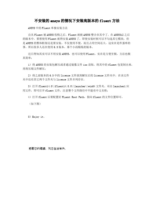
不安装的ansys的情况下安装高版本的fluent方法
ANSYS中的Fluent单独安装方法
自从Fluent被ANSYS收购之后,Fluent就被ANSYS整合在其中了,在ANSYS12之后
的版本中,要想使用Fluent就得安装ANSYS了,即使安装时候可以不勾选其它模块,但
是ANSYS的整体框架还是要安装,不仅使用不便,而且占用空间还大,这实在是件蛋疼的事,所以很多人还在使用6.3版本,那个小而精炼的版本。
近日得知其实可以不用安装ANSYS,也可以使用Fluent,实在是方便至极,方法也极
其简单:
1)将ANSYS的安装包解压或者通过镜像文件iso读取,将其中的fluent包复制出来,再将压缩文件解压;
2)将之前版本的6.3中的license文件放到解压后的license文件夹中,在该文件
夹中还有其它两个文件夹与license文件并列存在,
3)打开fluent14.0\\fluent14.0.0\\launcher\\win64文件夹,双击launcher1应
用文件,即可打开fluent文件,注意整个文件路径中不能有中文名称;
4)打开fluent后要配置好FLuent Root Path,指向fluent的文件位置即可,
(如下图)
5)Enjoy it。
感谢您的阅读,祝您生活愉快。
Fluent教程学习教程
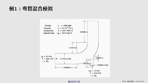
指定流体区域
第18页/共71页
第十八页,编辑于星期五:十九点 三十九分。
关闭DesignModeler
第19页/共71页
第十九页,编辑于星期五:十九点 三十九分。
第20页/共71页
第二十页,编辑于星期五:十九点 三十九分。
划分网格
第21页/共71页
第二十一页,编辑于星期五:十九点 三十九分 。
第34页/共71页
第三十四页,编辑于星期五:十九点 三十九分 。
第35页/共71页
第三十五页,编辑于星期五:十九点 三十九分 。
第36页/共71页
第三十六页,编辑于星期五:十九点 三十九分 。
启动Ansys Fluent
第37页/共71页
第三十七页,编辑于星期五:十九点 三十九分 。
第38页/共71页
第四十二页,编辑于星期五:十九点 三十九分 。
第43页/共71页
第四十三页,编辑于星期五:十九点 三十九分 。
第44页/共71页
第四十四页,编辑于星期五:十九点 三十九分 。
设置流体性质
第45页/共71页
第四十五页,编辑于星期五:十九点 三十九分 。
第46页/共71页
第四十六页,编辑于星期五:十九点 三十九分 。
第13页/共71页
第十三页,编辑于星期五:十九点 三十九分。
创建管道
第14页/共71页
第十四页,编辑于星期五:十九点 三十九分。
第15页/共71页
第十五页,编辑于星期五:十九点 三十九分。
第16页/共71页
第十六页,编辑于星期五:十九点 三十九分。
第17页/共71页
第十七页,编辑于星期五:十九点 三十九分。
第三十八页,编辑于星期五:十九点 三十九分 。
FLUENT13培训教材04求解器设置ANSYS公司
n启动 FMG 初始化
– 压力基求解器: /solve/init/fmg-initialization – 密度基求解器: 当选择密度基求解器后在 GUI里可见
nFMG 在粗网格上用多重网格求解
– 通过 TUI 命令来设置
/solve/init/set-fmg-initialization
PPT文档演模板
PPT文档演模板
FLUENT13培训教材04求解器设置 ANSYS公司
求解过程概览
n 求解参数 – 选择求解器 – 离散格式
n 初始条件 n 收敛
– 监测收敛过程 – 稳定性
• 设置松弛因子 • 设置 Courant number – 加速收敛 n 精度 – 网格无关性 – 自适应网格
PPT文档演模板
n对密度基求解器,即使稳态问题, 也存在瞬态项
– 用Courant 定义时间步长
n对显式求解器:
– 稳定性约束限制了最大Courant 数
• 不能超过 2 (缺省为1)
• 有收敛困难时减少 Courant 数
n对隐式求解器:
– Courant 没有稳定性约束限制
• 缺省值为 5.
PPT文档演模板
FLUENT13培训教材04求解器设置 ANSYS公司
加速收敛
n可以通过以下方法加速收敛:
– 设置更好的初场
• 从前次的计算结果开始(如需要,可以使用file/interpolation)
– 渐次增加松弛因子或Courant数
• 过高的值容易引起发散 • 继续迭代是应保存case和date文件
n 隐式方法一般优于显式,因为其对时间步有严格的限制 n 显式方法一般用于流动时间尺度和声学时间尺度相当的情况(如高马赫
- 1、下载文档前请自行甄别文档内容的完整性,平台不提供额外的编辑、内容补充、找答案等附加服务。
- 2、"仅部分预览"的文档,不可在线预览部分如存在完整性等问题,可反馈申请退款(可完整预览的文档不适用该条件!)。
- 3、如文档侵犯您的权益,请联系客服反馈,我们会尽快为您处理(人工客服工作时间:9:00-18:30)。
Ansys FLUENT Tutorials└─ANSYS FLUENT├─ANSYS-FLUENT-Intro_13.0_1st-ed_pdf││fluent_13.0_Agenda.pdf││fluent_13.0_TOC.pdf│││├─lectures││fluent_13.0_lecture01-welcome.pdf││fluent_13.0_lecture02-intro-to-cfd.pdf││fluent_13.0_lecture03-solver-basics.pdf││fluent_13.0_lecture04-boundary-conditions.pdf ││fluent_13.0_lecture05-solver-settings.pdf││fluent_13.0_lecture06-turbulence.pdf││fluent_13.0_lecture07-heat-transfer.pdf││fluent_13.0_lecture08-udf.pdf││fluent_13.0_lecture09-physics.pdf││fluent_13.0_lecture10-transient.pdf││fluent_13.0_lecture11-post.pdf│││├─workshop-input-files││├─workshop1-mixing-tee│││ fluidtee.meshdat│││││├─workshop2-airfoil-new│││ NACA0012.msh│││ mach_0.5_comparison.cas.gz│││ mach_0.5_comparison.dat.gz│││ mach_0.7_converged.cas.gz│││ mach_0.7_converged.dat.gz│││ test-data-bottom.xy│││ test-data-top.xy│││││├─workshop3-multi-species│││ calc_activities.jou│││ garage.msh│││ workshop3-converged.cas.gz│││ workshop3-converged.dat.gz│││││├─workshop4-electronics│││ heatsink.msh.gz│││ ws4_no-radiation.cas.gz│││ ws4_no-radiation.dat.gz│││ ws4_s2s-radiation.cas.gz│││ ws4_s2s-radiation.dat.gz│││ ws4_viewfactor.s2s.gz│││││├─workshop5-moving-parts│││ ws5-mesh-animation.avi│││ ws5-simple-wind-turbine.msh│││ ws5_udf_for_motion.c│││││├─workshop6-dpm│││ dpm_tutorial.msh│││││└─workshop7-tank-flush││tankflush.msh.gz││ws7-tankflush-animation.avi││ws7-tankflush-animation.mpeg│││└─workshops│fluent_13.0_WS_TOC.pdf│fluent_13.0_workshop01-mixingtee.pdf│fluent_13.0_workshop02-airfoil.pdf│fluent_13.0_workshop03-Multiple-Species.pdf│fluent_13.0_workshop04-electronics.pdf│fluent_13.0_workshop05-moving-parts.pdf│fluent_13.0_workshop06-dpm.pdf│fluent_13.0_workshop07-tank-flush.pdf│├─Quick Tutorials││ FLUENT_Overview_1_Introduction_to_FLUENT12_in_ANSYS_Workbench_DOC.pd f││ FLUENT_Overview_1_Introduction_to_FLUENT12_in_ANSYS_Workbench_WA TCH ME.swf││ FLUENT_Overview_2_Creating_and_Comparing_Related_FLUENT12_Analyses_in_ ANSYS_Workbench_DOC.pdf││ FLUENT_Overview_2_Creating_and_Comparing_Related_FLUENT12_Analyses_in_ ANSYS_Workbench_WA TCHME.swf││ FLUENT_Overview_3_Parametric_Study_Using_FLUENT12_in_ANSYS_Workbench _DOC.pdf││ FLUENT_Overview_3_Parametric_Study_Using_FLUENT12_in_ANSYS_Workbench _WATCHME.swf││ FLUENT_Overview_4_1-Way_Fluid-Structure_Interaction_Using_FLUENT12_and_A NSYS_Mechanical_DOC.pdf││ FLUENT_Overview_4_1-Way_Fluid-Structure_Interaction_Using_FLUENT12_and_A NSYS_Mechanical_WA TCHME.swf│││├─FLUENT_Overview_1_FILES││ probe.agdb│││├─FLUENT_Overview_2_FILES│││ Duplicate_Probe_Fluent.wbpj│││││└─Duplicate_Probe_Fluent_files│││ .project_cache│││││├─dp0││││ designPoint.wbdp│││││││├─FFF││││├─DM│││││ FFF.agdb│││││││││├─Fluent│││││ FFF-1-00100.dat.gz│││││ FFF-1.cas.gz│││││ FFF.set│││││││││├─MECH│││││ FFF.msh│││││││││└─Post││││Probe.cst│││││││├─FFF-1││││└─Fluent││││FFF-1.1-1-00081.dat.gz │││││││└─global│││└─MECH││││ FFF.mshdb│││││││└─FFF││└─user_files│├─FLUENT_Overview_3_FILES│││ Parametric_Probe_Fluent.wbpj│││││└─Parametric_Probe_Fluent_files│││ .project_cache│││││├─dp0││││ designPoint.wbdp│││││││├─FFF││││├─DM│││││ FFF.agdb│││││││││├─Fluent│││││ FFF-1-00100.dat.gz│││││ FFF-1.cas.gz│││││ FFF.set│││││││││├─MECH│││││ FFF.msh│││││││││└─Post││││Probe.cst│││││││├─FFF-1││││└─Fluent││││FFF-1.1-1-00081.dat.gz │││││││└─global│││└─MECH││││ FFF.mshdb│││││││└─FFF││└─user_files│└─FLUENT_Overview_4_FILES││ FSI_Probe_Fluent.wbpj│││└─FSI_P robe_Fluent_files││ .project_cache│││├─dp0│││ designPoint.wbdp│││││├─FFF│││├─DM││││ FFF.agdb│││││││├─Fluent││││ FFF-1-00100.dat.gz││││ FFF-1.cas.gz││││ FFF.set│││││││├─MECH││││ FFF.msh│││││││└─Post│││Probe.cst│││││├─FFF-1│││└─Fluent│││FFF-1.1-1-00081.dat.gz│││││└─global││└─MECH│││ FFF.mshdb│││││└─FFF│└─user_files├─combustion-fluent││ combustion-tutorial-list_13.0.pdf││ tut-01-intro-tut-16-species-transport.pdf││ tut-02-intro-tut-17-non-premix-combustion.pdf ││ tut-03-intro-tut-18-surface-chemistry.pdf││ tut-04-intro-tut-19-evaporating-liquid.pdf││ tut-05-berl.pdf││ tut-06-finite-rate.pdf││ tut-07-pdf-jet.pdf││ tut-08-cijr.pdf││ tut-09-pilot-jet.pdf││ tut-10-zimont.pdf││ tut-11-surfchem.pdf││ tut-12-mchar.pdf││ tut-13-co-combustor.pdf││ tut-14-flamelet.pdf││ tut-15-moss-brookes.pdf││ tut-16-dqmom.pdf││ tut-17-species.pdf││ tut-18-euler-granular.pdf││ tut-19-dpm-channel.pdf│││├─tut-01-intro-tut-16-species-transport│││ gascomb.msh│││││└─solution_files││gascomb1.cas.gz││gascomb1.dat.gz││gascomb2.dat.gz││gascomb3.cas.gz││gascomb3.dat.gz│││├─tut-02-intro-tut-17-non-premix-combustion │││ berl.msh│││ berl.prof│││││└─solution_files││berl-1.cas.gz││berl-1.dat.gz││berl.pdf│││├─tut-03-intro-tut-18-surface-chemistry│││ surface.msh│││││└─solution_files││surface-non-react.cas.gz││surface-react1.cas.gz││surface-react1.dat.gz││surface-react2.cas.gz││surface-react2.dat.gz│││├─tut-04-intro-tut-19-evaporating-liquid│││ sector.msh│││││└─solution_files││sector.msh││spray1.cas.gz││spray1.dat.gz││spray2.cas.gz││spray2.dat.gz││spray3.cas.gz││spray3.dat.gz│││├─tut-05-berl│││ berl.msh.gz│││ berl.prof│││││└─solution_files││berl-mag-1.cas.gz││berl-mag-1.dat.gz││berl-mag-2.cas.gz││berl-mag-3.cas.gz ││berl-mag-3.dat.gz │││├─tut-06-finite-rate│││ conreac.msh.gz│││││└─solution_files││5step.cas.gz││5step.dat.gz││5step_cold.cas.gz ││5step_cold.dat.gz ││5step_final.cas.gz │││├─tut-07-pdf-jet│││ CH4-skel.che│││ flameD.msh.gz│││ therm.dat│││││└─solution_files││flameD-1.cas.gz ││flameD-1.dat.gz ││flameD-2.cas.gz ││flameD-2.dat.gz ││flameD-3.cas.gz ││flameD-3.dat.gz ││flameD.pdf.gz││surf-mon-1.out │││├─tut-08-cijr│││ CIJR-therm.dat│││ CIJR.che│││ CIJR.msh.gz│││││└─solution_files││CIJR-1.cas.gz││CIJR-1.dat.gz││CIJR-2.cas.gz││CIJR-2.dat.gz││CIJR-3.cas.gz││CIJR-3.dat.gz││CIJR-4.cas.gz││CIJR-4.dat.gz││CIJR-4.fla.gz││CIJR.fla.gz││CIJR.pdf.gz││CIJRdisplay.cas.gz ││CIJRdisplay.dat.gz │││├─tut-09-pilot-jet│││ flameD-sfla.msh.gz│││ gri30.che│││││└─solution_files││flameD-sfla-1.cas.gz ││flameD-sfla-1.dat.gz ││flameD-sfla.fla.gz ││flameD-sfla.pdf.gz ││flameD-ufla-1.cas.gz ││flameD-ufla-1.dat.gz ││flameD-ufla-1.fla.gz ││surf-mon-1.out│││├─tut-10-zimont│││ conreac.msh│││││└─solution_files││zimont-ad.cas.gz││zimont-ad.dat.gz││zimont-nonad.cas.gz ││zimont-nonad.dat.gz ││zimont.cas.gz│││├─tut-11-surfchem│││ gas_chem.che│││ surf_chem.che│││ test.msh.gz│││││└─solution_files││surf-cat-comb.cas.gz ││surf-cat-comb.dat.gz ││surf-mon-1.out│││├─tu t-12-mchar│││ mchar.msh.gz│││││└─solution_files││mchar-rad.cas.gz││mchar-rad.dat.gz││mchar.cas.gz││mchar.dat.gz││view-0.vw│││├─tut-13-co-combustor│││ par-premixed.msh.gz│││││└─solution_files││par-premixed.pdf.gz││peters-partially-premixed-2nd.cas.gz ││peters-partially-premixed-2nd.dat.gz ││zimont-partially-premixed-1st.cas.gz ││zimont-partially-premixed-1st.dat.gz ││zimont-partially-premixed-2nd.cas.gz ││zimont-partially-premixed-2nd.dat.gz ││zimont-partially-premixed.cas.gz││zimont-partially-premixed.dat.gz│││├─tut-14-flamelet│││ berl.msh.gz│││ berl.prof│││ smooke46.che│││ thermo.db│││││└─solution_files││berl-converged.cas.gz││berl-converged.dat.gz││berl-ini.cas.gz││berl-second.cas.gz││berl-second.dat.gz││berl.fla.gz││berl.pdf.gz│││├─tut-15-moss-brookes│││ brookes_ch4.cas.gz│││ brookes_ch4.dat.gz│││ brookes_ch4.pdf.gz│││ brookes_ch4.ray│││ flamlet.fla│││ therm.dat│││││└─solution_files││brookes_ch4_soot_converged.cas.gz││brookes_ch4_soot_converged.dat.gz │││├─tut-16-dqmom│││ dqmom.msh.gz│││││└─solution_files││dqmom-1.cas.gz││dqmom-1.dat.gz││dqmom-2.cas.gz││dqmom-2.dat.gz││dqmom-final.cas.gz││dqmom-final.dat.gz││dqmom-init.cas.gz││dqmom-init.dat.gz││dqmom.cas.gz││dqmom.dat.gz│││├─tut-17-species│││ baffled_reactor.msh.gz│││││└─solution_files││case-1-rtd-complete.cas.gz││case-1-rtd-complete.dat.gz││case-1-tracer-init.cas.gz││case-1-tracer-init.dat.gz││case-1-tracer-injection-complete.cas.gz ││case-1-tracer-injection-complete.dat.gz ││case-1-tracer.out││case-1.cas.gz││case-1.dat.gz││case-2-rtd-complete.cas.gz││case-2-rtd-complete.dat.gz││case-2-rtd-final.cas.gz││case-2-rtd-final.dat.gz││case-2-tracer-init.cas.gz││case-2-tracer-init.dat.gz││case-2-tracer-injection-complete.cas.gz ││case-2-tracer-injection-complete.dat.gz ││case-2-tracer.out││case-2.cas.gz││case-2.dat.gz││surf-mon-1.out│││├─tut-18-euler-granular│││ euler.msh.gz│││ mass_xfer_rate.c│││││└─solution_files││euler-gran-1.cas.gz││euler-gran-1.dat.gz││euler-gran-final.cas.gz││euler-gran-final.dat.gz││vol-solid.out│││└─tut-19-dpm-channel││ 3dpipe.msh.gz│││└─solution_files│ dpm-evap.cas.gz│ dpm-evap.dat.gz│ pipe-flow.cas.gz│ pipe-flow.dat.gz│├─extra││ FLUENT13_workshop_XX_RAE_Airfoil.pptx ││ FLUENT13_workshop_XX_V ortexShedding.pptx │││├─workshop_XX_RAE_Airfoil│││ ExperimentalData.csv│││ coarse.xy│││ experiment.xy│││ expressions.cst│││ rae2822_coarse.msh│││││└─Result_TUT_04│││ rae2822_coarse-data_export_to_post.cas │││ rae2822_coarse-data_export_to_post.cdat │││ rae2822_coarse-data_export_to_post.cst│││ rae2822_coarse.cas.gz│││ rae2822_coarse.dat.gz│││││└─FINE_MESH││ medium.xy││ rae2822_fine.cas.gz││ rae2822_fine.dat.gz││ rae2822_fine.msh││ rae2822_medium.cas.gz││ rae2822_medium.dat.gz││ rae2822_medium.msh│││└─workshop_XX_V ortexShedding││ point-4-y-velocity-final.out││ vortex-shedding-coarse.msh││ vortex-shedding-unsteady.cas.gz││ vortex-shedding-unsteady.dat.gz│││├─FILES_FOR_CFDPOST││ vectors.mp4││ vortex-shedding-unsteady-3-68.949997.dat.gz ││ vortex-shedding-unsteady-3-69.199997.dat.gz ││ vortex-shedding-unsteady-3-69.449997.dat.gz ││ vortex-shedding-unsteady-3-69.699997.dat.gz ││ vortex-shedding-unsteady-3-69.949997.dat.gz ││ vortex-shedding-unsteady-3-70.199997.dat.gz ││ vortex-shedding-unsteady-3-70.449997.dat.gz ││ vortex-shedding-unsteady-3-70.699997.dat.gz ││ vortex-shedding-unsteady-3-70.949997.dat.gz ││ vortex-shedding-unsteady-3-71.199997.dat.gz ││ vortex-shedding-unsteady-3-71.449997.dat.gz ││ vortex-shedding-unsteady-3-71.699997.dat.gz ││ vortex-shedding-unsteady-3-71.949997.dat.gz ││ vortex-shedding-unsteady-3-72.199997.dat.gz ││ vortex-shedding-unsteady-3-72.449997.dat.gz ││ vortex-shedding-unsteady-3-72.699997.dat.gz ││ vortex-shedding-unsteady-3-72.949997.dat.gz ││ vortex-shedding-unsteady-3-73.199997.dat.gz ││ vortex-shedding-unsteady-3-73.449997.dat.gz ││ vortex-shedding-unsteady-3-73.699997.dat.gz ││ vortex-shedding-unsteady-3-73.949997.dat.gz ││ vortex-shedding-unsteady-3-74.199997.dat.gz ││ vortex-shedding-unsteady-3-74.449997.dat.gz ││ vortex-shedding-unsteady-3-74.699997.dat.gz ││ vortex-shedding-unsteady-3-74.949997.dat.gz ││ vortex-shedding-unsteady-3-75.199997.dat.gz ││ vortex-shedding-unsteady-3-75.449997.dat.gz ││ vortex-shedding-unsteady-3-75.699997.dat.gz ││ vortex-shedding-unsteady-3-75.949997.dat.gz ││ vortex-shedding-unsteady-3-76.199997.dat.gz ││ vortex-shedding-unsteady-3-76.449997.dat.gz ││ vortex-shedding-unsteady-3-76.699997.dat.gz ││ vortex-shedding-unsteady-3-76.949997.dat.gz ││ vortex-shedding-unsteady-3-77.199997.dat.gz││ vortex-shedding-unsteady-3-77.699997.dat.gz ││ vortex-shedding-unsteady-3-77.949997.dat.gz ││ vortex-shedding-unsteady-3-78.199997.dat.gz ││ vortex-shedding-unsteady-3-78.449997.dat.gz ││ vortex-shedding-unsteady-3-78.699997.dat.gz ││ vortex-shedding-unsteady-3-78.949997.dat.gz ││ vortex-shedding-unsteady-3-79.199997.dat.gz ││ vortex-shedding-unsteady-3-79.449997.dat.gz ││ vortex-shedding-unsteady-3-79.699997.dat.gz ││ vortex-shedding-unsteady-3-79.949997.dat.gz ││ vortex-shedding-unsteady-3-80.199997.dat.gz ││ vortex-shedding-unsteady-3-80.449997.dat.gz ││ vortex-shedding-unsteady-3-80.699997.dat.gz ││ vortex-shedding-unsteady-3-80.950012.dat.gz ││ vortex-shedding-unsteady-3-81.200027.dat.gz ││ vortex-shedding-unsteady-3-81.450043.dat.gz ││ vortex-shedding-unsteady-3-81.700058.dat.gz ││ vortex-shedding-unsteady-3-81.950073.dat.gz ││ vortex-shedding-unsteady-3-82.200089.dat.gz ││ vortex-shedding-unsteady-3-82.450104.dat.gz ││ vortex-shedding-unsteady-3-82.700119.dat.gz ││ vortex-shedding-unsteady-3-82.950134.dat.gz ││ vortex-shedding-unsteady-3-83.200150.dat.gz ││ vortex-shedding-unsteady-3-83.450165.dat.gz ││ vortex-shedding-unsteady-3-83.700180.dat.gz ││ vortex-shedding-unsteady-3-83.950195.dat.gz ││ vortex-shedding-unsteady-3-84.200211.dat.gz ││ vortex-shedding-unsteady-3-84.450226.dat.gz ││ vortex-shedding-unsteady-3-84.700241.dat.gz ││ vortex-shedding-unsteady-3-84.950256.dat.gz ││ vortex-shedding-unsteady-3-85.200272.dat.gz ││ vortex-shedding-unsteady-3-85.450287.dat.gz ││ vortex-shedding-unsteady-3-85.700302.dat.gz ││ vortex-shedding-unsteady-3-85.950317.dat.gz ││ vortex-shedding-unsteady-3-86.200333.dat.gz ││ vortex-shedding-unsteady-3-86.450348.dat.gz ││ vortex-shedding-unsteady-3-86.700363.dat.gz ││ vortex-shedding-unsteady-3-86.950378.dat.gz ││ vortex-shedding-unsteady-3-87.200394.dat.gz ││ vortex-shedding-unsteady-3-87.450409.dat.gz ││ vortex-shedding-unsteady-3-87.700424.dat.gz ││ vortex-shedding-unsteady-3-87.950439.dat.gz ││ vortex-shedding-unsteady-3-88.200455.dat.gz││ vortex-shedding-unsteady-3-88.700485.dat.gz ││ vortex-shedding-unsteady-3-88.950500.dat.gz ││ vortex-shedding-unsteady-3-89.200516.dat.gz ││ vortex-shedding-unsteady-3-89.450531.dat.gz ││ vortex-shedding-unsteady-3-89.700546.dat.gz ││ vortex-shedding-unsteady-3-89.950562.dat.gz ││ vortex-shedding-unsteady-3-90.200577.dat.gz ││ vortex-shedding-unsteady-3-90.450592.dat.gz ││ vortex-shedding-unsteady-3-90.700607.dat.gz ││ vortex-shedding-unsteady-3-90.950623.dat.gz ││ vortex-shedding-unsteady-3-91.200638.dat.gz ││ vortex-shedding-unsteady-3-91.450653.dat.gz ││ vortex-shedding-unsteady-3-91.700668.dat.gz ││ vortex-shedding-unsteady-3-91.950684.dat.gz ││ vortex-shedding-unsteady-3-92.200699.dat.gz ││ vortex-shedding-unsteady-3-92.450714.dat.gz ││ vortex-shedding-unsteady-3-92.700729.dat.gz ││ vortex-shedding-unsteady-3.cas.gz│││└─Result-TUT_07││ cfd_post.cst││ point-4-y-velocity-final.out││ point-4-y-velocity.out││ sequence-1.mpeg││ vectors.mp4││ vortex-shedding-coarse-steady.cas.gz││ vortex-shedding-coarse-steady.dat.gz││ vortex-shedding-unsteady-final.cas.gz││ vortex-shedding-unsteady-final.dat.gz││ vortex-shedding-unsteady.cas.gz││ vortex-shedding-unsteady.dat.gz│││├─ADDITIONAL-FILES││ q-criterion2D.scm││ velocity.fft│││└─ANIMATION-FILES│ sequence-1.cxa│ sequence-1.mpeg│ sequence-1_0000.hmf│ sequence-1_0001.hmf│ sequence-1_0002.hmf│ sequence-1_0003.hmf│ sequence-1_0005.hmf │ sequence-1_0006.hmf │ sequence-1_0007.hmf │ sequence-1_0008.hmf │ sequence-1_0009.hmf │ sequence-1_0010.hmf │ sequence-1_0011.hmf │ sequence-1_0012.hmf │ sequence-1_0013.hmf │ sequence-1_0014.hmf │ sequence-1_0015.hmf │ sequence-1_0016.hmf │ sequence-1_0017.hmf │ sequence-1_0018.hmf │ sequence-1_0019.hmf │ sequence-1_0020.hmf │ sequence-1_0021.hmf │ sequence-1_0022.hmf │ sequence-1_0023.hmf │ sequence-1_0024.hmf │ sequence-1_0025.hmf │ sequence-1_0026.hmf │ sequence-1_0027.hmf │ sequence-1_0028.hmf │ sequence-1_0029.hmf │ sequence-1_0030.hmf │ sequence-1_0031.hmf │ sequence-1_0032.hmf │ sequence-1_0033.hmf │ sequence-1_0034.hmf │ sequence-1_0035.hmf │ sequence-1_0036.hmf │ sequence-1_0037.hmf │ sequence-1_0038.hmf │ sequence-1_0039.hmf │ sequence-1_0040.hmf │ sequence-1_0041.hmf │ sequence-1_0042.hmf │ sequence-1_0043.hmf │ sequence-1_0044.hmf │ sequence-1_0045.hmf │ sequence-1_0046.hmf │ sequence-1_0047.hmf│ sequence-1_0049.hmf │ sequence-1_0050.hmf │ sequence-1_0051.hmf │ sequence-1_0052.hmf │ sequence-1_0053.hmf │ sequence-1_0054.hmf │ sequence-1_0055.hmf │ sequence-1_0056.hmf │ sequence-1_0057.hmf │ sequence-1_0058.hmf │ sequence-1_0059.hmf │ sequence-1_0060.hmf │ sequence-1_0061.hmf │ sequence-1_0062.hmf │ sequence-1_0063.hmf │ sequence-1_0064.hmf │ sequence-1_0065.hmf │ sequence-1_0066.hmf │ sequence-1_0067.hmf │ sequence-1_0068.hmf │ sequence-1_0069.hmf │ sequence-1_0070.hmf │ sequence-1_0071.hmf │ sequence-1_0072.hmf │ sequence-1_0073.hmf │ sequence-1_0074.hmf │ sequence-1_0075.hmf │ sequence-1_0076.hmf │ sequence-1_0077.hmf │ sequence-1_0078.hmf │ sequence-1_0079.hmf │ sequence-1_0080.hmf │ sequence-1_0081.hmf │ sequence-1_0082.hmf │ sequence-1_0083.hmf │ sequence-1_0084.hmf │ sequence-1_0085.hmf │ sequence-1_0086.hmf │ sequence-1_0087.hmf │ sequence-1_0088.hmf │ sequence-1_0089.hmf │ sequence-1_0090.hmf │ sequence-1_0091.hmf│ sequence-1_0093.hmf│ sequence-1_0094.hmf│ sequence-1_0095.hmf│ sequence-1_0096.hmf│ sequence-1_0097.hmf│ sequence-1_0098.hmf│ sequence-1_0099.hmf│ sequence-1_0100.hmf│ sequence-1_0101.hmf│ sequence-1_0102.hmf│ sequence-1_0103.hmf│ sequence-1_0104.hmf│ sequence-1_0105.hmf│ sequence-1_0106.hmf│ sequence-1_0107.hmf│ sequence-1_0108.hmf│ sequence-1_0109.hmf│ sequence-1_0110.hmf│ sequence-1_0111.hmf│ sequence-1_0112.hmf│ sequence-1_0113.hmf│ sequence-1_0114.hmf│ sequence-1_0115.hmf│ sequence-1_0116.hmf│ sequence-1_0117.hmf│ sequence-1_0118.hmf│ sequence-1_0119.hmf│├─fluent-heat-transfer││ ht-01-intro-tut-04-periodic-flow-heat.pdf││ ht-02-intro-tut-07-radiation-and-convection.pdf ││ ht-03-intro-tut-08-DO-radiation.pdf││ ht-04-intro-tut-24-solidification.pdf││ ht-05-conjugate-heat-transfer.pdf││ ht-06-compact-heat-exchanger.pdf││ ht-07-macro-heat-exchanger.pdf││ ht-08-head-lamp.pdf│││├─ht-01-intro-tut-04-periodic-flow-heat│││ tubebank.msh│││││└─solution_files││tubebank.cas.gz││tubebank.dat.gz│││├─ht-02-intro-tut-07-radiation-and-convection │││ rad.msh.gz│││││└─solution_files││rad_1.s2s.gz││rad_10.cas.gz││rad_10.dat.gz││rad_10.s2s.gz││rad_100.cas.gz││rad_100.dat.gz││rad_100.s2s.gz││rad_1600.cas.gz││rad_1600.dat.gz││rad_1600.s2s.gz││rad_400.cas.gz││rad_400.dat.gz││rad_400.s2s.gz││rad_800.cas.gz││rad_800.dat.gz││rad_800.s2s.gz││rad_a_1.cas.gz││rad_b_1.cas.gz││rad_b_1.dat.gz││rad_partial.cas.gz││rad_partial.dat.gz││rad_partial.s2s.gz││tp_1.xy││tp_10.xy││tp_100.xy││tp_1600.xy││tp_400.xy││tp_800.xy││tp_partial.xy│││├─ht-03-intro-tut-08-DO-radiation│││ do.msh.gz│││││└─solution_files││do.cas.gz││do.dat.gz││do_2x2_10x10_pix.cas.gz││do_2x2_10x10_pix.dat.gz││do_2x2_1x1.xy││do_2x2_2x2_pix.cas.gz││do_2x2_2x2_pix.dat.gz││do_2x2_2x2_pix.xy││do_2x2_3x3_div.cas.gz││do_2x2_3x3_div.dat.gz││do_2x2_3x3_div.xy││do_2x2_3x3_pix.cas.gz││do_2x2_3x3_pix.dat.gz││do_2x2_3x3_pix.xy││do_3x3_3x3_div.cas.gz││do_3x3_3x3_div.dat.gz││do_3x3_3x3_div.xy││do_3x3_3x3_div_baf_int.xy ││do_3x3_3x3_div_df1.cas.gz ││do_3x3_3x3_div_df1.dat.gz ││do_3x3_3x3_div_df=1.xy ││do_3x3_3x3_div_int.cas.gz ││do_3x3_3x3_div_int.dat.gz ││do_5x5_3x3_div.cas.gz││do_5x5_3x3_div.dat.gz││do_5x5_3x3_div.xy│││├─ht-04-intro-tut-24-solidification│││ solid.msh│││││└─solution_files││solid.cas.gz││solid.dat.gz││solid0.cas.gz││solid0.dat.gz││solid01.cas.gz││solid01.dat.gz││solid5.cas.gz││solid5.dat.gz│││├─ht-05-conjugate-heat-transfer│││ chip3d.msh.gz│││││└─solution_files││chip3d-adapt1.cas.gz││chip3d-adapt1.dat.gz││chip3d-adapt2.cas.gz││chip3d.cas.gz││chip3d.dat.gz││surf-mon-1.out││temp-0.xy││temp-1.xy││temp-2.xy││velocity-0.xy││velocity-1.xy││velocity-2.xy││xwss-0.xy││xwss-1.xy││xwss-2.xy│││├─ht-06-compact-heat-exchanger │││ htx.msh.gz│││││└─solution_files││htx-energy.cas.gz││htx-energy.dat.gz││htx-eqn.cas.gz││htx-eqn.dat.gz││htx-final.cas.gz││htx-final.dat.gz││htx-setup.cas.gz││htx-setup.dat.gz││surf-mon-1.out│││├─ht-07-macro-heat-exchanger │││ rad.tab│││ wedge.msh.gz│││││└─solution_files││wedge1.cas.gz││wedge1.dat.gz││wedge2.cas.gz││wedge2.dat.gz││wedge3.cas.gz││wedge3.dat.gz││wedge4.cas.gz││wedge4.dat.gz│││└─ht-08-head-lamp││ head-lamp.msh.gz│││└─solution_fi les│ auto-hlamp.cas.gz│ auto-hlamp.dat.gz│ head-lamp-t.out│ hed-lamp-v.out│├─multiphase-fluent││ 01-hfilm.pdf││ 02-boil.pdf││ 03-nucleate_boil.pdf││ 04-dambreak.pdf││ 05-sloshing.pdf││ 06-bubble-col.pdf││ 07-bubble-break.pdf││ 08-inkjet.pdf││ 09-sparger.pdf││ 10-pbed-reactor.pdf││ 11-ddpm.pdf││ 12-dm-ship-wave.pdf││ 13-udf-clarifier.pdf││ 14-udf-fbed.pdf│││├─tut-01-hfilm│││ boiling.c│││ test-2d.msh.gz│││││└─solution_files│││ hfilm_input_files.tar.zg │││ nusselt-1.out│││ test-2d-1-00100.dat│││ test-2d-1-00200.dat│││ test-2d-1-00300.dat│││ test-2d-1-00400.dat│││ test-2d-1-00500.dat│││ test-2d-1-00600.dat│││ test-2d-1-00700.dat│││ test-2d-1-00800.dat│││ test-2d-1-00900.dat│││ test-2d-1-01000.dat│││ test-2d-1-01100.dat│││ test-2d-1-01200.dat│││ test-2d-1-01300.dat│││ test-2d-1-01400.dat│││ test-2d-1-01500.dat│││ test-2d-1-01600.dat│││ test-2d-1-01700.dat│││ test-2d-1-01800.dat│││ test-2d-1-01900.dat│││ test-2d-1-02000.dat│││ test-2d-1-02100.dat│││ test-2d-1-02200.dat│││ test-2d-1-02300.dat│││ test-2d-1-02400.dat│││ test-2d-1-02500.dat│││ test-2d-1-02600.dat│││ test-2d-1-02700.dat│││ test-2d-1-02800.dat│││ test-2d-1-02900.dat│││ test-2d-1-03000.dat│││ test-2d-1-03100.dat│││ test-2d-1-03200.dat│││ test-2d-1-03300.dat│││ test-2d-1-03400.dat│││ test-2d-1-03500.dat│││ test-2d-1-03600.dat│││ test-2d-1-03700.dat│││ test-2d-1-03800.dat│││ test-2d-1-03900.dat│││ test-2d-1-04000.dat│││ test-2d-1.cas│││ vol-mon-1.out│││││└─libudf││├─ntx86│││└─2ddp│││boiling.obj│││libudf.dll│││libudf.exp│││libudf.lib│││log│││makefile│││udf_names.c │││udf_names.obj │││user_nt.udf│││││├─src│││ boiling.c│││││└─win64││└─2ddp││boiling.obj││libudf.dll││libudf.exp││libudf.lib││log││makefile││ud_io1.h││udf_names.c ││udf_names.obj ││user_nt.udf│││├─tut-02-boil│││ boil.msh.gz│││││└─solution_files││boil-3-00300.dat.gz││boil-3-01000.dat.gz││boil-3.cas.gz│││├─tut-03-nucleate-boil│││ boiling-conjugate.msh│││││└─solution_files││boil-final.cas.gz││boil-final.dat.gz││boil-init.cas.gz││boil-init.dat.gz││boil-single-phase.cas.gz ││boil-single-phase.dat.gz ││liquid-outlet.prof││surf-mon-1.out││surf-mon-2.out│││├─tut-04-dambreak│││ dambreak.msh.gz│││││└─solution_files││dambreak-100.cas.gz││dambreak-100.dat.gz││dambreak-50.cas.gz││dambreak-50.dat.gz││dambreak-80.cas.gz││dambreak-80.dat.gz││dambreak.cas.gz││dambreak.dat.gz│││├─tut-05-sloshing│││ ft11.msh.gz│││││└─solution_files││├─baffles│││ baffles-data-file-4-02060.dat.gz │││ baffles-data-file-4-02080.dat.gz │││ baffles-images.zip│││ baffles.jou│││ ft11.msh.gz│││ operating.cas.gz│││ t=0.0s.cas.gz│││ t=0.0s.dat.gz│││ t=0.45s.cas.gz│││ t=0.45s.dat.gz│││ t=1.25s.cas.gz│││ t=1.25s.dat.gz│││ t=1.50s.cas.gz│││ t=1.50s.dat.gz│││ t=1.5s.cas.gz│││ t=1.5s.dat.gz│││ t=2.5s.cas.gz│││ t=2.5s.dat.gz│││││└─no-baffles││ no-baffles-data-file-4-02760.dat.gz ││ no-baffles-data-file-4-02780.dat.gz ││ no-baffles-images.zip││ no-baffles.jou││ t=0.0s.cas.gz││ t=0.0s.dat.gz││ t=0.45s.cas.gz││ t=0.45s.dat.gz││ t=0s.cas.gz││ t=0s.dat.gz││ t=1.25s.cas.gz││ t=1.25s.dat.gz││ t=1.5s.cas.gz││ t=1.5s.dat.gz││ t=2.5s.cas.gz││ t=2.5s.dat.gz││ tiff-no-baffles.zip │││├─tut-06-bubble-col│││ becker.msh│││││└─solution_files││becker-1-00200.dat.gz ││becker-1-00400.dat.gz ││becker-1-00600.dat.gz ││becker-1-00800.dat.gz ││becker-1-01000.dat.gz ││becker-1-01200.dat.gz ││becker-1-01400.dat.gz ││becker-1-01600.dat.gz ││becker-1-01800.dat.gz ││becker-1-02000.dat.gz ││becker-1-02200.dat.gz ││becker-1-02400.dat.gz ││becker-1-02600.dat.gz ││becker-1-02800.dat.gz ││becker-1-03000.dat.gz ││becker-1-03200.dat.gz ││becker-1-03400.dat.gz ││becker-1-03600.dat.gz ││becker-1-03800.dat.gz ││becker-1-04000.dat.gz ││becker-1-04200.dat.gz ││becker-1-04400.dat.gz ││becker-1-04600.dat.gz ││becker-1-04800.dat.gz ││becker-1-05000.dat.gz ││becker-1.cas.gz││becker.cas.gz││becker.dat.gz││vel-vectors.cxa││vel-vectors_0000.hmf ││vel-vectors_0001.hmf ││vel-vectors_0002.hmf ││vel-vectors_0003.hmf ││vel-vectors_0004.hmf ││vel-vectors_0005.hmf ││vel-vectors_0006.hmf││vel-vectors_0007.hmf ││vel-vectors_0008.hmf ││vel-vectors_0009.hmf ││vel-vectors_0010.hmf ││vel-vectors_0011.hmf ││vel-vectors_0012.hmf ││vel-vectors_0013.hmf ││vel-vectors_0014.hmf ││vel-vectors_0015.hmf ││vel-vectors_0016.hmf ││vel-vectors_0017.hmf ││vel-vectors_0018.hmf ││vel-vectors_0019.hmf ││vel-vectors_0020.hmf ││vel-vectors_0021.hmf ││vel-vectors_0022.hmf ││vel-vectors_0023.hmf ││vel-vectors_0024.hmf ││vof.cxa││vof_0000.hmf││vof_0001.hmf││vof_0002.hmf││vof_0003.hmf││vof_0004.hmf││vof_0005.hmf││vof_0006.hmf││vof_0007.hmf││vof_0008.hmf││vof_0009.hmf││vof_0010.hmf││vof_0011.hmf││vof_0012.hmf││vof_0013.hmf││vof_0014.hmf││vof_0015.hmf││vof_0016.hmf││vof_0017.hmf││vof_0018.hmf││vof_0019.hmf││vof_0020.hmf││vof_0021.hmf││vof_0022.hmf││vof_0023.hmf││vof_0024.hmf│││├─tut-07-bubble-break│││ bubcol_new2.msh.gz│││││└─solution_files││bubcol-final.cas.gz││bubcol-final.dat.gz││bubcol_new2-initial.cas.gz ││bubcol_new2-initial.dat.gz ││surf-mon-1.out││surf-mon-2.out││surf-mon-3.out│││├─tut-08-inkjet│││ inkjet.msh.gz│││ inlet1.c│││ udfconfig.h│││││└─solution_files││inkjet-1-00100.dat.gz││inkjet-1-00200.dat.gz││inkjet-1-00300.dat.gz││inkjet-1-00400.dat.gz││inkjet-1-00500.dat.gz││inkjet-1-00600.dat.gz││inkjet-1-00700.dat.gz││inkjet-1-00800.dat.gz││inkjet-1-00900.dat.gz││inkjet-1-01000.dat.gz││inkjet-1-01100.dat.gz││inkjet-1-01200.dat.gz││inkjet-1-01300.dat.gz││inkjet-1-01400.dat.gz││inkjet-1-01500.dat.gz││inkjet-1.cas.gz││inkjet-final.cas.gz││inkjet-final.dat.gz││inkjet.cas.gz││inkjet.dat.gz│││├─tut-09-sparger│││ sparger.msh.gz│││││└─solution_files。