克鲁格曼《国际经济学》(国际金融)习题答案要点
克鲁格曼《国际经济学》计算题及标准答案
1. 在古典贸易模型中,假设A 国有120名劳动力,B 国有50名劳动力,如果生产棉花的话,A 国的人均产量是2吨,B 国也是2吨;要是生产大米的话,A 国的人均产量是10吨,B 国则是16吨。
画出两国的生产可能性曲线并分析两国中哪一国拥有生产大米的绝对优势?哪一国拥有生产大米的比较优势?思路:B 国由于每人能生产16吨大米,而A 国每人仅生产10吨大米,所以B 国具有生产大米的绝对优势。
从两国生产可能性曲线看出A 国生产大米的机会成本为0.2,而B 国为0.125,所以B国生产大米的机会成本或相对成本低于A 国,B国生产大米具有比较优势。
2.下表列出了加拿大和中国生产1单位计算机和1单位小麦所需的劳动时间。
假定生产计算机和小麦都只用劳动,加拿大的总劳动为600小时,中国总劳动为800小时。
(1) 计算不发生贸易时各国生产计算机和小麦的产量。
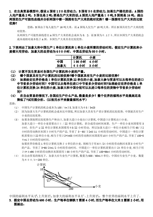
(2) 哪个国家具有生产计算机的比较优势?哪个国家具有生产小麦的比较优势?(3) 如果给定世界价格是1单位计算机交换22单位的小麦,加拿大参与贸易可以从每单位的进口中节省多少劳动时间?中国可以从每单位进口中节省多少劳动时间?如果给定世界价格是1单位计算机交换24单位的小麦,加拿大和中国分别可以从进口每单位的货物中节省多少劳动时间?(4) 在自由贸易的情况下,各国应生产什么产品,数量是多少?整个世界的福利水平是提高还是降低了?试用图分析。
(以效用水平来衡量福利水平)思路:(1) 中国生产计算机的机会成本为100/4=25,加拿大为60/3=20(2) 因为加拿大生产计算机的机会成本比中国低,所以加拿大具有生产者计算机的比较优势,中国就具有生产小麦的比较优势。
(3) 如果各国按照比较优势生产和出口,加拿大进口小麦出口计算机,中国进口计算机出口小麦。
加拿大进口一单位小麦需要出口1/22单位计算机,折合成劳动时间来算,生产一单位小麦本国要用3小时,但生产1/22单位计算机本国要用60/22小时劳动,所以加拿大进口一单位小麦相当于用60/22小时的劳动换回本国3小时生产的产品,节省了3-60/22=3/11小时的劳动时间。
国际经济学克鲁格曼课后习题答案章完整版

国际经济学克鲁格曼课后习题答案章集团标准化办公室:[VV986T-J682P28-JP266L8-68PNN]第一章练习与答案1.为什么说在决定生产和消费时,相对价格比绝对价格更重要?答案提示:当生产处于生产边界线上,资源则得到了充分利用,这时,要想增加某一产品的生产,必须降低另一产品的生产,也就是说,增加某一产品的生产是有机会机本(或社会成本)的。
生产可能性边界上任何一点都表示生产效率和充分就业得以实现,但究竟选择哪一点,则还要看两个商品的相对价格,即它们在市场上的交换比率。
相对价格等于机会成本时,生产点在生产可能性边界上的位置也就确定了。
所以,在决定生产和消费时,相对价格比绝对价格更重要。
2.仿效图1—6和图1—7,试推导出Y商品的国民供给曲线和国民需求曲线。
答案提示:3.在只有两种商品的情况下,当一个商品达到均衡时,另外一个商品是否也同时达到均衡?试解释原因。
答案提示:4.如果生产可能性边界是一条直线,试确定过剩供给(或需求)曲线。
答案提示:5.如果改用Y商品的过剩供给曲线(B国)和过剩需求曲线(A国)来确定国际均衡价格,那么所得出的结果与图1—13中的结果是否一致?6.答案提示:国际均衡价格将依旧处于贸易前两国相对价格的中间某点。
7.说明贸易条件变化如何影响国际贸易利益在两国间的分配。
答案提示:一国出口产品价格的相对上升意味着此国可以用较少的出口换得较多的进口产品,有利于此国贸易利益的获得,不过,出口价格上升将不利于出口数量的增加,有损于出口国的贸易利益;与此类似,出口商品价格的下降有利于出口商品数量的增加,但是这意味着此国用较多的出口换得较少的进口产品。
对于进口国来讲,贸易条件变化对国际贸易利益的影响是相反的。
8.如果国际贸易发生在一个大国和一个小国之间,那么贸易后,国际相对价格更接近于哪一个国家在封闭下的相对价格水平?答案提示:贸易后,国际相对价格将更接近于大国在封闭下的相对价格水平。
克鲁格曼《国际经济学》(国际金融部分)课后习题答案(英文版)第一章
克鲁格曼《国际经济学》(国际金融部分)课后习题答案(英文版)第一章CHAPTER 1INTRODUCTIONChapter OrganizationWhat is International Economics About?The Gains from TradeThe Pattern of TradeProtectionismThe Balance of PaymentsExchange-Rate DeterminationInternational Policy CoordinationThe International Capital MarketInternational Economics: Trade and MoneyCHAPTER OVERVIEWThe intent of this chapter is to provide both an overview of the subject matter of international economics and to provide a guide to the organization of the text. It is relatively easy for an instructor to motivate the study of international trade and finance. The front pages of newspapers, the covers of magazines, and the lead reports of television news broadcasts herald the interdependence of the U.S. economy with the rest of the world. This interdependence may also be recognized by students through their purchases of imports of all sorts of goods, their personal observations of the effects of dislocations due to international competition, and their experience through travel abroad.The study of the theory of international economics generates an understanding of many key events that shape our domesticand international environment. In recent history, these events include the causes and consequences of the large current account deficits of the United States; the dramatic appreciation of the dollar during the first half of the 1980s followed by its rapid depreciation in the second half of the 1980s; the Latin American debt crisis of the 1980s and the Mexico crisis in late 1994; and the increased pressures for industry protection against foreign competition broadly voiced in the late 1980s and more vocally espoused in the first half of the 1990s. Most recently, the financial crisis that began in East Asia in 1997 andspread to many countries around the globe and the Economic and Monetary Union in Europe have highlighted the way in which various national economies are linked and how important it is for us to understand these connections. At the same time, protests at global economic meetings have highlighted opposition to globalization. The text material will enable students to understand the economic context in which such events occur.Chapter 1 of the text presents data demonstrating the growth in trade and increasing importance of international economics. This chapter also highlights and briefly discusses seven themes which arise throughout the book. These themes include: 1) the gains from trade;2) the pattern of trade; 3) protectionism; 4), the balance of payments; 5) exchange rate determination; 6) international policy coordination; and 7) the international capital market. Students will recognize that many of the central policy debates occurring today come under the rubric of one of these themes. Indeed, it is often a fruitful heuristic to use current events to illustrate the force of the key themes and arguments which are presentedthroughout the text.。
克鲁格曼《国际经济学》(国际金融)习题标准答案要点

克鲁格曼《国际经济学》(国际金融)习题答案要点————————————————————————————————作者:————————————————————————————————日期:23 《国际经济学》(国际金融)习题答案要点第12章 国民收入核算与国际收支1、如问题所述,GNP 仅仅包括最终产品和服务的价值是为了避免重复计算的问题。
在国民收入账户中,如果进口的中间品价值从GNP 中减去,出口的中间品价值加到GNP 中,重复计算的问题将不会发生。
例如:美国分别销售钢材给日本的丰田公司和美国的通用汽车公司。
其中出售给通用公司的钢材,作为中间品其价值不被计算到美国的GNP 中。
出售给日本丰田公司的钢材,钢材价值通过丰田公司进入日本的GNP ,而最终没有进入美国的国民收入账户。
所以这部分由美国生产要素创造的中间品价值应该从日本的GNP 中减去,并加入美国的GNP 。
2、(1)等式12-2可以写成()()p CA S I T G =-+-。
美国更高的进口壁垒对私人储蓄、投资和政府赤字有比较小或没有影响。
(2)既然强制性的关税和配额对这些变量没有影响,所以贸易壁垒不能减少经常账户赤字。
不同情况对经常账户产生不同的影响。
例如,关税保护能提高被保护行业的投资,从而使经常账户恶化。
(当然,使幼稚产业有一个设备现代化机会的关税保护是合理的。
)同时,当对投资中间品实行关税保护时,由于受保护行业成本的提高可能使该行业投资下降,从而改善经常项目。
一般地,永久性和临时性的关税保护有不同的效果。
这个问题的要点是:政策影响经常账户方式需要进行一般均衡、宏观分析。
3、(1)、购买德国股票反映在美国金融项目的借方。
相应地,当美国人通过他的瑞士银行账户用支票支付时,因为他对瑞士请求权减少,故记入美国金融项目的贷方。
这是美国用一个外国资产交易另外一种外国资产的案例。
(2)、同样,购买德国股票反映在美国金融项目的借方。
当德国销售商将美国支票存入德国银行并且银行将这笔资金贷给德国进口商(此时,记入美国经常项目的贷方)或贷给个人或公司购买美国资产(此时,记入美国金融项目的贷方)。
克鲁格曼《国际经济学》(国际金融)习题标准答案要点
克鲁格曼《国际经济学》(国际金融)习题答案要点————————————————————————————————作者:————————————————————————————————日期:23 《国际经济学》(国际金融)习题答案要点第12章 国民收入核算与国际收支1、如问题所述,GNP 仅仅包括最终产品和服务的价值是为了避免重复计算的问题。
在国民收入账户中,如果进口的中间品价值从GNP 中减去,出口的中间品价值加到GNP 中,重复计算的问题将不会发生。
例如:美国分别销售钢材给日本的丰田公司和美国的通用汽车公司。
其中出售给通用公司的钢材,作为中间品其价值不被计算到美国的GNP 中。
出售给日本丰田公司的钢材,钢材价值通过丰田公司进入日本的GNP ,而最终没有进入美国的国民收入账户。
所以这部分由美国生产要素创造的中间品价值应该从日本的GNP 中减去,并加入美国的GNP 。
2、(1)等式12-2可以写成()()p CA S I T G =-+-。
美国更高的进口壁垒对私人储蓄、投资和政府赤字有比较小或没有影响。
(2)既然强制性的关税和配额对这些变量没有影响,所以贸易壁垒不能减少经常账户赤字。
不同情况对经常账户产生不同的影响。
例如,关税保护能提高被保护行业的投资,从而使经常账户恶化。
(当然,使幼稚产业有一个设备现代化机会的关税保护是合理的。
)同时,当对投资中间品实行关税保护时,由于受保护行业成本的提高可能使该行业投资下降,从而改善经常项目。
一般地,永久性和临时性的关税保护有不同的效果。
这个问题的要点是:政策影响经常账户方式需要进行一般均衡、宏观分析。
3、(1)、购买德国股票反映在美国金融项目的借方。
相应地,当美国人通过他的瑞士银行账户用支票支付时,因为他对瑞士请求权减少,故记入美国金融项目的贷方。
这是美国用一个外国资产交易另外一种外国资产的案例。
(2)、同样,购买德国股票反映在美国金融项目的借方。
当德国销售商将美国支票存入德国银行并且银行将这笔资金贷给德国进口商(此时,记入美国经常项目的贷方)或贷给个人或公司购买美国资产(此时,记入美国金融项目的贷方)。
克鲁格曼 国际经济学第10版 英文答案 国际金融部分krugman_intlecon10_im_14_GE
Chapter 14 (3)Exchange Rates and the Foreign Exchange Market: An Asset ApproachChapter OrganizationExchange Rates and International TransactionsDomestic and Foreign PricesExchange Rates and Relative PricesThe Foreign Exchange MarketThe ActorsBox: Exchange Rates, Auto Prices, and Currency WarsCharacteristics of the MarketSpot Rates and Forward RatesForeign Exchange SwapsFutures and OptionsThe Demand for Foreign Currency AssetsAssets and Asset ReturnsBox: Nondeliverable Forward Exchange Trading in AsiaRisk and LiquidityInterest RatesExchange Rates and Asset ReturnsA Simple RuleReturn, Risk, and Liquidity in the Foreign Exchange MarketEquilibrium in the Foreign Exchange MarketInterest Parity: The Basic Equilibrium ConditionHow Changes in the Current Exchange Rate Affect Expected ReturnsThe Equilibrium Exchange RateInterest Rates, Expectations, and EquilibriumThe Effect of Changing Interest Rates on the Current Exchange RateThe Effect of Changing Expectations on the Current Exchange RateCase Study: What Explains the Carry Trade?SummaryAPPENDIX TO CHAPTER 14 (3): Forward Exchange Rates and Covered Interest Parity© 2015 Pearson Education LimitedChapter OverviewThe purpose of this chapter is to show the importance of the exchange rate in translating foreign prices into domestic values as well as to begin the presentation of exchange rate determination. Central to the treatment of exchange rate determination is the insight that exchange rates are determined in the same way a s other asset prices. The chapter begins by describing how the relative prices of different countries’ goods are affected by exchange rate changes. This discussion illustrates the central importance of exchange rates for cross-border economic linkages. The determination of the level of the exchange rate is modeled in the context of the exchange rate’s role as the relative price of foreign and domestic currencies, using the uncovered interest parity relationship.The euro is used often in examples. Some students may not be familiar with the currency or aware of which countries use it; a brief discussion may be warranted. A full treatment of EMU and the theories surrounding currency unification appears in Chapter 20(9).The description of the foreign exchange market stresses the involvement of large organizations (commercial banks, corporations, nonbank financial institutions, and central banks) and the highly integrated natureof the market. The nature of the foreign exchange market ensures that arbitrage occurs quickly so that common rates are offered worldwide. A comparison of the trading volume in foreign exchange markets to that in other markets is useful to underscore how quickly price arbitrage occurs and equilibrium is restored. Forward foreign exchange trading, foreign exchange futures contracts, and foreign exchange options play an important part in currency market activity. The use of these financial instruments to eliminate short-run exchange rate risk is described.The explanation of exchange rate determination in this chapter emphasizes the modern view that exchange rates move to equilibrate asset markets. The foreign exchange demand and supply curves that introduce exchange rate determination in most undergraduate texts are not found here. Instead, there is a discussion of asset pricing and the determination of expected rates of return on assets denominated in different currencies.Students may already be familiar with the distinction between real and nominal returns. The text demonstrates that nominal returns are sufficient for comparing the attractiveness of different assets. There is a brief description of the role played by risk and liquidity in asset demand, but these considerations are not pursued in this chapter. (The role of risk is taken up again in Chapter 18[7].)Substantial space is devoted to the topic of comparing expected returns on assets denominated in domestic and foreign currency. The text identifies two parts of the expected return on a foreign currency asset (measured in domestic currency terms): the interest payment and the change in the value of the foreign currency relative to the domestic currency over the period in which the asset is held. The expected return on a foreign asset is calculated as a function of the current exchange rate for given expected values of the future exchange rate and the foreign interest rate.The absence of risk and liquidity considerations implies that the expected returns on all assets traded in the foreign exchange market must be equal. It is thus a short step from calculations of expected returns on foreign assets to the interest parity condition. The foreign exchange market is shown to be in equilibrium only when the interest parity condition holds. Thus, for given interest rates and given expectations about future exchange rates, interest parity determines the current equilibrium exchange rate. The interest parity diagram introduced here is instrumental in later chapters in which a more general model is presented. Because a command of this interest parity diagram is an important building block for future work, we recommend drills that employ this diagram.The result that a dollar appreciation makes foreign currency assets more attractive may appear counterintuitive to students—why does a stronger dollar reduce the expected return on dollar assets? The key to explaining this point is that, under the static expectations and constant interest rates assumptions, a dollar appreciation today implies a greater future dollar depreciation; so, an American investor can expect to gain not only theChapter 14Exchange Rates and the Foreign Exchange Market: An Asset Approach 77© 2015 Pearson Education Limitedforeign interest payment but also the extra return due to the dollar’s additional future depreciation. The following diagram illustrates this point. In this diagram, the exchange rate at time t + 1 is expected to be equal to E . If the exchange rate at time t is also E , then expected depreciation is 0. If, however, the exchange rate depreciates at time t to E ', then it must appreciate to reach E at time t + 1. If the exchange rate appreciates today to E ", then it must depreciate to reach E at time t + 1. Thus, under static expectations, a depreciation today implies an expected appreciation and vice versa.Figure 14(3)-1This pedagogical tool can be employed to provide some further intuition behind the interest parityrelationship. Suppose that the domestic and foreign interest rates are equal. Interest parity then requires that the expected depreciation is equal to zero and that the exchange rate today and next period is equal to E . If the domestic interest rate rises, people will want to hold more domestic currency deposits. The resulting increased demand for domestic currency drives up the price of domestic currency, causing the exchange rate to appreciate. How long will this continue? The answer is that the appreciation of the domestic currency continues until the expected depreciation that is a consequence of the domestic currency’s appreciation today just offsets the interest differential.The text presents exercises on the effects of changes in interest rates and of changes in expectations of the future exchange rate. These exercises can help develop students’ intuition. For example, the initial result of a rise in U.S. interest rates is a higher demand for dollar-denominated assets and thus an increase in the price of the dollar. This dollar appreciation is large enough that the subsequent expected dollar depreciation just equalizes the expected return on foreign currency assets (measured in dollar terms) and the higher dollar interest rate.The chapter concludes with a case study looking at a situation in which interest rate parity may not hold: the carry trade. In a carry trade, investors borrow money in low-interest currencies and buy high-interest-rate currencies, often earning profits over long periods of time. However, this transaction carries an element of risk as the high-interest-rate currency may experience an abrupt crash in value. The case study discusses a popular carry trade in which investors borrowed low-interest-rate Japanese yen to purchase high-interest-rate Australian dollars. Investors earned high returns until 2008, when the Australian dollar abruptly crashed, losing 40 percent of its value. This was an especially large loss as the crash occurred amidst a financial crisis in which liquidity was highly valued. Thus, when we factor in this additional risk of the carry trade, interest rate parity may still hold.The Appendix describes the covered interest parity relationship and applies it to explain the determination of forward rates under risk neutrality as well as the high correlation between movements in spot and forward rates.Answers to Textbook Problems1. At an exchange rate of 1.05 $ per euro, a 5 euro bratwurst costs 1.05$/euro ⨯ 5 euros = $5.25. Thus,the bratwurst in Munich is $1.25 more expensive than the hot dog in Boston. The relative price is $5.25/$4 = 1.31. A bratwurst costs 1.31 hot dogs. If the dollar depreciates to 1.25$/euro, the bratwurst now costs 1.25$/euro ⨯ 5 euros = $6.25, for a relative price of $6.25/$4 = 1.56. You have to give up1.56 hot dogs to buy a bratwurst. Hot dogs have become relatively cheaper than bratwurst after thedepreciation of the dollar.2. If it were cheaper to buy Israeli shekels with Swiss francs that were purchased with dollars than todirectly buy shekels with dollars, then people would act upon this arbitrage opportunity. The demand for Swiss francs from people who hold dollars would rise, causing the Swiss franc to rise in value against the dollar. The Swiss franc would appreciate against the dollar until the price of a shekel would be exactly the same whether it was purchased directly with dollars or indirectly through Swiss francs.3. Take for example the exchange rate between the Argentine peso, the US dollar, the euro, and theBritish pound. One dollar is worth 5.3015 pesos, while a euro is worth 7.0089 pesos. To rule out triangular arbitrage, we need to see how many pesos you would get if you first bought euros with your dollars (at an exchange rate of 0.7564 euros per dollar), then used these euros to buy pesos. In other words, we need to compute E D = E EUR/USD × E ARG/EUR = 0.7564× 7.0089 = 5.3015 pesos per dollar. This is almost exactly (with rounding) equal to the direct rate of pesos per dollar.Following the same procedure for the British pound yields a similar result.We need to say that triangular arbitrage is “approximately” ruled out for several reasons. First,rounding error means that there may be some small discrepancies between the direct and indirect exchange rates we calculate. Second, transactions costs on trading currencies will prevent complete arbitrage from occurring. That said, the massive volume of currencies traded make these transactions costs relatively small, leading to “near” perfect arbitrage.4. A depreciation of Chinese yuan makes the import more expensive. Since the demand for oil isinelastic, China needs to import oil from the oil exporting countries. This leads to spending more on oil when the exchange rate falls in value. This can cause the balance of payment to worsen in the short run. Hence, a depreciation of domestic currency may or may not have a favourable impact on the balance of payment in the short run.5. The dollar rates of return are as follows:a. ($250,000 - $200,000)/$200,000 = 0.25.b. ($275 - $255)/$255 = 0.08.c. There are two parts to this return. One is the loss involved due to the appreciation of the dollar;the dollar appreciation is ($1.38 - $1.50)/$1.50 =-0.08. The other part of the return is the interest paid by the London bank on the deposit, 10 percent. (The size of the deposit is immaterial to thecalculation of the rate of return.) In terms of dollars, the realized return on the London depositis thus 2 percent per year.。
国际经济学(克鲁格曼)课后习题答案1-8章
第一章练习与答案1.为什么说在决定生产和消费时,相对价格比绝对价格更重要?答案提示:当生产处于生产边界线上,资源则得到了充分利用,这时,要想增加某一产品的生产,必须降低另一产品的生产,也就是说,增加某一产品的生产是有机会机本(或社会成本)的。
生产可能性边界上任何一点都表示生产效率和充分就业得以实现,但究竟选择哪一点,则还要看两个商品的相对价格,即它们在市场上的交换比率。
相对价格等于机会成本时,生产点在生产可能性边界上的位置也就确定了。
所以,在决定生产和消费时,相对价格比绝对价格更重要。
2.仿效图1—6和图1—7,试推导出Y商品的国民供给曲线和国民需求曲线。
答案提示:3.在只有两种商品的情况下,当一个商品达到均衡时,另外一个商品是否也同时达到均衡?试解释原因。
答案提示:4.如果生产可能性边界是一条直线,试确定过剩供给(或需求)曲线。
答案提示:5.如果改用Y商品的过剩供给曲线(B国)和过剩需求曲线(A 国)来确定国际均衡价格,那么所得出的结果与图1—13中的结果是否一致?答案提示:国际均衡价格将依旧处于贸易前两国相对价格的中间某点。
6.说明贸易条件变化如何影响国际贸易利益在两国间的分配。
答案提示:一国出口产品价格的相对上升意味着此国可以用较少的出口换得较多的进口产品,有利于此国贸易利益的获得,不过,出口价格上升将不利于出口数量的增加,有损于出口国的贸易利益;与此类似,出口商品价格的下降有利于出口商品数量的增加,但是这意味着此国用较多的出口换得较少的进口产品。
对于进口国来讲,贸易条件变化对国际贸易利益的影响是相反的。
7.如果国际贸易发生在一个大国和一个小国之间,那么贸易后,国际相对价格更接近于哪一个国家在封闭下的相对价格水平?答案提示:贸易后,国际相对价格将更接近于大国在封闭下的相对价格水平。
8.根据上一题的答案,你认为哪个国家在国际贸易中福利改善程度更为明显些?答案提示:小国。
9*.为什么说两个部门要素使用比例的不同会导致生产可能性边界曲线向外凸?答案提示:第二章答案1.根据下面两个表中的数据,确定(1)贸易前的相对价格;(2)比较优势型态。
《国际经济学》克鲁格曼(第六版)习题答案imsect3
OVERVIEW OF SECTION III: EXCHANGE RATES AND OPEN ECONOMY MACROECONOMICSSection III of the textbook is comprised of six chapters:Chapter 12 National Income Accounting and the Balance of PaymentsChapter 13 Exchange Rates and the Foreign Exchange Market: An Asset Approach Chapter 14 Money, Interest Rates, and Exchange RatesChapter 15 Price Levels and the Exchange Rate in the Long RunChapter 16 Output and the Exchange Rate in the Short RunChapter 17 Fixed Exchange Rates and Foreign Exchange InterventionSECTION III OVERVIEWThe presentation of international finance theory proceeds by building up an integrated model of exchange rate and output determination. Successive chapters in Part III construct this model step by step so students acquire a firm understanding of each component as well as the manner in which these components fit together. The resulting model presents a single unifying framework admitting the entire range of exchange rate regimes from pure float to managed float to fixed rates. The model may be used to analyze both comparative static and dynamic time path results arising from temporary or permanent policy or exogenous shocks in an open economy.The primacy given to asset markets in the model is reflected in the discussion of national income and balance of payments accounting in the first chapter of this section. Chapter 12 begins with a discussion of the focus of international finance. The discussion then proceeds to national income accounting in an open economy. The chapter points out, in the discussion on the balance of payments account, that current account transactions must be financed by financial account flows from either central bank or noncentral bank transactions. A case study uses national income accounting identities to consider the link between government budget deficits and the current account.Observed behavior of the exchange rate favors modeling it as an asset price rather than as a goods price. Thus, the core relationship for short-run exchange-rate determination in the model developed in Part III is uncovered interest parity. Chapter 13 presents a model inwhich the exchange rate adjusts to equate expected returns on interest-bearing assets denominated in different currencies given expectations about exchange rates, and the domestic and foreign interest rate. This first building block of the model lays the foundation for subsequent chapters that explore the determination of domestic interest rates and output, the basis for expectations of future exchange rates and richer specifications of the foreign-exchange market that include risk. An appendix to this chapter explains the determination of forward exchange rates.Chapter 14 introduces the domestic money market, linking monetary factors to short-run exchange-rate determination through the domestic interest rate. The chapter begins with a discussion of the determination of the domestic interest rate. Interest parity links the domestic interest rate to the exchange rate, a relationship captured in a two-quadrant diagram. Comparative statics employing this diagram demonstrate the effects of monetary expansion and contraction on the exchange rate in the short run. Dynamic considerations are introduced through an appeal to the long run neutrality of money that identifies a long-run steady-state value toward which the exchange rate evolves. The dynamic time path of the model exhibits overshooting of the exchange-rate in response to monetary changes.Chapter 15 develops a model of the long run exchange rate. The long-run exchange rate plays a role in a complete short-run macroeconomic model since one variable in that model is the expected future exchange rate. The chapter begins with a discussion of the law of one price and purchasing power parity. A model of the exchange rate in the long-run based upon purchasing power parity is developed. A review of the empirical evidence, however, casts doubt on this model. The chapter then goes on to develop a general model of exchange rates in the long run in which the neutrality of monetary shocks emerges as a special case. In contrast, shocks to the output market or changes in fiscal policy alter the long run real exchange rate. This chapter also discusses the real interest parity relationship that links the real interest rate differential to the expected change in the real exchange rate. An appendix examines the relationship of the interest rate and exchange rate under a flexible-price monetary approach.Chapter 16 presents a macroeconomic model of output and exchange-rate determination in the short run. The chapter introduces aggregate demand in a setting of short-run price stickiness to construct a model of the goods market. The exchange-rate analysis presented in previous chapters provides a model of the asset market. The resulting model is, in spirit, very close to the classic Mundell-Fleming model. This model is used to examine the effects of avariety of policies. The analysis allows a distinction to be drawn between permanent and temporary policy shifts through the pedagogic device that permanent policy shifts alter long-run expectations while temporary policy shifts do not. This distinction highlights the importance of exchange-rate expectations on macroeconomic outcomes. A case study of U.S. fiscal and monetary policy between 1979 and 1983 utilizes the model to explain notable historical events. The chapter concludes with a discussion of the links between exchange rate and import price movements which focuses on the J-curve and exchange-rate pass-through. An appendix to the chapter compares the IS-LM model to the model developed in this chapter. A second appendix considers intertemporal trade and consumption demand. A third appendix discusses the Marshall-Lerner condition and estimates of trade elasticities.The final chapter of this section discusses intervention by the central bank and the relationship of this policy to the money supply. This analysis is blended with the previous chapter's short-run macroeconomic model to analyze policy under fixed rates. The balance sheet of the central bank is used to keep track of the effects of foreign exchange intervention on the money supply. The model developed in previous chapters is extended by relaxing the interest parity condition and allowing exchange-rate risk to influence agents' decisions. This allows a discussion of sterilized intervention. Another topic discussed in this chapter is capital flight and balance of payments crises with an introduction to different models of how a balance of payments or currency crisis can occur. The analysis also is extended to a two-country framework to discuss alternative systems for fixing the exchange-rate as a prelude to Part IV. An appendix to Chapter 17 develops a model of the foreign-exchange market in which risk factors make domestic-currency and foreign-currency assets imperfect substitutes.A second appendix explores the monetary approach to the balance of payments. The third appendix discusses the timing of a balance of payments crisis.。
克鲁格曼《国际经济学》笔记和课后习题详解(国民收入核算与国际收支平衡)【圣才出品】
克鲁格曼《国际经济学》笔记和课后习题详解(国民收⼊核算与国际收⽀平衡)【圣才出品】⼗万种考研考证电⼦书、题库、视频学习平台第12章国民收⼊核算与国际收⽀平衡12.1 复习笔记1.国民收⼊账户(1)GNP宏观经济分析的主要着眼点是⼀国的国民⽣产总值(GNP),它是⼀国的⽣产要素在⼀定时期内所⽣产并在市场上卖出的最终商品和服务的价值总量。
GNP是宏观经济学家研究⼀国产出时所⽤的基本度量⼿段,由花费在最终产品上的⽀出的市场价值量加总⽽得到。
GNP的⽀出与劳动、资本以及其他⽣产要素紧密相连。
根据购买最终产品的四种可能⽤途,GNP可以分解为以下四个部分:消费(国内居民私⼈消费的数额)、投资(私⼈企业为进⾏再⽣产⽽留下的⽤于购买⼚房设备的数额)、政府购买(政府使⽤的数额)和经常项⽬余额(对外净出⼝的商品和服务的数额)。
(2)国民收⼊国民收⼊等于GNP减去折旧,加上净单边转移⽀付,再减去间接商业税。
即:国民收⼊=GNP-折旧+净单边转移⽀付-间接商业税在实际经济中,要使GNP和国民收⼊的恒等关系完全成⽴,必须对GNP的定义作⼀定调整:①GNP不考虑机器和建筑物在使⽤过程中由于磨损⽽引起的经济损失。
这部分经济损失称为折旧,折旧减少了资本所有者的收⼊。
为了计算⼀定时期的国民收⼊,必须从GNP 中减去这⼀时期资本的折旧。
GNP减去折旧后称为国民⽣产净值(NNP)。
⼗万种考研考证电⼦书、题库、视频学习平台②⼀国的收⼊可能会包括外国居民的赠与,这种赠与称为单边转移⽀付。
单边转移⽀付的例⼦包括向居住在国外的退休公民⽀付养⽼⾦、赔偿⽀付和对遭受旱灾国家的救济援助等。
净单边转移⽀付是⼀国收⼊的⼀部分,但不是⼀国产出的⼀部分,因此,净单边转移⽀付,必须加到NNP中以计算国民收⼊。
③国民收⼊取决于⽣产者获得的产品价格,GNP则取决于购买者所⽀付的价格。
但是,这两组价格并不是完全⼀致的,例如,销售税会使得购买者的⽀付⼤于销售者的收⼊,导致GNP被⾼估,超过了国民收⼊。
克鲁格曼《国际经济学》(第8版)课后习题详解(第7章国际要素流动)【圣才出品】
克鲁格曼《国际经济学》(第8版)课后习题详解(第7章国际要素流动)【圣才出品】第7章国际要素流动⼀、概念题1.外国直接投资(direct foreign investment)答:外国直接投资⼜称“海外直接投资”,是指⼀个国家或地区的投资者对另⼀国家或地区所进⾏的、以控制或参与经营管理为特征的跨国投资⾏为,是国际资本流动的⼀种重要形式。
跨国公司是最主要的直接投资主体之⼀。
外国直接投资有多种具体形式,常见的有直接在国外投资设⽴⼦公司或分公司、购买国外某公司全部或⼀定⽐例的股份并获得⼀定的控制权、通过与东道国企业签订各种合约或合同取得对该企业的某种控制权等。
2.跨国公司的分布及内部化动机(location and internalization motives of multinationals)答:内部化是指在企业内部建⽴市场,以企业的内部市场代替外部市场,从⽽解决由于市场不完全⽽带来的不能保证供需交换正常进⾏的问题的⾏为过程。
内部化理论认为,由于市场存在不完全性和交易成本上升,因此企业通过外部市场的买卖关系不能保证企业获利,并导致许多附加成本。
因此,建⽴企业内部市场即通过跨国公司内部形成的公司内市场,就能克服外部市场和市场不完全所造成的风险和损失,给技术转移和垂直⼀体化带来好处。
3.要素流动(factor movements)答:要素流动是指⽣产要素在不同国家之间的流动。
具体包括劳动⼒流动、国际借贷和证券投资等形式的短期资本流动,以及跨国公司进⾏的长期投资等。
就经济本⾝⽽⾔,⽣产要素的国际流动和商品的国际流动(国际贸易)没有本质的不同,⼆者在⼀定程度上是可以相互替代的;但在现实⽣活中,由于社会、政治和⽂化传统等⽅⾯的差异,⽣产要素的国际流动远⽐商品的国际流动困难和复杂。
如今,商品的国际流动越来越便捷,但⽣产要素的国际流动还有很多限制:⼤多数国家仍对移民做出严格的限制,东道国对国际资本短期流动的投机性和冲击⼒提⾼了警惕,⼤多数国家对跨国公司进⾏直接投资的领域和股权⽐例做出了限制性规定等。
- 1、下载文档前请自行甄别文档内容的完整性,平台不提供额外的编辑、内容补充、找答案等附加服务。
- 2、"仅部分预览"的文档,不可在线预览部分如存在完整性等问题,可反馈申请退款(可完整预览的文档不适用该条件!)。
- 3、如文档侵犯您的权益,请联系客服反馈,我们会尽快为您处理(人工客服工作时间:9:00-18:30)。
克鲁格曼《国际经济学》(国际金融)习题答案要点赤字。
因此,1982-1985年美国资本流入超过了其经常项目的赤字。
第13章 汇率与外汇市场:资产方法 1、汇率为每欧元1.5美元时,一条德国香肠bratwurst 等于三条hot dog 。
其他不变时,当美元升值至1.25$per Euro, 一条德国香肠bratwurst 等价于2.5个hot dog 。
相对于初始阶段,hot dog 变得更贵。
2、63、25%;20%;2%。
4、分别为:15%、10%、-8%。
5、(1)由于利率相等,根据利率平价条件,美元对英镑的预期贬值率为零,即当前汇率与预期汇率相等。
(2)1.579$per pound6、如果美元利率不久将会下调,市场会形成美元贬值的预期,即e E 值变大,从而使欧元存款的美元预期收益率增加,图13-1中的曲线I 移到I ',导致美元对欧元贬值,汇率从0E 升高到1E 。
131-图 7、(1)如图13-2,当欧元利率从0i 提高到1i 时,汇率从0E 调整到1E ,欧元相对于美元升值。
I 'IE 1E $/euroE图13-2(2)如图13-3,当欧元对美元预期升值时,美元存款的欧元预期收益率提高,美元存款的欧元收益曲线从I '上升到I ,欧元对美元的汇率从E '提高到E ,欧元对美元贬值。
133-图8、(a)如果美联储降低利率,在预期不变的情况下,根据利率平价条件,美元将贬值。
如图13-4,利率从i 下降到i ' ,美元对外国货币的汇价从E 提高到E ',美元贬值。
如果软着陆,并且美联储没有降低利率,则美元不会贬值。
即使美联储稍微降低利率,假如从i 降低到*i (如图13-5),这比人们开始相信会发生的还要小。
同时,由于软着陆所产生的乐观因素,使美元预期升值,即e E 值变小,使国外资产的美元预期收益率降低(曲线I 向下移动到I '),曲线移动反映了对美国软着陆引起的乐观预期,同时由乐观因素引起的预期表明:在没有预期变化的情况下,由利I 'E E 'euro/$E IiE 1E euro/$E rate of return(in euro)0i 1i率i 下降到*i 引起美元贬值程度(从E 贬值到*E )将大于存在预期变化引起的美元贬值程度(从E 到E '')。
134-图(b)经济衰退的破坏性作用使持有美元的风险增大。
相对于低风险资产,高风险资产必须提供额外的补偿,人们才愿意持有它。
在预期不变前提下,只有美元现汇贬值,才能提高风险升水水平。
因此,如果美国经济衰退将会使美元贬值。
如果美元软着陆就以避免美元的大幅贬值。
9、欧元风险更小。
当美国居民持有其他财富的收益率升高时,欧元贬值使欧元资产的美元预期收益率提高,使欧元升值,从而减少资产损失。
*E E$/foreign currencyE i 'iR ate of return(in dollars)I 'i E '135-图E 'E$/foreign currencyE i 'iRate of return(in dollars)因此,持有欧元能减少财富的可变性。
10、本章说明,即使最终交易是非美元结算的,银行间的大部分外汇交易均与美元有关(银行间外汇交易占外汇交易的大部分)。
美元的关键作用使美元成为载体货币。
由于人们更愿意用其他货币交换成美元,使美元这种载体货币成为最具流动性的货币。
所以,相比于墨西哥比索,美元更具流动性,所以人们更愿意持有美元。
与墨西哥比索相比,由于美元流动性更大,持有美元的风险性更小,所以即使美元存款利率较低,仍然具有更强的吸引力。
当国际资本市场一体化加快,相对于日元存款,美元存款的流动性优势将逐渐减少。
欧元区代表与美国一个大的经济体,其有可能与美元一样承担载体货币作用,进而减少美元的流动性优势。
由于欧元作为货币的历史还比较短,投资者将随着其发展而逐渐接受。
因此,美元流动性优势将呈现一个慢慢减弱的过程。
11、根据利率平价条件,更大的美元利率波动将直接导致更大的汇率波动。
如下图13-6,利率变动表现为垂直线的移动,垂直线的变动将直接导致汇率的变化。
例如,利率从i 移动到i '导致美元从E 升值到E ';利率从i 减少到 i ''导致美元从E 贬值到 E '' 。
因此,图形说明,当预期汇率不变时,利率波动与汇率波动直接联系。
12、由于对因汇率改变产生的资本收益和利息收入均征收同样的税收,所以对两者均产生同样的影响,即利率平价条件两边均减少τ%,所以对利率平价条件没有影响。
如果只对利息收入征税,则利率条件变为:E ''E E 'i ''i i '136-R $(1-τ%) - R E (1-τ%) = (E e $/E – E $/E ) / E $/E R $ - R E = (E e $/E – E $/E ) / E $/E (1-τ%)13、欧元的远期升水(美元的远期贴水)是:(1.26-1.2)/1.2=0.05。
两国一年期利率差:R $ - R E = (E e $/E – E $/E ) / E $/E =5%第14章 货币、利率与汇率1、答:实际货币需求减少与名义货币供应增加具有同样的效应。
实际货币总需求下降,即实际货币需求曲线向左移,如下图14-1,L 1移到L 2,⑴短期影响:如果是暂时性的实际货币需求减少,则不会影响到本币预期收益率。
但会影响到利率的降低,导致本币贬值。
因此最后的均衡汇率会是E 2 。
⑵长期影响:长期来看,价格是非粘性的,随着实际货币需求量的减少价格水平同比例上升,导致实际货币供给量减少,由(M/P 1)到(M/P 2),利率恢复到实际货币需求量减少前的水平;同时,由于持续性的实际货币需求减少在外汇市场上产生本币贬值的预期,导致外国资产的本币预期收益率提高(曲线从I 1移到I 2)。
其长期动态调整过程为:点1(汇率为E 1)→点2(汇率为E 3)→点3(汇率为E 4)。
图14-12、答:一国人口下降会导致货币总需求减少。
在其他条件相同的情况下,人口下降会导致交易货币需求下降。
家庭数目减少引起人口下降对货币总需求的影响比家庭平均规模下降的影响更为显著,因为家庭平均规模下降暗含着小孩人口的减少,而小孩相对于成人而言交易性货币需求较少,因此由于人口减少并没有对收入造成一定的影响,实际货币总需求变化不大,而家庭数目减少会导致实际货币总需求比较明显的下降。
3、答:等式I4- 4是M s /P=L(R,Y), V=Y/(M/P ),根据货币市场均衡条件,可得:V=Y/ L(R,Y)。
随着R 的上升,L(R,Y)减少,流通速度加快。
由于产出的货币总需求弹性小于1(1LY∂<∂),因此随着Y 的增加, L(R,Y)增加的幅度更小,流通速度增加。
因此,利率增加与产出增加将会导致本币升值,因此流通速度增大也会导致本币升值。
4、答:名义利率不变的前提下,GNP 增加会导致实际货币需求量增加,如图14-2,L 1移到L 2,国内利率从R 1升到R 2,本币升值,从E 1移到E 21L 2L 1/M P 2/M P E E E E E 1I 2I 1231R 2R图14-25、答:如同货币在国内作为计价单位,在国际贸易中使用载体货币是为了节约交易成本。
在进行国际贸易时,有些交易者往往会收到一些不愿意持有的货币,因此需要将这些货币卖掉换成其所需要的货币。
交易中使用的货币越多,交易越接近实物交易(barter )。
如果存在一个市场可以将非载体货币转换成载体货币,那么对于交易者而言可以节约交易成本,在此载体货币就成为了交换媒介。
6、答:币制改革通常和其它政策结合来控制通货膨胀。
在经济体制改革时期引入新货币将产生心理效应,让公众重新考虑对通胀的预期。
经验证明,如果没有减少货币供给量等紧缩性的政策作为支撑,这种对公众心理影响将是不稳定的。
7、答:利率在最初和最后相同,因此充分就业时的实际货币供给量必定大于非充分就业时的实际货币供给量,即M 2S /P 2>M 1S /P 1可知价格上涨比例小于货币供给量增加比例。
如果最初利率低于长期水平,无法确定长期价格水平上涨比例是小于还是大于货币供给量增加比例。
因为,随着货币供给量的增加,由于最初利率低于长期水平,所以最后利率会升高,同时产出会提高到长期水平,这两者对实际货币需求量的影响是相反的,因此无法确定最后实际货币需求量是增加还是减少,也无法确定长期价格上涨比例大于还是小于货币供给量增加比例。
8、答:美国货币供给增长率=(6410-5703)/5703×100%=12.4%巴西货币供给量增长率=(1061-244)/244×100%=334.8% 美国通货膨胀率=(100-96.6)/96.6×100%=3.5% 巴西通货膨胀率=(100-31)/31×100%=222.6% 美国实际货币供给增长率=12.4%-3.5%=8.9%巴西实际货币供给量增长率=334.8%-222.6%=112.2%与本章模型的预测不一致,因为两个国家价格变动比例与货币供给量变动比例差别较大。
与巴西相比,美国价格水平上涨比例小于货币供给量增加比例,可能是由于短期美国价格粘性所致,美国价格变动是货币供给量变动的28%(3.5%/12.4%),而巴西是66%(222.6%/334.8%)。
两个国家价格水平变动比例与货币供给量变动比例存在很大差异, 导致对短期货币中性假说产生怀疑。
补充资料(非答案):货币中性(Neutrality of Money )货币数量学派提出的核心概念之一,指在宏观经济体系中,货币数量的变化只能影响到名义变量而不影响到真实变量的一种假说。
这一概念的提出曾在西方经济理论界引起过广泛的争论,如Modiliani, Friedman, Lucas 等知名经济学家都曾对此发表过重要论著(可参阅谢平,1996)。
还有许多经济学家对此进行了检验,得出的结论也不尽一致。
但有一点已基本达成共识,即在短期内由于粘性价格(Sticky Prices )等非中性因素较为有效,不太可能存在短期中性(Moosa ,1997)。
因此,现代宏观经济学家的理论中一般都较多地体现了长期货币中性的假说而不是短期货币中性的假说) 9、答:V=Y/(M/P )=P ×Y /M 。
巴西货币流通速度=(14180/1061)=13.4美国货币流通速度=(40100/6410)=6.3两国货币流通速度的差异,说明了与持有美元相比,持有巴西克鲁扎多的成本较高,持有成本高是由于巴西的高通胀所导致。