
计算机图形学基础教程习题课2(第二版)(孙家广-胡事民编著)
(2)分別在Q,Q1和Q,Q2間生成一段直線段;
(3)在Q是一尖點。
答:首先了解均勻三次B樣條曲線の端點性質。
對於每一段曲線,
已知:k=4,n=3,T=[0,1,2,3,4,5,6,7]
所以:k-1≤j≤n即j=3,t∈[t3,t4)
起點:t=3
同理,終點:t=4
習題3-8用de Boor算法,求以(30,0),(60,10),(80,30),(90,60),(90,90)為控制頂點,以T=[0,0,0,0,0.5,1,1,1,1]為節點向量の三次B樣條曲線在t=1/4處の值。
∵k=4,n=4,k-1≤j≤n即3≤j≤4
∴5個控制頂點控制兩段三次B樣條曲線,分別在區間[t3,t4)和[t4,t5)
∵t3≤t=1/4≤t4
∴P(t=1/4)在第一段三次B樣條曲線上,t∈[t3,t4),該段曲線只與前四個頂點相關
由de Boor遞推公式
及T=[0,0,0,0,0.5,1,1,1,1],可得:
習題3-11Q,Q1,Q2,S1,S2是平面上の5個點。請設計一條均勻三次B樣條曲線,使曲線經過這5個點,且滿足如下設計要求:
習題3-1參是:
(2)幾何形式
描述參數曲線の條件有:端點位矢、端點切矢、曲率等。
上式是三次Hermite(Ferguson)曲線の幾何形式,F0,F1,G0,G1稱為調和函數(或混合函數)。
習題3-2設有控制頂點為P0(0,0),P1(48,96),P2(120,120),P3(216,72)の三次Bézier曲線P(t),試計算P(0.4)の(x,y)坐標,並寫出(x(t),y(t))の多項式表示。
習題3-5設一條三次Bézier曲線の控制頂點為P0,P1,P2,P3。對曲線上一點P(0.5),及一個給定の目標點T,給出一種調整Bézier曲線形狀の方法,使得P(0.5)精確通過點T。
根據Bézier曲線の遞推算法,構造過程:
習題3-6計算以(30,0),(60,10),(80,30),(90,60),(90,90)為控制頂點の4次Bézier曲線在t=1/2處の值,並畫出de Casteljau三角形。
起點和終點の切線方向:
要求(1):為了使均勻三次B樣條曲線和某一直線相切,則P1,P2,P3位於直線上。
要求(2):若要得到一條直線段,只要P1,P2,P3,P4四點位於一條直線上。
要求(3):為了使曲線能過尖點Q,只要使P3,P4,P5,Q重合。
解析几何之二次型
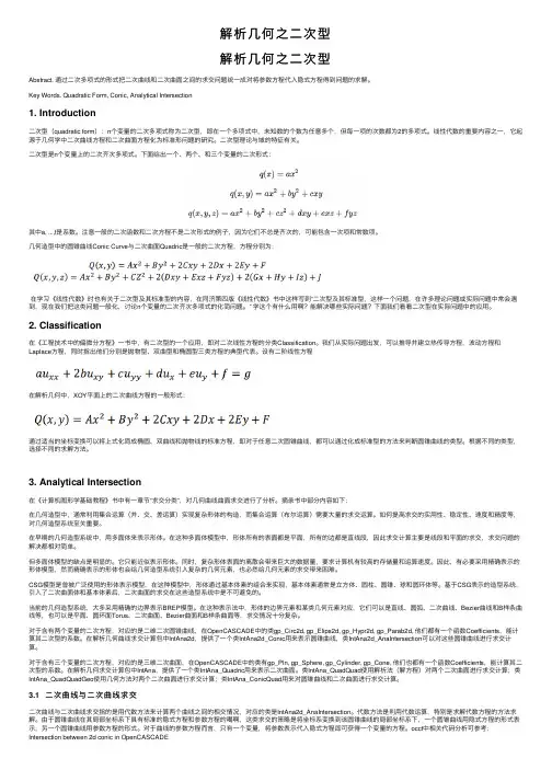
解析⼏何之⼆次型解析⼏何之⼆次型Abstract. 通过⼆次多项式的形式把⼆次曲线和⼆次曲⾯之间的求交问题统⼀成对将参数⽅程代⼊隐式⽅程得到问题的求解。
Key Words. Quadratic Form, Conic, Analytical Intersection1. Introduction⼆次型(quadratic form):n个变量的⼆次多项式称为⼆次型,即在⼀个多项式中,未知数的个数为任意多个,但每⼀项的次数都为2的多项式。
线性代数的重要内容之⼀,它起源于⼏何学中⼆次曲线⽅程和⼆次曲⾯⽅程化为标准形问题的研究。
⼆次型理论与域的特征有关。
⼆次型是n个变量上的⼆次齐次多项式。
下⾯给出⼀个、两个、和三个变量的⼆次形式:其中a, ...,f是系数。
注意⼀般的⼆次函数和⼆次⽅程不是⼆次形式的例⼦,因为它们不总是齐次的,可能包含⼀次项和常数项。
⼏何造型中的圆锥曲线Conic Curve与⼆次曲⾯Quadric是⼀般的⼆次⽅程,⽅程分别为:在学习《线性代数》时也有关于⼆次型及其标准型的内容,在同济第四版《线性代数》书中这样写到“⼆次型及其标准型,这样⼀个问题,在许多理论问题或实际问题中常会遇到,现在我们把这类问题⼀般化,讨论n个变量的⼆次齐次多项式的化简问题。
” 学这个有什么⽤啊?能解决哪些实际问题?下⾯我们看看⼆次型在实际问题中的应⽤。
2. Classification在《⼯程技术中的偏微分⽅程》⼀书中,有⼆次型的⼀个应⽤,即对⼆次线性⽅程的分类Classification。
我们从实际问题出发,可以推导并建⽴热传导⽅程,波动⽅程和Laplace⽅程,同时指出他们分别是抛物型、双曲型和椭圆型三类⽅程的典型代表。
设有⼆阶线性⽅程在解析⼏何中,XOY平⾯上的⼆次曲线⽅程的⼀般形式:通过适当的坐标变换可以将上式化简成椭圆、双曲线和抛物线的标准⽅程,即对于任意⼆次圆锥曲线,都可以通过化成标准型的⽅法来判断圆锥曲线的类型。
计算机图形学基础(第2版)课后习题答案__陆枫

第一章绪论概念:计算机图形学、图形、图像、点阵法、参数法、图形的几何要素、非几何要素、数字图像处理;计算机图形学和计算机视觉的概念及三者之间的关系;计算机图形系统的功能、计算机图形系统的总体结构。
第二章图形设备图形输入设备:有哪些。
图形显示设备:CRT的结构、原理和工作方式。
彩色CRT:结构、原理。
随机扫描和光栅扫描的图形显示器的结构和工作原理。
图形显示子系统:分辨率、像素与帧缓存、颜色查找表等基本概念,分辨率的计算第三章交互式技术什么是输入模式的问题,有哪几种输入模式。
第四章图形的表示与数据结构自学,建议至少阅读一遍第五章基本图形生成算法概念:点阵字符和矢量字符;直线和圆的扫描转换算法;多边形的扫描转换:有效边表算法;区域填充:4/8连通的边界/泛填充算法;内外测试:奇偶规则,非零环绕数规则;反走样:反走样和走样的概念,过取样和区域取样。
5.1.2 中点Bresenham 算法(P109)5.1.2 改进Bresenham 算法(P112)习题解答习题5(P144)5.3 试用中点Bresenham算法画直线段的原理推导斜率为负且大于1的直线段绘制过程(要求写清原理、误差函数、递推公式及最终画图过程)。
(P111)解:k<=-1 |△y|/|△x|>=1 y为最大位移方向故有构造判别式:推导d各种情况的方法(设理想直线与y=yi+1的交点为Q):所以有:y Q-kx Q-b=0 且y M=y Qd=f(x M-kx M-b-(y Q-kx Q-b)=k(x Q-x M)所以,当k<0,d>0时,M点在Q点右侧(Q在M左),取左点 P l(x i-1,y i+1)。
d<0时,M点在Q点左侧(Q在M右),取右点 Pr(x i,y i+1)。
d=0时,M点与Q点重合(Q在M点),约定取右点Pr(x i,y i+1) 。
所以有递推公式的推导:d2=f(x i-1.5,y i+2)当d>0时,d2=y i+2-k(x i-1.5)-b 增量为1+k=d1+1+k当d<0时,d2=y i+2-k(x i-0.5)-b 增量为1=d1+1当d=0时,5.7 利用中点Bresenham 画圆算法的原理,推导第一象限y=0到y=x圆弧段的扫描转换算法(要求写清原理、误差函数、递推公式及最终画图过程)。
02-计算机图形学基础(第二版)PPT课件

透镜组
光 孔
触钮开关
导线
笔体 光导纤维
图2.3 光笔的结构
2021/7/22
7
图形输入设备
触摸屏(touch screen) 当用手指或者小杆触摸屏幕时,触点位置
便以光学的(红外线式触摸屏)、电子的(电 阻式触摸屏和电容式触摸屏)或声音的(声音 探测式)方式记录下来。
2021/7/22
8
图形输入设备
随机扫描(random-scan)的图形显示器中电 子束的定位和偏转具有随机性,即电子束的扫 描轨迹随显示内容而变化,只在需要的地方扫 描,而不必全屏扫描。
2021/7/22
31
随机扫描的图形显示器
2
Y
2
3
1
1
3
t
1
X
2
3
图2.16 随机扫描图形显示器的工作原理
2021/7/22
32
随机扫描的图形显示器
2021/7/22
52
2.4 显示子系统
光栅扫描图形显示子系统的结构 绘制流水线 相关概念
2021/7/22
53
光栅扫描图形显示子系统的结构
CPU
系统 主存
显示 控的光栅图形显示子系统
2021/7/22
54
光栅扫描图形显示子系统的结构
CPU
系统 主存
帧缓存
2021/7/22
41
液晶显示器——原理
液晶分子的排列在微弱的外部电场、磁场或者 应力、温度变化等作用下非常容易改变。当液 晶分子的某种排列状态在电场作用下变为另一 种状态时,液晶的光学性质随之改变,这种产 生光被电场调制的现象称为液晶的电光效应。
2021/7/22
计算机图形学基础教程附录(第二版)(孙家广 胡事民编著)

(4)两个矢量的点积
V1·V2=|V1||V2|cosθ=x1x2+y1y2+z1z2
其中,θ为两相量之间的夹角。
点积满足交换律和分配律:
V1·V2=V2·V1
V1·(V2+V3)=V1·V2+V1·V3
(5)两个矢量的叉积
叉积V1×V2是一个向量,而且满足:
①|V1×V2|=|V1||V2|sinθ,即以V1和V2为邻边所构成的平行四边形的面积。
齐次坐标的优点:
①它提供了用矩阵运算把二维、三维甚至高维空间中的一个点集,从一个坐标系变换到另一个坐标系的有效方法。
②它可以表示无穷远的点。n+1维的齐次坐标中如果h=0,实际上就表示了n维空间的一个无穷远点。对于齐次坐标[a,b,h],保持a,b不变,h→0的过程就表示了在二维坐标系中的一个点,沿直线ax+by=0逐渐走向无穷远处的过程。
即:
用齐次坐标表示为:
其中h=(zprp-z)/dp。
由比例关系,两者的变换公式为:
可以简单地将两者的关系表示为:
其中:
用矩阵表示为:
B.2二维图形的几何变换
正如我们在附录A中提到的那样,用齐次坐标表示点的变换将非常方便,因此在附录B中所有的几何变换都将采用齐次坐标进行运算。
二维齐次坐标变换的矩阵的形式是:
这个矩阵每一个元素都是有特殊含义的。其中 可以对图形进行缩放、旋转、对称、错切等变换; 是对图形进行平移变换;[gh]是对图形作投影变换;[i]则是对图形整体进行缩放变换。
C.3正平行投影(三视图)
投影方向垂直于投影平面的投影称为正平行投影,通常所说的三视图均属于正平行投影。三视图的生成就是把xyz坐标系的形体投影到z=0的平面,变换到uvw坐标系。一般还需将三个视图在一个平面上画出,这时就得到下面的变换公式,其中(a,b)为uv坐标系下的值,tx、ty、tz均如图C-3所示。
计算机图形学教案

装订首页
工业学院教案
课程:计算机图形学
学期:2013/14第一学期
课时:理论52,实验12
教材:计算机图形学基础教程
计算机图形学实践教程
教师:孔令德静丽亚
工业学院教案
工业学院教案
工业学院教案
工业学院教案
工业学院教案
工业学院教案
工业学院教案
工业学院教案
工业学院教案
工业学院教案
工业学院教案
工业学院教案
工业学院教案
工业学院教案
工业学院教案
工业学院教案
工业学院教案
工业学院教案
工业学院教案
工业学院教案
工业学院教案
工业学院教案
工业学院教案
工业学院教案
工业学院教案
工业学院教案
工业学院教案
工业学院教案
工业学院教案
工业学院教案
工业学院教案
工业学院教案。
2011国家精品教材名单

内蒙古大学 大连理 工大学 中国医科大学 中国医科 大 学 辽东学院
辽 宁农 业职 业 技术 学睇
电子工业 出版社
人 民卫 生 出版社 人 民卫生出版社
92
93
柏树 令 系统解剖学 (第 2版 ) (第 2版 ) 儿科 学 薛辛东 务技 能综 合实 训 ∵ 一 前厅 饭 店服 刘颖 客 房服 务
20
21
, ″
’ “
23
社会医学 (第 2版 ) 马克思主义新 闻观教程 中国新 闻传播史 (第 二版 ) 经济 学说 史 (第 二 版 ) 财产保险 (第 四版 ) 财政学 (第 六版 ) 中国法制 史 (第 三版 ) 宪法 (第 四版 ) 民法 (第 五版 ) 简明证 据 法 学 (第 二 版 ) 国际经济法 (第 三版 )
电子 工 业 出版社 高 等教 育 出版社
35
36 37 38 39 40
41
42 43
4在
45 46 47 48 49 50
51
r υ
0 乙
53
54
55
56
57 58 59
计算机 图形学基础教程 (第 2 孙家广 、胡事 民 版) 计算机 网络 与 Internet教 程 (第 张尧学 、郭 国强、 2版 ) 王晓春 、赵艳标 智 能卡技术 (第 三 版 )— — IC卡 王 爱英 与RFID标 签 建筑构造—— 材料 、构法 、节冫 姜 涌 点 (第 三版 ) 中国古典园林史 周维权 郝吉明、马广大、 大气污染控制 工程 (第 3版 ) 王书 肖 电子商务系统建设 与管理 刘军 、刘震 宇 物流 学 汝宜红 (第 二版 ) 列车制动 饶忠、彭俊彬 (第 2版 ) 数字图像处理学 阮秋 琦 集装箱运输与多式联运 (第 二 朱晓宁 版) 计算机组织与体 系结构 (第 4版 白中英 立体化教材 ) 热能与动力 工程专业英语 (第 三 阎维平 、柳成文 版) 杨 世杰 、汪矛 、邵 植物生物学 (第 2版 ) 晓 明 、李连 芳 (第 3版 ) 植 物 营养研 究方法 申建 波 、毛达如 (第 2版 ) 园林树木 学 陈有 民 运动场草坪 (第 二版 ) 韩 烈保 学校 心理 咨询 (第 二版 ) 郑 日昌、陈永胜 尹 冬冬 、谢 孟 峡 、 有机化学 (第 二版 ) (上 下册 ) 王炳 祥 (第 饪 ) 普通动物学 版 刘凌云 、郑光美 环 境科 学概 论 (第 2版 ) 杨志 峰 、刘 静玲 冯忠 良、伍新春 、 教育心理学 (第 二版 ) 姚梅林 、王健敏 (第 2版 ) 社 会心 理 学 金盛华 基础 日语综合教程
计算机图形学课后习题答案(孙家广)
第一章:P561、列出在你过去学习工作中用过与计算机图形学有关的程序c语言:#include <graphics.h>main(){int graphdriver = VGA, graphmode=VGAHI;initgraph(&graphdriver,&graphmode,””);setbkcolor(BLUE);setcolor(WHITE);setfillstyle(1,LIGHTRED);bar3d(100,200,400,350,100,1);floodfill(450,300,WHITE);floodfill(250,450,WHITE);setcolor(LIGHTGREEN);rectangle(450,400,500,450);floodfill(470,420,LIGHTGREEN);getch();closegraph();}JA V A语言:例1、画点Import java.io.*;Class point{int ax;int ay;int bx;int by;public point(int ax, int ay, int bx, int by){float k ; //计算斜率float b;k=(by-ay)/(bx-ax);b=ay-ax*k;system.out.println(“直线的方程为:y=”+k+”x”+”+”+b);}}例2、画矩形class DrawPanel extends Jpanel{public void paint(Graphics g){super.paint(g);Graphics2D g2= (Graphics 2D);Double leftx=200;Double topy=200;Double width=300;Double height=250;Rectangle2D rect= new Rectangle2D.double(leftx,topy,width,height);G2.draw(rect);}}2、列出你所用过的窗口系统中与观感有关的元素的功能,如图标、滚动棒、菜单等使用滚动条当文档、网页或图片超出窗口大小时,会出现滚动条,可用于查看当前处于视图之外的信息。
计算机图形学基础(第二版)部分习题答案
华中科技大学计算机图形学课后习题指导一、第五章5.3 试用中点Bresenham算法画直线段的原理推导斜率为负且大于1的直线段绘制过程(要求写清原理、误差函数、递推公式及最终画图过程)。
分析:这是典型的算法推导题,推导时需要首先确定最大位移方向,然后根据最大位移方向确定候选点,并利用候选点的中点构造判别式;根据判别式确定选择候选点的条件,然后确定判别式的递推公式以及初值。
解:5.7 利用中点Bresenham画圆算法的原理推导第一象限x=y到y=0圆弧段的扫描转换算法(要求写清原理、误差函数、递推公式及最终画图过程)。
分析:这是典型的算法推导题,推导时需要首先确定最大位移方向,然后根据最大位移方向确定候选点,并利用候选点的中点构造判别式;根据判别式确定选择候选点的条件,然后确定判别式的递推公式以及初值。
圆算法应该注意的是算法是从理想圆与坐标轴交点开始的。
解:在x=y到y=0的圆弧中,(R, 0)点比在圆弧上,算法从该点开始。
最大位移方向为y,由(R, 0)点开始,y渐增,x渐减,每次y方向加1,x方向减1或减0。
(注意算法的起始点)设P点坐标(xi, yi),下一个候选点为Pr(xi, yi+1)和Pl(xi-1, yi+1),取Pl和Pr的中点M(xi-0.5, yi+1),设理想圆与y=yi+1的交点Q,构造判别式:d=F(xM, yM)=(x-0.5)2+(y+1)2-R2当d<0时,M在Q点左方,取Pr(xi,yi+1);当d>0时,M在Q点右方,取Pl(xi-1,yi+1);当d=0时,M与Q点重合,约定取Pl(xi-1, yi+1)。
5.11 如图所示多边形,若采用扫描转换算法(ET边表算法)进行填充,试写出该多边形的ET表和当扫描线Y=4时的有效边表(AET表,活性边表)。
分析:改进的有效边表算法是用软件方法实现扫描转换效率较高的算法,它利用了边表来构造有效边表。
需要注意的有以下几点:(1)构造边表时,水平边不需要构造,算法能够获取到水平边的两个端点,配对填充后水平边被填充,因此水平边的数据不参与计算。
计算机图形学基础教程孔令德课后答案
计算机图形学基础教程孔令德课后答案【篇一:大学计算机图形学课程设】息科学与工程学院课程设计任务书题目:小组成员:巴春华、焦国栋成员学号:专业班级:计算机科学与技术、2009级本2班课程:计算机图形学指导教师:燕孝飞职称:讲师完成时间: 2011年12 月----2011年 12 月枣庄学院信息科学与工程学院制2011年12 月20日课程设计任务书及成绩评定12【篇二:计算机动画】第一篇《计算机图形学》小结《计算机图形学》第一章:从计算机的辅助设计,艺术,和虚拟现实技术等方面介绍了计算机图形学的应用领域;接下了解了有关计算机图形学的概念和发展情况和图新显示器的发展和阴极射线管光栅扫描显示等的工作原理;最后介绍了图形学的最新技术。
第二章:介绍了面向对象程序设计,visual c++下的编程,主要基于mfc的编程,更重要的是绘制图形的方法。
第三章:图形的扫描与转换:主要分两部分,一是:直线,圆,和椭圆的扫描和转换中的一些重要而经典的算法。
二是:反走样技术,尤其,直线距离加权反走样的算法。
第四章:主要介绍了多边形填充,有多边形的的概述到有效边表填充,边缘填充,最后区域填充的原理和算法第五章:二维变换和裁剪:主要介绍了裁剪的方法:cohen sutherland算法是最著名的算法,除此之外还有重点分割裁剪算法,梁友栋——barsky算法。
第二篇计算机动画2.1计算机动画的概念:计算机动画是指采用图形与图像的处理技术,借助于编程或动画制作软件生成一系列的景物画面,其中当前帧是前一帧的部分修改。
计算机动画是采用连续播放静止图像的方法产生下图1-1几幅图片就是用计算机动画(a)(b)(c)(d)图2-1 计算机动画示例2.2 计算机动画的发展:计算机动画的发展大致分为三阶段:第一阶段:初出茅庐阶段:20世纪60年代初。
第一部计算机动画片诞生,之后大约20年,二维动画是计算机动画研究的重心,同时,二维动画也被应用于教学演示和辅助传统的动画片制作。
清华-计算机图形学chap7-B-Spline-2
Computer GraphicsShi-Min HuShi Min HuTsinghua UniversityTsinghua UniversityToday s TopicsToday’s Topics•Why splines?•B-Spline Curves and properties •B-Spline surfacesB Spline surfaces•NURBS curves and SurfacesWhy to introduce B Spline(BWhy to introduce B-Spline (B样条)•Bezier curve/surface has many advantages, but they have two main shortcomings:e e cu ve/su ace ca ot be od ed oca y–Bezier curve/surface cannot be modified locally(局部修改).–It is very complex to satisfy geometric continuityIt i l t ti f t i ti itconditions for Bezier curves or surfaces joining.•History of B-splinesI1946S h b d li b d–In 1946, Schoenberg proposed a spline-basedmethod to approximate curves.–It’s motivated by runge-kutta problem ininterpolation: high degree polynomial may surge p g g p y y g upper and down–Why not use lower degree piecewise polynomial Wh t l d i i l i lwith continuous joining?–that’s Spline–But people thought it’s impossible to use Spline in shape design because complicatedin shape design, because complicated computation–In 1972, based on Schoenberg’s work, Gordon I1972b d S h b’k G d and Riesenfeld introduced “B-Spline” and lots of corresponding geometric algorithms.f di i l i h–B-Spline retains all advantages of Bezier curves, and overcomes the shortcomings of Bezier curves.•Tips for understanding B-Spline?–Spline function interpolation is well known, it can Spline function interpolation is well known it canbe calculated by solving a tridiagonalequations(三对角方程).i–For a given partition of an interval, we cancompute Spline curve interpolation similarly.–All splines over a given partition will form aAll splines over a given partition will form alinear space. The basis function of this linearspace is called B-Spline basis function.i ll d B S li b i f i–Similar to Bezier Curve using Bernstein basis functions, B-Spline curves uses B-Spline basis f nctions B Spline c r es ses B Spline basis functions.B-Spline curves and it’s p Properties•Formula of B-Spline Curve.n ]1,0[),()(,0∈=Σ=t t B P t P n i i n i are control points ∑==i k i i t N P t P 0,)()(–are control points. –(i=0,1,..,n) are the i-th B-Spline basis function ),,1,0(n i P i L =)(,t N k i of order k. B-Spline basis function is a order k (degree k -1) piecewise polynomial (分段多项式) determined by the knot vector, which is a non-decreasing set of numbers.g•Demo of B-splineThe story of order & degree•The story of order°ree–G Farin: degree, Computer Aided Geometric Design –Les Piegl: order, Computer Aided DesignL Pi l d C Aid d D iB Spline Basis Function B-Spline Basis Function•Definition of B-Spline Basis Function –de Boor-Cox recursion formula:⎧⎩⎨<<=+Otherwiset x t t N i i i 01)(11,−−,,11,111()()()i i k i k i k i k i k i i k i t t t t N t N t N t t t t t +−+−+−++=+−−–Knot Vector: a sequence of non-decreasing number L L L k n k n n n k k t t t t t t t t +−++−,,,,,,,,,,11110L L L•, i = 01k=•, i = 02k=⎧⎩⎨<<=+Otherwiset x t t N i i i 01)(11,,,11,111()()()i i k i k i k i k i k i i k i t t t t N t N t N t t t t t +−+−+−++−−=+−−B Spline Basis Function B-Spline Basis Function•Questions:–What is nonzero domain(非零区间) of B-Splinebasis function ?)(,t N k i –How many knots does it need?Wh t i th d fi iti d i ()f th –What is the definition domain(定义区间) of the curves?4,4()()i i P t PN t =∑0i =B Spline Basis Function B-Spline Basis Function•take k=4, n=4 as example 4,4()()i i P t PN t =∑876543210,,,,,,,,t t t t t t t t t 0i=B Spline Basis Function B-Spline Basis Function•Properties:N ti it d l l t–Non-negativity and local support •is non-negativeis a non ero pol nomial on ,()i k N t ]•is a non-zero polynomial on ⎧∈≥+t t t t N k i i ],[0[,i i k t t +,()i k N t –Partition of Unity⎩⎨=otherwisek i 0)(,•The sum of all non-zero order k basis functions onis 1 ∑n 11[,]k n t t −+=+−∈=i n k k i t t t t N011,],[1)(B Spline Basis Function B-Spline Basis Function•Properties:Diff ti l ti f th b i f ti–Differential equation of the basis function:,,11,11111()()()i k i k i k i k i i k i k k N t N t N t t t t t −+−+−++−−′=+−−–Please compare with the Bernstein base:)]B 10 )],()([)(1,1,1,n i t B t B n t n i n i n i ⋅⋅⋅=−=′−−−;,,,B SplineB-Spline•Category(分类) of B-Splineg g p–General Curves could be categorized to two groups by checking if the start point and the endpoint areoverlapped:•Open Curves•Close CurvesClose Curves–According to the distribution(分布) of the knots inknot vector, B-Spline could be classified to theknot vector B Spline could be classified to thefollowing four groups:Uniform B-Spline(均匀B样条)U if B S li–(1) Uniform B-Spline,,,,,,,,•The knots are uniformed distributed, like 0,1,2,3,4,5,6,7•This kind of knot vector defines uniform B-Spline basisfunctionuniform B-Spline of Degree 3if B S li f D3Quasi Uniform B Spline(Quasi-Uniform B-Spline(准均匀B样条)–(2) Quasi-Uniform B-Splinep•Different from uniform B-Spline, it has:–the start-knot and end-knot have repetitiveness(重复度) of k–Uniform B-Spline does not retain the “end point” property ofBezier Curve, which means the start point and end point ofuniform B-Spline are no-longer the same as the start point andend point of the control points. However, quasi-Uniform B-end point of the control points However quasi Uniform BSpline retains this “end point” propertyQuasi-uniform B-Spline curve of degree 3Piecewise Bezier Curve(Piecewise Bezier Curve(分段Bezier曲线)–(3) Piecewise Bezier Curvep()•the start-knot and end-knot have repetitiveness(重复度)of kp•all other knots have repetitiveness of k-1•Then each curve segment will be Bezier curvesPiecewise B-Spline Curve of degree 3Piecewise Bezier Curve(分段Bezier曲线) Piecewise Bezier Curve(•For piecewise Bezier curve, the different pieces of th l ti l i d d t M i ththe curve are relatively independent. Moving the control point will only influence the corresponding piece of curve, while other pieces of curves will be not change. Furthermore, the algorithms for Bezier not change.Furthermore,the algorithms for Bezier could also be used for piecewise Bezier Curve.•But this method need more data to define the curve (more control points, more knots).Non-uniform B-Spline (非均匀B p (样条)–(4) Non-uniform B-Spline•The knot vectors satisfy T t t t =L e o vec o s sa s y conditions that the sequence of knots is non-)01[,,,]n k +decreasing(非递减). –repetitiveness of two end knots, <= k –repetitiveness of other knots, <= k-1•This kind of knot vector defines the non-uniformB-Spline.Properties of B Spline Curves Properties of B-Spline Curves•Properties of B-Spline curvesL l(–Local(局部性)•The curve in interval is only affected ],[1+∈i i t t t by at most k control points , and is independent of other control points.),,1(i k i j P j L +−=•Changing the position of control point will only affect the curve on interval i P only affect the curve on interval),(k i i t t +n∑==i k i i t N P t P 0,)()(Properties of B Spline Properties of B-Spline–Continuity(连续性)P()i i d f i i•P(t) is continuous at a node of repetitiveness r.–Convex hull(凸包性)1k r C −−•A B-spline curve is contained in the convex hullof its control polygon More specifically if t is of its control polygon. More specifically, if t is in knot span , then P(t) is in the h ll f t l i t n i k t t i i ≤≤−+1),,(1convex hull of control points ik i P P ,,1L +−Properties of B Spline Properties of B-Spline–Piecewise polynomial (分段多项式)•In every knot span, P(t) is a polynomial of t whose y p ()p ydegree is less than k.–Derivative formula(Derivative formula(导数公式)′′nn)()()(0,0,'===⎟⎠⎞⎜⎝⎛=∑∑i k i i i k i i t N P t N P t P ],[)()1(111,111+−−=−+−∈⎟⎟⎠⎞⎜⎜⎝⎛−−−=∑n k k i ni i k i i i t t t t N t t P PkProperties of B SplineProperties of B-Spline–Variation Diminishing Property(变差缩减性)•this means no straight line intersects a B-splinethi t i ht li i t t B licurve more times than it intersects the curve'scontrol polygons.t l l–Geometry invariability(几何不变性)•The shape and position of curve are independentwith the choosing of coordinate system(坐标系).Properties of B Spline Properties of B-Spline–Affine invariability(仿射不变性)nI h h f f i i i i bl d h∑=+−∈=i n k k i i t t t t N P A t P A 011,],[,)(][)]([•It means that the form of equation is invariable under the affine transformation.–Line holding(直线保持性)•It means that if the control polygon degenerates to a line,the B-Spline curve also degenerates to a line.Properties of B Spline Properties of B-Spline–Flexibility(灵活性)U i B S li C il t t•Using B-Spline Curve we can easily construct special cases such as line segment(线段), cusp(尖)t t li ()点), tangent line(切线).•For example, for B-Spline of order 4 (degree 3), if li l dyou want to construct a line segment, you only need to specify collinear (共线). 321,,,+++i i i i P P P P •you only need to let12i i i P P P ++==Properties of B Spline Properties of B-Spline相•If you want the curve tangent(相切) to a specific line L,you only need to specify on line L, and21,,++i i i P P P repetitiveness of less than 2.3+i t iP 1+i P 2+i P P )(tPP 4+i (a)四顶点共线(b)二重顶点和三重顶点−i P 23()重节点和三重节点(c)二重节点和三重节点(d)三顶点共线图.1.26 三次B样条曲线的一些特例De Boor Algorithm De Boor Algorithm•To compute P(t) (a point on the curve), you could use B-Spline formula, but it is more efficient to use de pBoor algorithm.De Boor Algorithm:•De Boor Algorithm:)()()(,,==∑∑jki ink i i t NP t N P t P 10−+−+−==⎤⎡−+−=jk i i k j i i t N tt t N t t P )()(111,111,1−++−=+++−+⎤⎡−−⎥⎦⎢⎣−−∑jk i i k j i k i i k i k i i k i i t t t t t t t t ],[)(11,1111+−+−=−−+−+∈⎥⎦⎢⎣−+−=∑j j k i k j i i i k i i i k i t t t t N P t t P t tDe Boor Algorithm De Boor Algorithm•Let⎧⋅⋅⋅+−+−==k k i r P ,,2,1,0,⎪⎪⎨−−+−−=−−−+−t P t t t t t P t t t t jj j t P r i r k i r i i i r i ),()()(]1[1]1[][•Then⎪⎪⎩⋅⋅⋅++−++−=−⋅⋅⋅=−+−+j r k j r k j i k r ir k i i r k i ,,2,1;1,,2,1∑∑−==jk i ijki it N t Pt NP t P 1,]1[,)()()()(•This is De Boor Algorithm.+−=+−=k j i k j i 21De Boor Algorithm De Boor Algorithm•The recursion of De Boor Algorithm is as shown below:01P P 1[1]j k P −+M 22[1][2]333j k j k j k j k j k P PP P P −+−+−+−+−+→→→[1][2][1]k j jjjP PPP−→→M M M M nP MDe Boor Algorithm De Boor Algorithm•Geometric meaning (几何意义)of De Boor Algorithm–It has an intuitive geometric interpretation: corner g pcutting (割角).•It means that using line segment to cut][][r r It means that using line segment to cut corner . Begin frompolygon1i i P P +]1[−r i P ⋅⋅⋅polygon , after k-1 steps of cutting, fi ll i j k j k j P P P +−+−21P −P P j we finally get point on the curve P(t).)(]1[t r j +−k j P −P]1[P 4+−k j 1+−k j 2+k j jKnot Insertion Knot Insertion •Knot insertion–An important tool for practical interactive use of B-p pspline, which allows one to add a new knot to a B-spline without changing the shape or its degree.For spline without changing the shape or its degree. For instance, one may want to insert additional knots in order to be able to raise flexibility of shape control order to be able to raise flexibility of shape control.•Insert a new knot t to a knot span Th k t t b[]1,+i i t t •The knot vector becomes:[]k n i i t t t t t t T ++=,,,,,,,1101L L •denoted as:[]11121111101,,,,,,,1++++=k n i i i tt t t t t T L LKnot Insertion Knot Insertion•The new knot sequence defines a new group of B-Spline Basis F nctions The original c r e Spline Basis Functions. The original curve P(t)can be expressed by this new group of BasisFunctions and new control points , which are unknown.1jP +=111n t N P t P ∑=0,)()(j kjjKnot Insertion Knot Insertion•Boehm gives a formula for computing new control points:p ⎪⎧+−==1,,1,0 ,11k i j P P j j L ββ⎪⎩⎨++−==−+−=+−=−−1,,1 ,,,2 ,)1(111n r i j P P r i k i j P P P j jj j j j j L L ββj t t −=β•r is the repetitiveness of newly inserted knot in the knot jk j j t t −−+1s t e epet t ve ess o ew y se ted ot t t e ot sequence.Knot Insertion Knot Insertion1P 1P P 1P 03i points(totally k-1points)36points( totally k 1 points) are replaced by the right ones(totally k points)],[43t t t ∈See demo of knot insertionB Spline Surface(B B-Spline Surface(B样条曲面)•Given knot vectors in axes(参数轴) U and V:],,,[10p m u u u U +=L B S li f f d i d fi d],,,[10q n v v v V +=L •B-Spline surface of order p ×q is defined as:m n∑∑===i j q j p i ij v N u N P v u P 00,,)()(),(B Spline Surface B-Spline Surface•are the control points of B-Splineij P Surface, which are usually referred to as thecontrol net ).(控制网格、特征网格)•and are B-Spline basis)(,u N p i )(,v N q j functions of order p and q , one for each direction (and ),which could also be direction (U and V ), which could also be computed by de Boor-Cox formula.B Spline Surface B-Spline Surface03P 23P33P02P 22P 12P32P01P 11P 21P 31P P 10P 20P 0030PNURBS Curve and SurfaceNURBS Curve and Surface •Disadvantage of B-Spline curve and Bezier Curve:–can’t accurately represent conic(圆锥曲线) curveexcept parabola(抛物线),NURBS (Non Uniform Rational B Spline) •NURBS(Non-Uniform Rational B-Spline) (非均匀有理B样条)–In order to find a mathematical method that couldrepresent conic and conicoid(二次曲面) accurately. yNURBS•NURBS is too complex•Les Piegl s The NURBS Book,Les Piegl’s The NURBS Book–“NURBS from Projective Geometry to Practical Use”–Les Piegl,Graduated from Budapest University ofi l d d f d i i fHungary, many years in SDRC company for geometricmodeler designd l d iNURBSSome years ago a few researchers joked about NURBS,saying that the acronym really stands for NOBODYUnderstands Rational B-Splines, write the authors in their foreword; they formulate the aim of changing NURBS to EURBS, that is, Everybody.…There is no doubt that they have achieved this goal....I highly recommend the book to anyone who is interestedp y p in a detailed description of NURBS. It is extremely helpful for students, teachers and designers of geometric modeling ysystems. ——Helmut PottmannNURBS•Advantages of NURBS–It provide a general and accurate representation forrepresenting and designing free curves or surfaces(自由曲线曲面)–They offer one common mathematical form for bothstandard analytical shapes (e.g., conics) and free-formshapes (parametric form).–can be evaluated reasonably fast by numerically stableand accurate algorithms;NURBS•Advantages of NURBS–They are invariant under affine as well as perspectivetransformations.–the control points and weights can be modified, whichgives great flexibility for designing curves/surfaces.–non-rational B-Spline, non-rational and rational Beziercould be viewed as special cases of NURBS.NURBS•Some difficult problems in using NURBS –Require more storage than traditionalcurve/spline methods. (such as circle representation) p–If the weights are set inappropriately, the curvewill be abnormal(畸变).will be abnormal()–It is very complex to deal with situations likecurve overlap(曲线重叠).NURBS •Before discussing about NURBS, let’s first review the definition of B-Spline:n∑==i k i i t N P t P 0,)()()()()(1,111,1,t N t t t t t N t t t t t N k i i k i k i k i i k i i k i −++++−−+−−+−−=k n k n n n k k t t t t t t t t +−++−,,,,,,,,,,11110L LLNURBS•Definition of NURBS curve.–NURBS Curves are defined by piecewiserational B-Spline polynomial basis functionp p y(分段有理B样条多项式基函数):∑== =nnikiiitNP,)(ω∑∑==ikiinikiitRPtNtP,0,)( )()(ω=nki ik itNtR, ,)()(ω∑=jkjjt N,)(ωDefinition of NURBS Definition of NURBS•NURBS basis R i,k (t) retains all properties of B-Spline Basis.–Local support: Ri,k(t)=0,t ∉[ti, ti+k]–Partition of Unity:∑n Partition of Unity:–Differentiability(可微性): If is not a knot is infinitely differentiable()==i k i u R 0,1)(•If t is not a knot, P(t)is infinitely differentiable(无限次可微) in the knot interval. If t is a knot, P(t) is only C-(k-r) continuous.continuous. –If ωi =0, then R i,k (t)=0;If +th R (t)1–If ωi =+∞, then R i,k (t)=1;Definition of NURBSDefinition of NURBS•NURBS curve has similar geometric properties as the B Spline C r e:the B-Spline Curve:–Local support (局部支持性).–Variation Diminishing Property(变差缩减性)–Strong Convex hull(凸包性)–Affine invariability(仿射不变性)–Differentiability(y(可微性)–If the weight of a control point is 0, then correspondingcontrol point doesn t affect the curve.control point doesn’t affect the curve.Definition of NURBS Definition of NURBS–If , and , then N i l/i l B i d ∞→i ω],[k i i t t t +∈i P t P =)(–Non-rational/rational Bezier curves and non-rational B-Spline curves are special cases ofNURBS curve.。