系统动力学模型构建与Vensim软件应用教程
系统动力学及vensim建模与模拟技术

系统行为分析
预测系统行为
在构建系统动力学模型时,需要对系统的行为进行预测和分析,了 解系统在不同条件下的响应和变化规律。
分析行为特征
通过对系统行为的深入分析,可以了解系统的动态特性和变化趋势, 为模型建立提供依据。
确定行为目标
在分析系统行为的基础上,需要确定系统的行为目标,即希望系统 达到的状态或结果,以便对模型进行有效的优化和控制。
定义模型规则
根据系统行为的特点,定义模型规则,如时 间延迟、逻辑规则等。
参数化模型
根据已知数据和经验,为模型中的参数赋值。
模型验证与测试
01
模型验证
通过对比历史数据和模拟结果,验 证模型的准确性和可靠性。
模型测试
通过多种情景模拟,测试模型的预 测能力和适用范围。
03
02
敏感性分析
分析模型对参数变化的敏感性,了 解参数对系统行为的影响。
详细描述
城市交通系统是一个复杂的网络,包括道路、交通信号、车辆、行人等。通过 建立城市交通系统模型,可以模拟不同交通政策或基础设施改进方案的效果, 为城市交通规划提供决策支持。
案例三:企业运营系统模拟
总结词
企业运营系统模拟是应用系统动力学和Vensim建模与模拟技术的实际应用案例 ,用于优化企业资源配置和提高运营效率。
03 系统动力学模型构建
系统边界设定
1 2
确定研究范围
在构建系统动力学模型时,首先需要明确系统的 研究范围,即确定系统的边界,以避免不必要的 复杂性和不确定性。
排除外部因素
在设定系统边界时,应将注意力集中在系统内部 的相互关系上,暂时忽略外部因素的影响。
3
确定主要变量
在确定系统边界后,应确定对系统行为有重要影 响的主要变量,这些变量将成为模型中的状态变 量。
系统动力学vensim软件使用说明
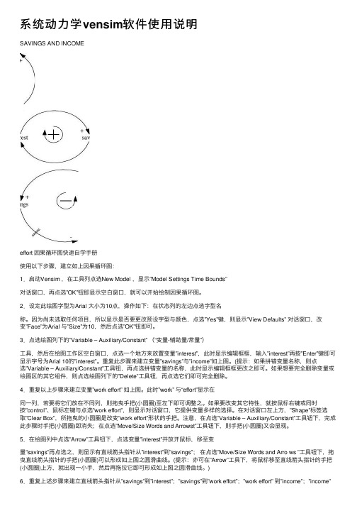
系统动⼒学vensim软件使⽤说明SAVINGS AND INCOMEeffort 因果循环图快速⾃学⼿册使⽤以下步骤,建⽴如上因果循环图:1.启动Vensim ,在⼯具列点选New Model ,显⽰”Model Settings Time Bounds”对话窗⼝,再点选”OK”钮即显⽰空⽩窗⼝,就可以开始绘制因果循环图。
2.设定此绘图字型为Arial ⼤⼩为10点,操作如下:在状态列的左边点选字型名称。
因为尚未选取任何项⽬,所以显⽰是否要更改预设字型与颜⾊,点选”Yes”键,则显⽰”View Defaults” 对话窗⼝,改变”Face”为Arial 与”Size”为10,然后点选”OK”钮即可。
3.点选绘图列下的”Variable – Auxiliary/Constant” (“变量-辅助量/常量”)⼯具,然后在绘图⼯作区空⽩窗⼝,点选⼀个地⽅来放置变量”interest”,此时显⽰编辑框框,输⼊”interest”再按”Enter”键即可显⽰字号为Arial 10的”interest”。
重复此步骤来建⽴变量”savings”与”income”如上图。
(提⽰:如果拼错变量名称,则点选”Variable – Auxiliary/Constant”⼯具钮,再点选拼错变量的名称,此时显⽰编辑框框更改之即可。
如果想要完全删除变量或绘图区的其它组件,则点选绘图列下的”Delete”⼯具钮,再点选它们即可完全删除。
4.重复以上步骤来建⽴变量”work effort” 如上图。
此时”work” 与“effort”显⽰在同⼀列,若要将它们放在不同列,则拖曳⼿把(⼩圆圈)⾄左下即可调整之。
如果要改变其它特性,就按⿏标右键或同时按”control”、⿏标左键与点选”work effort”,则显⽰对话窗⼝,它提供变量多样的选择。
在对话窗⼝左上⽅,”Shape”标签选取”Clear Box”,所拖曳的⼩圆圈是改变”work effort”形状的⼿把。
系统动力学模拟软件Vensim使用指南
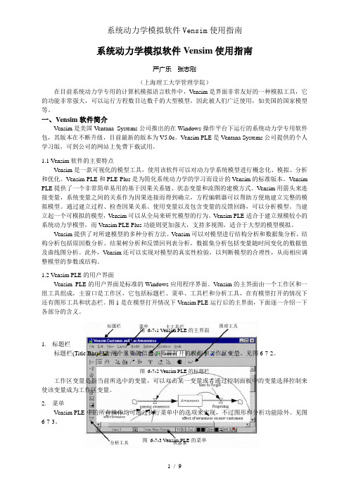
系统动力学模拟软件Vensim使用指南严广乐张志刚(上海理工大学管理学院)在目前系统动力学专用的计算机模拟语言软件中,V ensim是界面非常友好的一种模拟工具,它的功能非常强大,可以运行方程数目达数千的大型模型,因此被人们广泛使用,如美国的国家模型等。
一、Vensim软件简介Vensim是美国Ventana Systems公司推出的在Windows操作平台下运行的系统动力学专用软件包,其版本在不断升级,目前最新的版本为V5.0c。
Vensim PLE是Ventana Systems公司提供的个人学习版,可到公司的网站上免费下载试用。
1.1 Vensim软件的主要特点Vensim是一款可视化的模型工具,使用该软件可以对动力学系统模型进行概念化、模拟、分析和优化。
Vensim PLE和PLE Plus是为简化系统动力学的学习而设计的Vensim的标准版本。
Vensim PLE提供了一个非常简单易用的基于因果关系链、状态变量和流图的建模方式。
Vensim用箭头来连接变量,系统变量之间的关系作为因果连接而得到确立,方程编辑器可以帮助方便地建立完整的模拟模型。
通过建立过程、检查因果关系、使用变量以及包含变量的反馈回路,可以分析模型。
当建立起一个可模拟的模型,Vensim可以从全局来研究模型的行为。
Vensim PLE适合于建立规模较小的系统动力学模型,而Vensim PLE Plus功能则更加强大,支持多视图,适合于大型的模型模拟。
Vensim提供了对所建模型的多种分析方法。
Vensim可以对模型进行结构分析和数据集分析,结构分析包括原因数分析、结果树分析和反馈回列表分析,数据集分析包括变量随时间变化的数据值及曲线图分析。
此外,Vensim还可以实现对模型的真实性检验,以判断模型的合理性,从而相应调整模型的参数或结构。
1.2 Vensim PLE的用户界面Vensim PLE的用户界面是标准的Windows应用程序界面。
第6讲_系统动力学及Vensim建模 PPT
系统动力学的系统观点基础
系统可以用一组随时间变化的状态变量X=(x1,x2,..n)描述:系统的相空间 系统有一定的输入: U=(u1, u2, ..,um): 控制量 系统是通过相互作用而发展变化的:X’=f(X,U,t)
X`(x1`,x2`,...,xn`)
X(x1,x2,..,xn)
U(u1,u2,...,um)
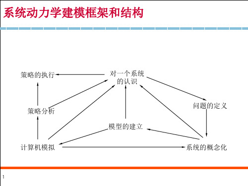
系统动力学建模框架和结构
策略的执行 策略分析
计算机模拟
对一个系统 的认识
模型的建立
问题的定义 系统的概念化
系统动力学解决问题的一般过程
提出 问题
参考行为 模式分析
提出假设 建立模型
模型 模拟
得到 结论
▪ 提出问题:明确建立模型的目的。即要明确要研究和解决什么问题。
▪ 参考行为模式分析:分析系统的事件,及实际存在的行为模式,提出设 想和期望的系统行为模式。作为改善和调整系统结构的目标。
Vensim 软件的历史
Vensim 软件的历史
(4)简单系统与行为 一阶系统系统行为 二阶系统系统及行为
(1) 系统动力学简介
系统动力学发展历史 系统动力学主要应用领域 系统动力学基本观点 系统动力学学科基础 系统动力学建模基本过程
系统动力学发展历史
MIT和福瑞斯特(Jay W. Forrester)
1950~60年代SD诞生
工业动力学、城市动力学
第6讲_系统动力学及Vensim建模
主要内容
(1)系统动力学简介 系统动力学发展历史 系统动力学主要应用领域 系统动力学学科基础 系统动力学建模基本过程
(2)Vensim 软件简介 软件配置 基本功能 用户界面 模型库及辅助知识
(3)系统动力学及Vensim建模基础 因果链与反馈 因果回路图构建 流图构建
系统动力学及Vensim建模与模拟技术PPT课件

主要内容Βιβλιοθήκη (1)系统动力学简介 系统动力学发展历史 系统动力学主要应用领域 系统动力学学科基础 系统动力学建模基本过程
(2)Vensim 软件简介 软件配置 基本功能 用户界面 模型库及辅助知识
(3)系统动力学及Vensim建模基础 因果链与反馈 因果回路图构建 流图构建
3
Page 3
15
系统动力学建模流程
任务调研 问题定义 划定界限
系统分析
反馈结构分析 变量定义
结构分析
建立方程
建立模型
模型模拟
模型评估
政策分析与模型使用
修改模型
16
Page 16
系统动力学数学描述
Page 17
根据分解原理
系统S划分成若干个(p个)相互关联的子系统(子结构)St。
式中:
SSiS1p
S——代表整个系统;
24
Page 24
Vensim 软件的历史
Vensim 专利技术
Causal Tracing™ Subscripting Optimization Venapp Flight Simulators
(Learning Environments) Resource Allocation algorithm
技术科学和基础理论。主要有反馈理论、控制理论、控制论、信息沦、非 线性系统理论,大系统理论和正在发展中的系统学。
应用技术——第三层次。为了使系统动力学的理论与方法能真正用于分析 研究实际系统,使系统动力学模型成为实际系统的“实验室”,必须借助 计算机模拟技术。
13
系统动力学建模框架和结构
策略的执行 策略分析
数学工具选择的指导思想(以模拟为主、演绎为辅) 模型的精度与控制(社会复杂系统应用中建模与成本控制)
系统动力学及Vensim建模与模拟技术
R1 实际库存 发货 满足顾客订货时间 结存订单 发货2
顾客订货速率
20
变量与方程建立
Page 21
变量
状态变量
Level或积分量 是单位时间变化量 是单位时间变化量
速率变量
辅助变量
21
应用例举(库存与劳动力模型)
Page 22
确定问题
问题的定义 参考模式 构模目的与使用模型的用户持点(关注两者的变化关系) 系统的界限 (库存、劳动力) 系统的反馈结构 (以库存和劳动力为主的因果反馈回路分析)
Vensim软件的界面
Page 9
标题栏:Titel Bar 菜单栏: Menu 工具栏 :Tools Bar
Main Tools Simulation Tools Analysis Tools Sketch Tools
状态栏 :Status Bar 流图区
9
Vensim软件的界面
订货增加
库存减少
订货 -
减少交 货延迟
库存增加
16
因果回路图分析(分析的基本技巧)
Page 17
因果链极性
因果链A→+ B:连接A与B的因果链取正号,
– (1)若增加A使B也增加,或 – (2)若A的变化使B在同一方向上发生变化。
因果链A→- B:连接A与B的因果链取负号,
– (1)若A的增加使B减少,或 – (2)若A的变化使B在相反方向上发生变化。
水位差 + 决定添水
18
流图构建(模型的实质性)
Page 19
系统动力学认为反馈系统中包含连续的,类似流体流动与积累过程。 速率或称变化率,随着时间的推移,使状态变量的值增或减。
系统动力学模型构建与Vensim软件应用教程
系统动力学模型构建与Vensim 软件应用教程第一部分系统动力学与Vensim 软件一、系统动力学概述系统动力学(SystemDynamics)是一门分析研究信息反馈系统的学科,也是一门认识系统问题和解决系统问题交叉的综合性的新学科。
系统动力学认为,系统的行为模式与特性主要地取决于其内部的动态结构与反馈机制。
系统:相互作用诸单元的复合体,例如:社会、经济、生态系统。
反馈:系统内同一单元或同一子块其输出与输入间的关系。
对整个系统而言,"反馈"则指系统输出与来自外部环境的输入的关系。
反馈可以从单元或子块或系统的输出直接联至其相应的输入,也可以经由媒介其他单元、子块、甚至其他系统实现。
所谓反馈系统就是包含有反馈环节与其作用的系统。
它要受系统本身的历史行为的影响,把历史行为的后果回授给系统本身,以影响未来的行为。
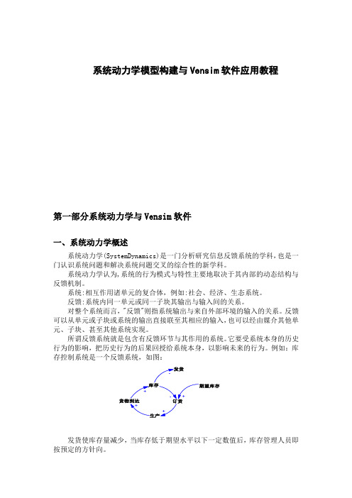
例如:库存控制系统是一个反馈系统,如图:发货使库存量减少,当库存低于期望水平以下一定数值后,库存管理人员即按预定的方针向。
生产部门订货,货物经一定延迟到达,然后使库存量逐渐回升。
反映库存当前水平的信息经过订货与生产部门的传递最终又以来自生产部门的货物的形式返回库存。
正反馈的特点是,能产生自身运动的加强过程,在此过程中运动或动作所引起的后果将回授,使原来的趋势得到加强;负反馈的特点是,能自动寻求给定的目标,未达到(或者未趋近)目标时将不断作出响应;具有正反馈特性的回路称为正反馈回路,具有负反馈特点的回路则称为负反馈回路(或称寻的回路);分别以上述两种回路起主导作用的系统则称之为正反馈系统与负反馈系统(或称寻的系统)。
回路的概念最简单的表示方法是图形,系统动力学中常用三种图形表示法:系统结构框图(structurediagram)因果关系图(causalrelationshipdiagram)流图(stockandflowdiagram)系统动力学解决问题大体可分为五步:第一步要用系统动力学的理论、原理和方法对研究对象进行系统分析。
vensim 操作手册(系统动力学)

Formulating Models of Simple SystemsusingVensim PLEversion 3.0BProfessor Nelson RepenningSystem Dynamics GroupMIT Sloan School of ManagementCambridge, MA O2142Edited by Laura Black, Farzana S. Mohamed, and students in the System Dynamics in EducationProject, April 1998.Copyright © 1998 by the Massachusetts Institute of Technology.I. Introduction and Getting StartedThe purpose of this tutorial is to help you develop some familiarity with building and analyzing system dynamics models using the Vensim PLE software. In order to become familiar with Vensim PLE, you are going to build a simple model of the federal deficit.To begin you need to get Vensim PLE ready for modeling. This tutorial makes use of the Macintosh version on Vensim PLE; the IBM-Compatible version should work similarly, but some of the screens may look different. When you first open Vensim PLE on your computer, the screen should look like this:To start working on a new model go to the File menu and select New Model. Vensim PLE will return the following dialog box:To begin your effort you must choose the time horizon of your model (when your simulation will start and finish), the appropriate time step (how accurately you wish to simulate your model), and the units of time. Start your model of the deficit in 1988 (enter 1988 in the INITIAL TIME box) and simulate it through the year 2010. Select a time step of 0.25 years. Finally, change the units of time from Month to Year. Your dialog box should now look like this:Click on OK or hit return. To give your model a name, choose the Save As... command from the File menu and enter the desired name in the text field and click on OK. (Vensim PLE should automatically supply the .mdl extension. If you are working with a different version of Vensim and see a Show all of type option on the right side of the dialog box, make sure that the .mdl Fmt Models extension is selected. This allows Vensim PLE to save the model in a format that can be used by both Macintosh and IBM-compatible computers.)∗∗ Vensim saves every simulation run and custom graph you produce as a separate file. It supplies a .vdf extension for simulation runs. These files cannot be opened from outside the Vensim application; they can be opened from inside Vensim through the Datasets / Simulate Model... and Control / Custom Graphs dialog boxes.Your screen should now look like this:You are ready to start building your model.II. Developing the Stock, Flow, and Feedback StructureThe Vensim PLE software is designed using the metaphor of a “work bench.” The large blank area in the middle of the screen is your work area, where you actually develop and analyze your model. The different buttons on the border of the work area represent the different “tools”available as you work on your model. The upper toolbar consists of the Title Bar, a Menu, a Main Toolbar, and Sketch Tools. The Main Toolbar comprises two sets of tools: file operation tools that control standard file functions—opening, closing and saving files, printing, cutting, copying, and pasting—as well as simulation and graphing tools that will allow you to set up and run simulations, and set up display graphs. The sketch tools allow you to build in model components. The tools on the Status Bar (the bottom of the window) allow you to change the formatting of the diagram. The Analysis Tools on the left on the window are tools that you will use to analyze your model to understand its behavior. You will become familiar with many of these tools as you build the deficit model.To begin, add a stock representing the outstanding federal debt to your model. Click on theYou have just created the first variable in your model, the stock of money that constitutes the federal debt.Now, add the inflow to the stock of Debt. Click on theNote: Thetool and then click on the flow valve. This action will remove the flow from the model and let you start over again.You have now created the flow, Net Federal Deficit, which increases the stock of Debt.At this point you may you wish to change the name of the stock variable from Debt to FederalDebt. Click on theNow you need to create the variables needed to determine the Net Federal Deficit. Assume the Net Federal Deficit is determined by two variables, Government Revenues and TotalGovernment Expenses. Click on thebutton to select the causal arrow tool. Now, click and release on the variable Government Revenue and then click and release again on Net Federal Deficit. Do the same for Total Government Expenses. Make sure your causal arrows actually end on the words Net Federal Deficit. They should not be attached to the cloud, the stock, or directly to the valve.You can delete arrows using theClicking on theNow, you may want to update your diagram by labeling the arrows to show that Government Revenue and Total Government Expense affect the Net Federal Deficit in different ways. Specifically, an increase in revenue causes the deficit to decrease, while an increase in expenses causes the deficit to increase. To do this, first click on thebutton on the bottom horizontal toolbar. You then see a pop-up menu that looks like this:Click and release on the desired label, and it will show up in the diagram. Label your two causal arrows so your diagram looks like this:Now, using the same steps discussed above, complete the stock, flow and feedback so your diagram looks like this:You may want to slide the handle of each arrow close to its arrowhead, so each label is clearly associated with its causal arrow.Finally, you may wish to label the positive feedback loop you have just created. Click on theClick on the Loop Clkwse button in the Shape box; click on Center in the Text Position box; and type R, for reinforcing, in the Comment box. You may also type + or P to denote a positive feedback, also known as a reinforcing, loop. Your screen should now look like this:Click on the OK button or hit return. Your screen should now appear as:III. Specifying Equations for Your ModelNow that you have developed a complete stock, flow, and feedback representation of the deficit, you need to write equations for each of the variables. Equation formulation is a critical step in the process of model building and is a key part of the process of developing a rigorous understanding of the problem at hand.To begin writing equations, click on theA highlighted variable indicates that the equation for that variable is incomplete.Variables in system dynamics models are classified as either exogenous or endogenous. Exogenous variables are those that are not part of a feedback loop, while endogenous variables are members of at least one feedback loop. Your deficit model has three exogenous variables—Government Revenue, Other Government Expenses, and the Interest Rate—and four endogenous variables—Interest Payments, Total Government Expense, Net Federal Deficit, and the Federal Debt.Start by writing the equations for the exogenous variables. To begin, click on the highlighted variable Government Revenue. You then see the following dialog box:Good modeling practice requires that each equation in a model have three elements: the equation itself, specified units of measure, and complete documentation. You enter the equation in the box to the right of the = sign. You enter the unit of measure in the text field to the right of the word Units. Equation documentation or “comment” is entered in the box to the right of the word Comment.To write an equation for Government Revenue, click in the box to the right of the = sign. Assume that government revenue is constant, so that all you need to do is enter the appropriate number for government revenue. In 1988, government revenue was about 900 billion dollars annually, so type 900000000000 in the box. Alternatively, you can write 9e11, which is Vensim PLE shorthand for 9 * 1011.Now, fill in the units. Revenue is a flow variable, so the appropriate unit of measure for this equation is dollars/time unit. Because you already chose to run the model in time steps of 1 year, the appropriate unit is dollars/year. Type dollars/year in the units field. (The next time you specify the units for a variable in this model, dollars/year will appear in the units pull-down menu. You can click on the arrowhead to the right of the units field to see units already specified for other variables in the model, and then use the mouse to select the units from that list when appropriate.) Finally, provide a description of this equation in the comment field. A good comment will be brief, but it will also give the reader the logic behind the equation as well as state the key assumptions. For example, one might write for this equation:Government revenues are assumed to be constant and equal to 900 billiondollars annually based on the actual value in 1988.Your dialog box should now look like this:Click on OK or hit return and your diagram will look like this:Government Revenue is no longer highlighted because you have just specified its equation.Following the process above, write equations for the two other exogenous variables, Interest Rate and Other Government Expenses. Use the following information:•Government expenses, excluding interest on the debt, were approximately 900 billion dollars in 1988.•The interest rate paid on the national debt in 1988 was around 7%/year.Now that the equations for the exogenous variables are formulated, turn your attention to the endogenous variables. Writing equations for the stocks and the flows is a little different, so let’s do an example of each. First we formulate the equation for the stock, Federal Debt.Again, click on theThe following dialog box will be displayed:Unlike flows and constants, a stock requires that an additional element be specified in its formulation; after you specify the equation, you need to select an initial or starting value.You enter the equation for the stock in the box to the right of the word Integ. Integ stands for “integrate” and simply means that the stock at any moment in time is equal to the sum of all the inflows minus the sum of all the outflows plus the initial value.When you created the stock, flow, and feedback diagram, you connected the flow Net Federal Deficit to the stock Federal Debt. Vensim PLE captures this stock-flow dependency by providing a list of the required Variables to the stock Federal Debt on the right side of the equation dialog box. (The variable we are formulating, Federal Debt, itself also appears in the Variables box, but we focus on the input Net Federal Deficit. In general, you will never want to have the same variable on both the left and right sides of an equation.)Because the model diagram shows the flow Net Federal Deficit feeding into the stock Federal Debt, Vensim has anticipated that the flow is an input to the stock equation and has placed the Net Federal Deficit variable name in the box to the right of Integ. If this is not the case in your version of Vensim PLE, then simply click in the box to the right of the Integ and then click on the variable Net Federal Deficit in the Variables box to write the equation for the change in Federal Debt. (Note:If Net Federal Deficit is not in the Variables box, then your model diagram is incorrect and needs to be changed—make sure the flow is attached to the stock).The Integ box should now look like this:Below the Integ box is the Initial Value box. Here you enter the initial condition or starting point for the stock. In 1988, the outstanding federal debt was approximately 2.5 trillion dollars, so enter 2500000000000 in the initial value box (alternatively you can write 2.5e12, which is Vensim PLE shorthand for 2.5 x 10¹²). The Initial Value box should look like this:Now the equation specification for the Federal Debt stock is complete. Your equation indicates that the federal debt is simply the accumulation of the Net Federal Deficit since 1988 added to the initial value.You still need to specify the unit of measure and document your equation in the comment field. The units should be fairly straightforward. The Federal Debt is a stock and its units are dollars. Useful comments briefly explain the structure of the equation and highlight the key assumptions made. A sample comment for Federal Debt is:The Federal Debt is the accumulation of the Net Federal Deficit plus theinitial value of the debt. The initial value is set to 2.5 trillion dollars,which was the approximate outstanding federal debt in 1988—the startingpoint for this simulation.Your dialog box should now look like this:Click on OK or press return.Now you need to specify the equations for the auxiliary variables and the flow.Using theThis box is identical to those used to specify the exogenous variables, but, in this case, there are two other variables in the Variables box; you are required to use these variables in the equation. When you developed the stock, flow, and feedback diagram, you drew causal arrows connecting the variable Federal Debt and constant Interest Rate to the variable Interest Payments. Vensim PLE has conveniently recognized this fact and has provided a list of the required inputs to your equation based on the picture you have already created. In fact, if you try to write your equation without using the two required variables, Vensim PLE will give you an error message. The rate of interest payment is simply equal to the current debt stock multiplied by the interest rate. To enter this equation, first click on the Federal Debt variable in the Variables box. It now appears in the equation box. Now type * (alternatively you can click on theTo complete the equation, you need to specify the units, dollars/year, and document your equation in the comment field. An appropriate comment might look like the following:The annual flow of interest payments is equal to the current outstandingfederal debt multiplied by the annual interest rate.The dialog box for the variable Interest Payments should now look like this:Following a similar process to the one outlined above, you should now be able to complete your model.IV. Using the Model Structure Analysis ToolsVensim PLE provides five tools for analyzing and understanding the structure of your model.By far the most important of these is the unit-checking tool.An important feature of any system dynamics equation is dimensional consistency, which is just a fancy way of saying that the units of measure must be the same on both the left and right sides of the equation. As an example, suppose you had chosen the units of the Federal Debt stock to be dollars and the units of the Interest Rate to be dollars/year. If so, then pressing the apple key and u (alternatively, you could select the Model menu, then select Units Check) simultaneously would yield the following message:Followed by:The problem is that, in this example, the equation for Interest Payments is not dimensionally consistent: the right and left sides of the equation have different units. The flow Interest Payments is measured in dollars per year. The Federal Debt, because it is a stock, is measuredin dollars. Multiplying Federal Debt by something with units in dollars/year results in a quantity that has units in dollars2/year—hence the error.The cause of the problem is that the unit of measure for Interest Rate is incorrect. The interest rate is not measured in dollars per year. An easy way to think about this fact is to recognize that the interest rate really has nothing to do with dollars. It could easily apply to any other currency or any other type of measurement unit. In fact, the interest rate has no unit of measure; it is dimensionless. Although it has no unit of measure, it is, nevertheless, time-dependent; an annual interest rate is not equivalent to a monthly one. As a result, the appropriate unit of measure for Interest Rate is 1/year. If you enter 1/year into the unit field of the interest rate variable and simultaneously press the apple key and u, you should receive the following message:The units in your model now balance.In this example, the unit-checking tool identified an incorrect assumption in a common mental model of the interest rate. Dimensional consistency is an important feature of system dynamics models, and Vensim PLE’s unit-checking feature often helps you to identify serious flaws in both your understanding of the system under consideration and your resulting model formulations. Always make sure that the units in your model balance!The other analysis tools that Vensim PLE provides can also be useful. Thebuttons create “causes” and “uses” trees for a variable. To use these tools, you need to first “select” a variable. To select a variable, first click on theFederal Debt, clicking on the two “causes” and “uses” buttons in sequence gives you:andThetool on the analysis tool bar identifies all the feedback loops of which the selected variable is a member.V. Simulating Your ModelVensim PLE also has tools to help you analyze the behavior of your model. Before analyzing the behavior, however, you must actually simulate the model so that you have some behavior to analyze.To run a simulation, you first need to click on the running manClicking on yes will overwrite the “current” dataset displayed in the box to the right of the running man icon. Selecting “No” will allow you to create a different dataset. It is helpful to choose names that suggest some idea of what is being tested rather than simply using name like SIM1, SIM2, etc. Because this run is the base case run for your model, you might choose to call the run BASE.* Click on No, type in BASE as your new dataset name, click on Save or hit return, and your model will start simulating.Once the simulation run is completed, you can look at the results of your simulation. Vensim PLE provides many tools with which to view simulation output. The most basic, and often the most useful, of these tools is the strip graph. To create a graph of the Federal Debt, first click on thebutton on the analysis tool bar.* Advanced Tip: Vensim PLE also offers you the choice of two numerical integration methods, Euler and Runge-Kutta 4.Runge-Kutta 4 is a more accurate integration method, but it is also more computationally intensive. Generally it is better to use the Euler method and only change if you believe you are seeing integration error.You then see:By the year 2010, given the current assumptions in the model, the federal debt will grow to more than 10 trillion dollars, four times its value in 1988.Besides the strip graph, Vensim PLE provides many other ways to examine simulation output. TheVensim PLE also can present the output in the form of a table rather than a graph. To see a table of the selected variable simply click on thebutton selected, click on Interest Rate. A dialog box will appear. In the constant box change the interest rate from 7% to 3.5%. Again, run this new simulation but do not overwrite the simulation named Base. Instead, name it interest rate.Your new graph should look like this:If you do not wish to see the previous run (base) displayed with the new simulation run, click on theA dialog box appears and shows on the left side the two simulation runs you have created so far. Double-click on the name of the simulation run you wish to remove from the graph (or highlight it and click on the << button to remove it from the right side of the dialog box). Close the Datasets window and close and re-display the strip graph. Now, only the new simulation run should appear.You may also wish to run the model for a longer period of time. In this case, selec t Time Bounds... from the Model menu. You then see the same dialog box that you saw when you first started to develop your model.You can extend your simulation by setting a new date for your final time. Run your model out to the year 2075.。
- 1、下载文档前请自行甄别文档内容的完整性,平台不提供额外的编辑、内容补充、找答案等附加服务。
- 2、"仅部分预览"的文档,不可在线预览部分如存在完整性等问题,可反馈申请退款(可完整预览的文档不适用该条件!)。
- 3、如文档侵犯您的权益,请联系客服反馈,我们会尽快为您处理(人工客服工作时间:9:00-18:30)。
系统动力学模型构建与Vensim软件应用教程
教师简介
王普,博士,讲师,北京理工大学管理科学与工程专业博士,高校教师。
课程介绍
《系统动力学模型构建与Vensim软件应用课程》主要介绍了系统动力学模型的构建过程以及借助Vensim软件实现模型的求解过程。
通过本课程的学习,一方面可以掌握系统动力学模型的基本原理和建模实现。
另一方面,可以掌握Vensim软件对系统动力学模型进行求解的操作步骤和方法。
本课程适合初学者听,听完后,可以掌握基本的系统动力学模型构建与Vensim软件操作方法与结果解读。
本教程为高清视频,画面清晰生动,身临其境。
同步教程,举一反三,效果翻倍。
可登陆中国科学软件网或科学软件学习网免费试看。
课程大纲
本视频课程分为8讲,共11个视频,时长为522分。