英文版greene 计量经济学Ch9
英文版greene 计量经济学Ch7
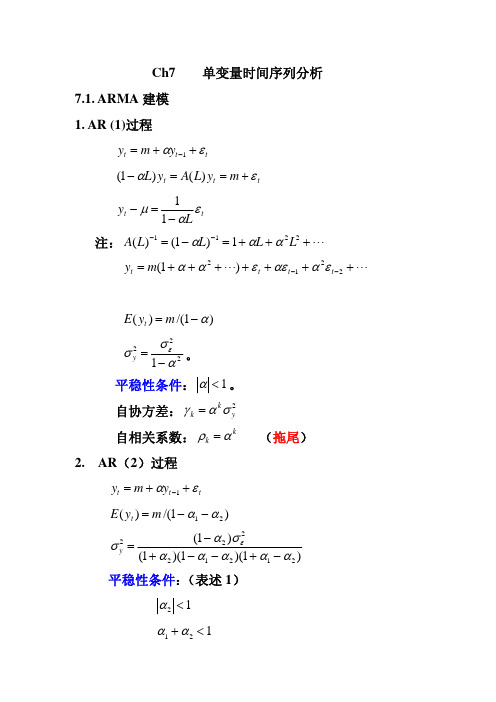
Ch7 单变量时间序列分析7.1. ARMA 建模 1. AR (1)过程t t t y m y εα++=−1t t t m y L A y L εα+==−)()1( t t Ly εαμ−=−11注: "+++=−=−−22111)1()(L L L L A ααα""+++++++=−−2212)1(t t t t m y εααεεαα)1/()(α−=m y E t2221ασσε−=y。
平稳性条件:1<α。
自协方差: 2y k kσαγ= 自相关系数: (拖尾)kk αρ=2. AR (2)过程t t t y m y εα++=−1 )1/()(21αα−−=m y E t)1)(1)(1()1(21212222ααααασασε−+−−+−=y 平稳性条件:(表述1) 12<α 121<+αα112<−αα Yule -Walker 方程: 自协方差: 12011γαγαγ+= 02112γαγαγ+= 自相关系数: 1211ρααρ+= 2112αραρ+=2111ααρ−=, 222121αααρ+−=22113−−>+=k k k ραραρ (拖尾) 滞后算子多项式的根:t t t m y L A y L L εαα+==−−)()1(221 )1)(1()(21L L L A λλ−−=24,221121αααλλ++=Ld L c L L L A 2121111)]1)(1/[(1)(λλλλ−+−=−−=−t t t t t Ld Lc x x y ελελμ212111−+−=+=−两个具有相同扰动的AR(1)过程的叠加。
特征方程:)(1221z A z z =−−αα 根:i i z λ/1= 平稳性条件:(表述2)11>z ,12>z如果出现复根,其模要小于1.即:特征方程的根位于单位园外。
计量经济学(英文版)精品PPT课件
(4.3a)
Expand and multiply top and bottom by n:
b2
=
nSxiyi - Sxi Syi nSxi2-(Sxi) 2
(4.3b)
Variance of b2
4.12
Given that both yi and ei have variance s2,
the variance of the estimator b2 is:
4. cov(ei,ej) = cov(yi,yj) = 0 5. xt c for every observation
6. et~N(0,s 2) <=> yt~N(b1+ b2xt,
The population parameters b1 and b2 4.4 are unknown population constants.
b2
+
nSxiEei - Sxi SEei nSxi2-(Sxi) 2
Since Eei = 0, then Eb2 = b2 .
An Unbiased Estimator
4.8
The result Eb2 = b2 means that the distribution of b2 is centered at b2.
4.6
The Expected Values of b1 and b2
The least squares formulas (estimators) in the simple regression case:
b2 =
nSxiyi - Sxi Syi nSxi22 -(Sxi) 2
b1 = y - b2x
《计量经济学导论》ch9

Multiple Regression Analysis: Specification and Data Issues
Example: Housing price equation
Evidence for misspecification
Discussion
Less evidence for misspecification
If the error and the proxy were correlated, the proxy would actually have to be included in the population regression function
The proxy variable is a „good“ proxy for the omitted variable, i.e. using other variables in addition will not help to predict the omitted variable
© 2012 Cengage Learning. All Rights Reserved. May not be scanned, copied or duplicated, or posted to a publicly accessible website, in whole or in part.
Multiple Regression Analysis: Specification and Data Issues
Assumptions necessary for the proxy variable method to work The proxy is „just a proxy“ for the omitted variable, it does not belong into the population regression, i.e. it is uncorrelated with its error
古扎拉蒂计量经济学第四版讲义Ch9 Model Specification

第九章模型设定Model Specification and Diagnostic Testing1. Introduction假如模型没有被正确设定,我们会遇到model specification error或model specification bias 问题。
本章主要回答这些问题:1、选择模型的标准是什么?2、什么样的模型设定误差会经常遇到?3、模型设定误差的后果是什么?4、有那些诊断工具来发现模型设定误差?5、如果诊断有设定误差,如何校正,有何益处?6、怎样评估相互竞争模型的表现(model evaluation)?Model Selection Criteria这是笼统的模型选择标准:1、利用该模型进行预测在逻辑上是可能的;2、模型的参数具有稳定性,否则,预测就很困难。
弗里德曼说:模型有效性的唯一检验标准就是比较模型的预测是否与经验一致。
3、模型要与经济理论一致。
4、解释变量必须与误差项不相关。
5、模型的残差必须是白噪声;否则就存在模型设定误差。
6、最后选择的模型应该涵盖其它可能的竞争模型;也就是说,其他模型不应该比所选模型的表现更好。
Types of specification errors大概有这几种设定误差:设定误差之一:所选模型忽略了重要的解释变量(该解释变量被包含在模型误差中)设定误差之二:所选模型包含了不必要或不相关的解释变量设定误差之三:所选模型具有错误的方程形式(比如y采用了不该采用的对数转换)设定误差之四:被解释变量and/or解释变量测量偏差(所用数据相对于真实值有偏差)导致的误差(commit the errors of measurement bias)设定误差之五:随机误差项进入模型的形式不对引起的误差(比如是multiplicatively还是additively)The assumption of the CLRM that the econometric model is correctly specified has two meanings. One, there are no equation specification errors, and two, there are no model specification errors.上面概括的五种设定误差称为equation specification errors。
Econometrics-I-9 计量经济分析(第六版英文)ppt

For the linear regression model, the distribution of the statistic is F with J and n-K degrees of freedom.
If the hypothesis is true, then the statistic will have a certain distribution. This tells you how likely certain values are, and in particular, if the hypothesis is true, then 'large values' will be unlikely.
Application: Cost Function
Price Homogeneity
Imposing the Restrictions
Homotheticity
Testing Fundamentals - I
SIZE of a test = Probability it will incorrectly reject a “true” null hypothesis.
This is the probability of a Type I error.
DENSITY
Density of F[3,100] .8
.6
.5
.3
Under the null hypothesis, F(3,100) has an degrees of freedom. Even if the null is true, F will be larger than the 5% critical value of 2.7 about 5% of the time.
计量经济学课件英文版 伍德里奇
20
1.3 The Structure of Economic Data
Cross Sectional Time Series Panel
Department of Statistics by Zhaoliqin
21
Types of Data – Cross Sectional
Department of Statistics by Zhaoliqin 10
Why study Econometrics?
An empirical analysis uses data to test a theory or to estimate a relationship
A formal economic model can be tested
Theory may be ambiguous as to the effect of some policy change – can use econometrics to evaluate the program
Department of Statistics by Zhaoliqin 11
1.2 steps in empirical economic analysis
Welcome to Econometrics
Department of Statistic:赵丽琴 liqinzhao_618@
Department of Statistics by Zhaoliqin
1
About this Course
Textbook: Jeffrey M. Wooldridge, Introductory Econometrics—A Modern Approach. Main Software: Eviews. Sample data can be acquired from internet. If time permitted, R commands will be introduced.
ch9 feenstra international economics 2 edition
Copyright © 2011 Worth Publishers·International Economics· Feenstra/Taylor, 2/e
3 of 95
FIGURE 20-1
Chapter 20: Exchange Rate Crises: How Pegs Work and How They Break
Currency Crashes In recent years, developed and developing countries have experienced exchange rate crises. Panel (a) shows depreciations of six European currencies after crises in 1992. Panel (b) shows depreciations of seven emerging market currencies after crises between 1994 and 2002.
4
5 Prepared by: Fernando Quijano
Dickinson State University
Copyright © 2011 Worth Publishers·International Economics· Feenstra/Taylor, 2/e
1 of 95
Hale Waihona Puke IntroductionCopyright © 2011 Worth Publishers·International Economics· Feenstra/Taylor, 2/e
5 of 95
Causes: Other Economic Crises
英文版greene 计量经济学Ch6
ˆ = ∑u ˆt u ˆt −1 / ∑ u ˆt2−1 ≈ 1 − ϕ
t =2 t =2
d 2
ˆ )) > 1 时,检验失效。 (1 − n var(β 1
渐进等价的检验程序:
ˆt 对 u ˆt −1 和所有回归元回归, ˆt −1 系数的显 u 检验 u
著性。 扩展到 AR(p)自回归型式:
nRe2 ~ a χ 2 (q )
(2) BPG 检验
BPG 异方差检验的思想: 对于一般多元模型 Y=Xβ+u 假定异方差由部分解释变量或全部解释变量所引起, 记其为 Z σi2=Ζα H0: α2=α3=....=αp=0
接受 H0 隐含同方差,拒绝 H0 即为异方差的证据。 定义:
ˆ /σ ˆ , pi = u
ˆ ) = ( X ' X ) −1 X 'VX ( X ' X ) −1 var(β
方差估计与标准误:
ˆ ) = ( X ' X ) −1 X 'V ˆX ( X ' X ) −1 var(β
2 2 ˆ = diag (u ˆ12 , u ˆ2 ˆn V ,", u )
∧
其标准误称为异方差一致标准误。此时,t 检 验、F 检验渐进有效。 线性约束应使用 Wald 检验:
σ t2 = α 0 + α1ut2−1 + " + α p ut2− p + γ 1σ t2−1 + " + γ qσ t2− q
估计:ML 估计。
对 AR(1)型式的自相关: ut = ϕut −1 + ε t
⎡ 1 ϕ ⎢ ϕ 1 2 var(u ) = E (u ' u ) = σ u ⎢ ⎢ # # ⎢ n −1 ϕ n−2 ⎢ ⎣ϕ
格林高级计量经济学第二版
fY ( y ) = f X ( x ) dx . dy
Remark: LHS x=x(y) “Proof”: ! By the definition of probability, within an interval ∆x : Probability = f X ( x ) ∆x Probability = fY ( y ) ∆y ⇒ f X ( x ) ∆ x = fY ( y ) ∆ y ∆x fY ( y ) = f X ( x ) ∆y ∆y dx fY ( y ) = f X ( x ) (taking limit) dy dx as a proportional factor! dy
PDF : A Function of A Random Variable Motivating example: Image that two grading systems - Chianese and American Prob { X ∈ [ 0,100]} = 1 and Prob {Y ∈ [0, 4]} = 1 How to change the PDF from Chinese to American system? Then the transformation is y=x/25 . Special case of scalar: suppose that X : f X ( x ) is known and Y is a function of X, then
a1n x1 a2n x2 ann xn ( y1 , y2 ,..., yn ) .
n
1 1 − 2 y '( AA ')−1 y fY ( y1 , y2 ,..., yn ) = e || A−1 || (一般正态分布) 2π
英文版greene 计量经济学Ch1
z= X −μ = σ/ n
n
(
X σ
−
μ)
⎯n⎯→⎯∞→
N
(0,1)
。
2.2 正态分布的线性组合
(1) 设 Zi ,i = 1,2,..n 为 n 个相互独立正态变量,其均值和
方差分别为
μ
i
,
σ
2 i
,则它们的线性组合,
∑ ∑ ∑ Z = ki Zi ~ N ( ki μi , (kiσ i )2 )
∑ σ
2 Y
=
E[(Y
− μY )2 ] =
p. j (Yj − μY )2
j
总体协方差:
∑ σ XY = E[( X − μ X )(Y − μY ))] = pij ( X i − μ X )(Yj − μY ) i
总体相关系数:
ρ XY
= σ XY σ XσY
条件概率:
P(Y j
Xi) =
pij pi.
条件期望:
∑ E(Y Xi ) = j
pij pi.
Yj
∑ 条件方差:
Var(Y Xi ) =
j
pij pi.
(Yj
−
E(Y
X i ))2
1.2 双变量正态分布
对服从联合正态分布的变量 X,Y:
联合密度函数:
f
(X ,Y)
=
1 2πσ XσY
⎧ exp⎨−
⎩
1 2(1 − ρXY 2 )
⎡ ⎢( ⎣
们的平方的和为卡方变量,即
∑Z
2 i
~
χ 2 (n)
期望:n ;方差:2n
χ 2 (n) 的概率密度函数
性质:设 Zi (i = 1,2,..n) 为相互独立且自由度分别为 ki 的卡方分
- 1、下载文档前请自行甄别文档内容的完整性,平台不提供额外的编辑、内容补充、找答案等附加服务。
- 2、"仅部分预览"的文档,不可在线预览部分如存在完整性等问题,可反馈申请退款(可完整预览的文档不适用该条件!)。
- 3、如文档侵犯您的权益,请联系客服反馈,我们会尽快为您处理(人工客服工作时间:9:00-18:30)。
Δyt = m − Πyt−1 + B1Δyt−2 + + Bp−1 yt− p+1 + ε t Π = I − A1 − Ap
特征方程: I − A1w − Ap w p = 0
讨论: (1) r(Π ) = k : yt ~ I (0) (2) r(Π ) = r < k : yt ~ I (n) ,r 个协积向量。 (3) r(Π ) = 0 : Π = 0 ,没有协积关系。
+
⎡a11 ⎢⎣a21
0 a22
⎤ ⎥ ⎦
⎡ ⎢ ⎣
y1,t −1 y2,t −1
⎤ ⎥ ⎦
+
⎡ε 1t ⎢⎣ε 2t
⎤ ⎥ ⎦
检验滞后变量系数的(联合)显著性。
3. 预测:以 VAR(1)为例
yt = Ayt−1 + ε t yn+s = As yn + As−1ε n + + ε n+s yˆn+s = As yn es = As−1ε n + + ε n+s var(es ) = As−1Ω ( A')s−1 + + Ω
回归的标准差。
等价表述: ut = Pεt
⎡ 1/ s1
P
=
⎢ ⎢
−
b21
⎣ s2.1
0⎤ ⎥
1/ s2 ⎥ ⎦
∑ P−1(P−1)'= Ωˆ = 1 n
ε
t
ε
' t
Choleski 分解。
则:εt = P−1ut ,代入 VAR 模型,计算以后各期的 y 响应。
分解次序对分解结果有显著影响。
5. 方差分解
9.2 VAR 估计
平稳时:估计 VAR
非平稳时:估计 VECM
1. 阶数判定
信息准则
似然比检验: LR = n[ln Ωˆ 0 − ln Ωˆ1 ] ~ χ 2 (q)
q = k 2 ( p0 − p1)
2. Granger 因果关系检验
⎡ ⎢ ⎣
y1t y2t
⎤ ⎥ ⎦
=
⎡m1 ⎢⎣m2
⎤ ⎥ ⎦
βˆ1 βˆ2
⎤ ⎥ ⎥
⎢⎥
=
(X 'Σ
−1 X )−1 X 'Σ
−1 y
⎢⎢⎣βˆm
⎥ ⎥⎦
var(bˆGLS ) = ( X 'Σ −1 X )−1
9.3 基于向量误差纠正模型的协整分析 确定协整秩 迹检验:备选假设:协整秩 k。 最大特征值检验:备选假设:协整秩 r+1。 估计协整向量和调节向量:ML 估计 估计误差纠正模型 例子:Example1
9.4 联立方程模型
VAR 模型的问题:自由度,多协积向量的解释
结构参数的设定和识别等。
1. 联立方程模型:
3. 估计
(1) 单方程估计——2SLS
非平稳性和协积关系不影响估计和检验的渐
进有效性——Hsiao。
(2) 系统估计——3SLS
基于 2SLS 的残差计算各方程扰动项的协方
差矩阵,进行 SUR 估计。
SUR 估计:
对方程组:
⎡ y1 ⎤ ⎡ X1 0 …
⎢ ⎢
y2
⎥ ⎥
=
⎢ ⎢
0
X2 …
⎢ ⎥⎢
0 ⎤⎡ β1 ⎤ ⎡ u1 ⎤
yt = m + Ayt−1 + ε t
令 A 的特征值与特征向量分别为:
⎡λ1 = 1
⎤
Λ
=
⎢ ⎢
λ2
⎥ ⎥
⎢⎣
λ3 ⎥⎦
C = [c1 c2 c3 ]
其中: λ2 < 1, λ3 < 1
令: zt = C −1 yt 则 z1t ~ I (1) , z2t ~ I (0) , z3t ~ I (0) 。
Ch9 多方程模型
9.1 向量自回归
yt = m + A1 yt−1 + A2 yt−2 + + Ap yt− p + ε t
E(ε t ) = 0
E
(ε
Ω ⎩⎨0,
,
t=s t≠s
1. 两变量 VAR(1)模型
⎡ ⎢ ⎣
y1 t y2t
⎤ ⎥ ⎦
=
⎡m1 ⎢⎣m2
⎤ ⎥ ⎦
+
⎡a11 ⎢⎣a21
0
⎥ ⎥
⎢ ⎢
β
2
⎥ ⎥
+
⎢ ⎢
u
2
⎥ ⎥
⎥⎢ ⎥ ⎢ ⎥
⎢⎥ ⎣ym ⎦
⎢ ⎣
0
0
…
X
m
⎥ ⎦
⎢⎣β
m
⎥ ⎦
⎢⎣um
⎥ ⎦
⎡σ 11 I
Σ
=
E (uu ' )
=
⎢⎢σ 21I ⎢
⎢⎣σ m1I
σ12 I σ 22 I
σ m2I
σ1m I ⎤
σ
2m
I
⎥ ⎥ ⎥
=
Σ
c
⊗
I
σ
mm
I
⎥ ⎦
bˆGLS
=
⎡ ⎢ ⎢
结构方程:
Byt + Cxt = ut
ut ~ iidN (0, Σ )
简约方程: yt = Πxt + vt
Π = −B−1C
vt = B −1ut
vt ~ iidN (0, Ω ) , Ω = B−1Σ (B−1)'
似然函数:
∑ L
=
p( yt
xt )
=
(2π )−n
Ω
−n / 2
exp⎢⎣⎡−
向前一期预测的方差:
Ω
=
P−1 (P −1 )' =
⎡c11 ⎢⎣c21
0 ⎤⎡v1
c2
2
⎥ ⎦
⎢ ⎣
⎤ ⎡c11
v2
⎥⎢ ⎦⎣
0
c21 ⎤
c22
⎥ ⎦
方差来源的分解:
var(yˆ11) = c121v1
var( yˆ21 ) = c221v1 + c222v2
多部预测方差的分解:
var(es ) = As−1P −1 ( As−1P −1 )' + + P −1 (P −1 )'
yt = Pzt = p1z1t + p2 z2t + p3 z3t
z2t = p(2) yt ~ I (1) , z3t = P(3) yt ~ I (0) 。 一般而言,y~I(2):
两个协积向量,一个平稳的协整关系。
3. 高阶系统
yt = m + A1 yt−1 + A2 yt−2 + + Ap yt− p + ε t
y1t 和 y2t 之间存在一个协积关系 z2t 。
误差纠正模型:
Δyt = m − Πyt−1 + ε t , Π = I − A
Π
=
I
−
A
=
C
⎡1− λ1 ⎢⎣ 0
0 1− λ2
⎤ ⎥⎦C
−1
=
[
]
[
] = αβ '
其中: β 协整向量
α 调节向量。
情形 3: λ1 = λ2 = 1 如果 A 不对称, C −1 不存在,但存在矩阵 P:
1 2
( yt − Πxt )'Ωˆ −1( yt − Πxt )⎥⎦⎤
2. 识别条件:
必要条件:阶条件——方程排斥掉的前定变量个数大于
等于方程包含的内生变量个数减 1.
充要条件:秩条件——在包含 G 个方程的系统中,方程
不含而其它所有方程所含的变量的系数矩阵中,可以构造至
少一个行列式不为 0 的 (G −1) 阶方阵。
A = PJP−1
J
=
P −1 AP
=
⎡1 ⎢⎣0
1⎤ 1⎥⎦
令: zt = P−1 yt
则: zt = m * +Jzt−1 +ηt
即:
z1t = m1 * + z1,t−1 + z2,t−1 +η1t
z2t = m2 * + z2,t−1 +η2t
则: z1t ~ I (2) , z2t ~ I (1) , yt ~ I (2) z2t ~ I (1) 是 yt ~ I (2) 的一个协积关系。 2. 三变量 VAR(1)模型
μ2 ⎥⎦
] μ3c3
⎡c ( 2) ⎢⎣c (3)
⎤ ⎥ ⎦
=
αβ
'
讨论:
λ1 = λ2 = 1, λ3 < 1
⎡1 1 0 ⎤
有非奇异矩阵 P, P−1AP = J = ⎢⎢0 1
0
⎥ ⎥
⎢⎣0 0 λ3 ⎥⎦
令: zt = P−1 yt 则 z1t ~ I (2) , z2t ~ I (1) , z3t ~ I (0)
即:
z1t = m1 * +λ1z1,t−1 +η1t
z2t = m2 * +λ2 z2,t−1 +η2t
情形 1: λ1 < 1且 λ2 < 1
zt ~ I (0) , yt ~ I (0) 。
情形 2: λ1 = 1, λ2 < 1
z1t ~ I (1) , z2t ~ I (0) , yt ~ I (1) 。
yt = Czt = c1z1t + c2 z2t + c3 z3t