最新数学建模大作业答案
《数学建模 建立函数模型解决实际问题》试卷及答案_高中数学必修第一册_人教A版
《数学建模建立函数模型解决实际问题》试卷(答案在后面)一、单选题(本大题有8小题,每小题5分,共40分)1、某公司每小时生产零件的数量与时间的关系可以用下面哪个函数模型来表示?每天工作8小时,且生产数量随着工龄增加而增加。
A、f(t) = 100 + 2tB、f(t) = 100 + 2t^2C、f(t) = 100 + 2t^3D、f(t) = 100 + 2e^t2、一个城市为了改善交通状况,计划拓宽一条现有道路。
现有道路的宽度为10米,经过调查发现,道路的宽度每增加1米,道路的日均车流量会减少100辆。
设道路宽度从10米增加到x米,日均车流量减少的辆数为(100(x−10))。
根据上述情况,下列哪个函数模型描述了道路宽度与日均车流量之间的关系?A.(y=1000x)B.(y=1000(10−x))C.(y=1000(x+10))D.(y=1000(10−x))3、已知某工厂生产某种产品,每增加一个工人的工作效率,每天能多生产50个产品。
现有10名工人,每天能生产1000个产品。
设工人人数为x,每天生产的产品数量为y,根据题意可建立函数模型为()A. y = 50x + 1000B. y = 50x + 100C. y = 50x + 50D. y = 50x - 10004、某次数学建模活动中,参与者需要根据给定的数据建立一个线性函数模型来描述某种商品的销售量与价格之间的关系。
已知当价格为10元时,销售量为200件;当价格为15元时,销售量为150件。
若设销售量为y,价格为x,则建立的线性函数模型为()。
x)A、(y=200−53x)B、(y=−200+53C、(y=−200+5x)D、(y=−200+10x)5、在研究某种商品的需求关系时,研究人员得到一组数据如下:商品价格(元)为10, 15, 20, 25, 30,商品销售量(件)为500, 450, 400, 350, 300。
为了建立商品价格与销售量之间的关系,最适合采用的数学模型是:A. 二次函数模型B. 线性函数模型C. 几何模型D. 对数函数模型6、在解决实际问题时,以下哪个函数模型最适合描述某城市人口随时间的变化?A、一次函数模型C、对数函数模型D、幂函数模型7、若一家工厂每天生产x件产品,每件产品的成本为c元,售价为p元,每天的固定成本为f元,则该工厂的日利润y与x的关系式为:A)y = x(p - c) - fB)y = x(c - p) - fC)y = x(c - p) + fD)y = x(p - c) + f8、已知某工厂生产一批产品,根据实验数据得出每增加一个工时,产品的合格率增加2%,生产x个工时后,产品的合格率为y%,那么函数模型可以表示为:A、y = 2x + 1B、y = 2x² + 1C、y = x + 2D、y = 2x² + 2(x + 1)二、多选题(本大题有3小题,每小题6分,共18分)1、以下哪些函数模型可以用来描述现实生活中的实际问题?A. 线性函数模型B. 二次函数模型C. 指数函数模型D. 对数函数模型2、一个直角三角形的两直角边长分别为a和b,斜边长为c。
数学建模习题及答案
第一部分课后习题1.学校共1000名学生,235人住在A宿舍,333人住在B宿舍,432人住在C宿舍。
学生们要组织一个10人的委员会,试用下列办法分配各宿舍的委员数:(1)按比例分配取整数的名额后,剩下的名额按惯例分给小数部分较大者。
(2)2.1节中的Q值方法。
(3)d’Hondt方法:将A,B,C各宿舍的人数用正整数n=1,2,3,…相除,其商数如下表:横线的数分别为2,3,5,这就是3个宿舍分配的席位。
你能解释这种方法的道理吗。
如果委员会从10人增至15人,用以上3种方法再分配名额。
将3种方法两次分配的结果列表比较。
(4)你能提出其他的方法吗。
用你的方法分配上面的名额。
2.在超市购物时你注意到大包装商品比小包装商品便宜这种现象了吗。
比如洁银牙膏50g装的每支1.50元,120g装的3.00元,二者单位重量的价格比是1.2:1。
试用比例方法构造模型解释这个现象。
(1)分析商品价格C与商品重量w的关系。
价格由生产成本、包装成本和其他成本等决定,这些成本中有的与重量w成正比,有的与表面积成正比,还有与w无关的因素。
(2)给出单位重量价格c与w的关系,画出它的简图,说明w越大c越小,但是随着w的增加c减少的程度变小。
解释实际意义是什么。
3.一垂钓俱乐部鼓励垂钓者将调上的鱼放生,打算按照放生的鱼的重量给予奖励,俱乐部只准备了一把软尺用于测量,请你设计按照测量的长度估计鱼的重量的方法。
假定鱼池中只有一种鲈鱼,并且得到8条鱼的如下数据(胸围指鱼身的最大周长):4.用宽w的布条缠绕直径d的圆形管道,要求布条不重叠,问布条与管道轴线的夹角 应多大(如图)。
若知道管道长度,需用多长布条(可考虑两端的影响)。
如果管道是其他形状呢。
数学建模答案(完整版)
1 建立一个命令M 文件:求数60.70.80,权数分别为1.1,1.3,1.2的加权平均数。
在指令窗口输入指令edit ,打开空白的M 文件编辑器;里面输入s=60*1.1+70*1.3+80*1.2;ave=s/3然后保存即可2 编写函数M 文件SQRT.M;函数 x=567.889与0.0368处的近似值(保留有()f x =效数四位)在指令窗口输入指令edit ,打开空白的M 文件编辑器;里面输入syms x1 x2 s1 s2 zhi1 zhi2 x1=567.889;x2=0.368;s1=sqrt(x1);s2=sqrt(x2);zhi1=vpa(s1,4)zhi2=vpa(s2,4)然后保存并命名为SQRT.M 即可3用matlab 计算的值,其中a=2.3,b=4.89.()f x >> syms a b >> a=2.3;b=4.89;>> sqrt(a^2+b^2)/abs(a-b)ans = 2.08644用matlab 计算函数在x=处的值.()f x =3π>> syms x >> x=pi/3;>> sqrt(sin(x)+cos(x))/abs(1-x^2)ans = 12.09625用matlab 计算函数在x=1.23处的值.()arctan f x x =+>> syms x >> x=1.23;>> atan(x)+sqrt(log(x+1))ans = 1.78376 用matlab 计算函数在x=-2.1处的值.()()f x f x ==>> syms x >> x=-2.1;>> 2-3^x*log(abs(x))ans =1.92617 用蓝色.点连线.叉号绘制函数在[0,2]上步长为0.1的图像.>> syms x y>> x=0:0.2:2;y=2*sqrt(x);>> plot(x,y,'b.-')8 用紫色.叉号.实连线绘制函数在上步长为0.2的图像.ln 10y x =+[20,15]-->> syms x y>> x=-20:0.2:-15;y=log(abs(x+10));>> plot(x,y,'mx-')ln 10[20,y x =+--9 用红色.加号连线 虚线绘制函数在[-10,10]上步长为0.2的图像.sin(22x y π=->> syms x y;>> x=-10:0.2:10;y=sin(x/2-pi/2);>> plot(x,y,'r+--')10用紫红色.圆圈.点连线绘制函数在上步长为0.2的图像.sin(2)3y x π=+[0,4]πsin(2)sin()[0,4]322x y x y πππ=+=->> syms x y >> x=0:0.2:4*pi;y=sin(2*x+pi/3);>> plot(x,y,'mo-.')11 在同一坐标中,用分别青色.叉号.实连线与红色.星色.虚连线绘制y=与.y =>> syms x y1 y2>> x=0:pi/50:2*pi;y1=cos(3*sqrt(x));y2=3*cos(sqrt(x));>> plot(x,y1,'cx-',x,y2,'r*--')12 在同一坐标系中绘制函数这三条曲线的图标,并要求用两种方法加234,,y x y x y x ===各种标注.234,,y x y x y x ===>> syms x y1 y2 y3;>> x=-2:0.1:2;y1=x.^2;y2=x.^3;y3=x.^4;plot(x,y1,x,y2,x,y3);13 作曲线的3维图像2sin x t y t z t ⎧=⎪=⎨⎪=⎩>> syms x y t z >> t=0:1/50:2*pi;>> x=t.^2;y=sin(t);z=t;>> stem3(x,y,z)14 作环面在上的3维图像(1cos )cos (1cos )sin sin x u v y u v z u =+⎧⎪=+⎨⎪=⎩(0,2)(0,2)ππ⨯>> syms x y u v z>> u=0:pi/50:2*pi;v=0:pi/50:2*pi;>>x=(1+cos(u)).*cos(v);y=(1+cos(u)).*sin(v);z=sin(u);>> plot3(x,y,z)15 求极限0lim x +→0lim x +→>> syms x y >> y=sin(2^0.5*x)/sqrt(1-cos(x));>> limit(y,x,0,'right') ans = 216 求极限1201lim (3x x +→>> syms y x >> y=(1/3)^(1/(2*x));>> limit(y,x,0,'right') ans = 017求极限lim x >> syms x y >> y=(x*cos(x))/sqrt(1+x^3);>> limit(y,x,+inf) ans = 018 求极限21lim (1x x x x →+∞+->> syms x y >> y=((x+1)/(x-1))^(2*x);>> limit(y,x,+inf) ans = exp(4)19 求极限01cos 2lim sin x xx x →->> syms x y >> y=(1-cos(2*x))/(x*sin(x));>> limit(y,x,0) ans = 220 求极限 x →>> syms x y >> y=(sqrt(1+x)-sqrt(1-x))/x;>> limit(y,x,0) ans = 121 求极限2221lim 2x x x x x →+∞++-+>> syms x y >> y=(x^2+2*x+1)/(x^2-x+2);>> limit(y,x,+inf) ans = 122 求函数y=的导数5(21)arctan x x -+>> syms x y >> y=(2*x-1)^5+atan(x);>> diff(y) ans = 10*(2*x - 1)^4 + 1/(x^2 + 1)23 求函数y=的导数2tan 1x x y x=+>> syms y x>> y=(x*tan(x))/(1+x^2);>> diff(y)ans =tan(x)/(x^2 + 1) + (x*(tan(x)^2 + 1))/(x^2 + 1) - (2*x^2*tan(x))/(x^2 + 1)^224 求函数的导数3tan x y e x -=>> syms y x >> y=exp^(-3*x)*tan(x)>> y=exp(-3*x)*tan(x) y = exp(-3*x)*tan(x) >> diff(y) ans = exp(-3*x)*(tan(x)^2 + 1) - 3*exp(-3*x)*tan(x)25 求函数y=在x=1的导数22ln sin 2x x π+>> syms x y >> y=(1-x)/(1+x);>> diff(y,x,2) ans = 2/(x + 1)^2 - (2*(x - 1))/(x + 1)^3 >> syms x y >> y=2*log(x)+sin(pi*x/2)^2;>> dxdy=diff(y) dxdy = 2/x + pi*cos((pi*x)/2)*sin((pi*x)/2)zhi=subs(dxdy,1)zhi = 226 求函数y=的二阶导数01cos 2lim sin x x x x →-11x x-+>> syms x y>> y=(1-x)/(1+x);>> diff(y,x,2) ans = 2/(x + 1)^2 - (2*(x - 1))/(x + 1)^327 求函数的导数;>> syms x y >> y=((x-1)^3*(3+2*x)^2/(1+x)^4)^0.2;>> diff(y) ans = (((8*x + 12)*(x - 1)^3)/(x + 1)^4 + (3*(2*x + 3)^2*(x - 1)^2)/(x + 1)^4 - (4*(2*x + 3)^2*(x - 1)^3)/(x + 1)^5)/(5*(((2*x + 3)^2*(x - 1)^3)/(x + 1)^4)^(4/5))28在区间()内求函数的最值.,-∞+∞43()341f x x x =-+>> f='-3*x^4+4*x^3-1';>> [x,y]=fminbnd(f,-inf,inf)x =NaN y = NaN >> f='3*x^4-4*x^3+1';>> [x,y]=fminbnd(f,-inf,inf)x = NaN y = NaN29在区间(-1,5)内求函数发的最值.()(f x x =->> f='(x-1)*x^0.6';>> [x,y]=fminbnd(f,-1,5)x =0.3750y = -0.3470>> >> f='-(x-1)*x^0.6';>> [x,y]=fminbnd(f,-1,5)x = 4.9999y = -10.505930 求不定积分(ln 32sin )x x dx -⎰(ln 32sin )x x dx -⎰>> syms x y >> y=log(3*x)-2*sin(x);>> int(y) ans = 2*cos(x) - x + x*log(3) + x*log(x)31求不定积分2sin x e xdx ⎰>> syms x y>> y=exp(x)*sin(x)^2;>> int(y)ans =-(exp(x)*(cos(2*x) + 2*sin(2*x) - 5))/1032. 求不定积分 >> syms x y >> y=x*atan(x)/(1+x)^0.5;>> int(y)Warning: Explicit integral could not be found. ans = int((x*atan(x))/(x + 1)^(1/2), x)33.计算不定积分2(2cos )x x x e dx --⎰>> syms x y >> y=1/exp(x^2)*(2*x-cos(x));>> int(y)Warning: Explicit integral could not be found. ans = int(exp(-x^2)*(2*x - cos(x)), x)34.计算定积分10(32)xe x dx -+⎰>> syms x y >> y=exp(-x)*(3*x+2);>> int(y,0,1) ans = 5 - 8*exp(-1)10(32)x e x dx -+⎰35.计算定积分0x →120(1)cos x arc xdx+⎰>> syms y x>> y=(x^2+1)*acos(x);>> int(y,0,1)ans =11/936.计算定积分10cos ln(1)x x dx +⎰>> syms x y >> y=(cos(x)*log(x+1));>> int(y,0,1)Warning: Explicit integral could not be found. ans = int(log(x + 1)*cos(x), x == 0..1)37计算广义积分;2122x x dx +∞++-∞⎰>> syms y x >> y=(1/(x^2+2*x+2));>> int(y,-inf,inf) ans = pi 38.计算广义积分;20x dx x e +∞-⎰>> syms x y>> y=x^2*exp(-x);>> int(y,0,+inf)ans =2。
数学建模答案与解析
数学建模答案与解析第一章第四题1.4.1 问题分析该题是一个销售问题,目标是求最大利润。
因此该题的关键是做出合理假设并设出未知参数并写出利润表达式。
然后根据限制条件,列出约束方程。
再利用Matlab 软件,解出该题最优解即可。
1.4.2 问题假设① 在设备有效台时范围内,满负载费用平均分配给时间数,记为平均小时费用;② 每个设备在生产过程中不会出错,不产生维修;③ 生产出的所有产品都会全部卖出去; 1.4.3 符号规定①z 表示该厂的利润;②ij x 表示第i 种设备生产第j 种产品的产品数;③i f 表示第i 种设备的平均小时费用;④i m 表示第i 、k 种设备有效台时;⑤ij t 表示第i 种设备生产j 种单位产品所需时间;⑥ j p 表示生产第种产品,除去原料费之后的单位毛盈利。
1.4.4 模型的建立每种产品要求必须通过A 、B 两道工序,得5141311211x x x x x ++=+ 322212x x x =+ 4323x x =每种设备不能超过其有效台时,因此得i j ij ijm t x≤∑=3*( i =1、2、3、4、5)由于每个产品必须由A 、B 两道工序才能完成,因此经过任一工序的所有产品数与总的产品数相同。
因此,在计算总收入时,就用某一工序加工产品总数即可。
这里选用A 工序。
故所得的最大利润为max j i j ijp xz *2131∑∑===-ii i j ij ijf t x∑∑==5131**因此,模型的简化如下:5143413231232221121165.00696.15526.015.1625.09148.13611.17753.0 15.175.0max x x x x x x x x x x z +++++++++=5141311211x x x x x ++=+ 322212x x x =+ 4323x x =i j ij ijm t x≤∑=31* ( i =1 2 3 4 5)0≥ij x1.4.5 利用Matlab 解得结果如下,源程序见附件一..t s 51732458850003245002300120051434132312322211211=== =======x x x x x x x x x x总的利润为1147元 1.4.6 问题改进在该题做的过程中,超负荷费用安排的不合理。
高中数学建模试题及答案

高中数学建模试题及答案一、单项选择题(每题3分,共30分)1. 数学建模的一般步骤不包括以下哪一项?A. 问题提出B. 模型假设C. 模型求解D. 数据收集答案:D2. 在数学建模中,模型的验证通常不包括以下哪一项?A. 模型的逻辑性检验B. 模型的适用性检验C. 模型的稳定性检验D. 模型的美观性检验答案:D3. 以下哪一项不是数学建模中常用的方法?A. 微分方程B. 线性规划C. 概率论D. 文学创作答案:D4. 在数学建模中,以下哪一项不是模型的要素?A. 模型的假设B. 模型的变量C. 模型的参数D. 模型的结论答案:D5. 数学建模中,以下哪一项不是模型的分类?A. 确定性模型B. 随机性模型C. 静态模型D. 动态模型答案:C6. 在数学建模中,以下哪一项不是模型的构建过程?A. 模型的假设B. 模型的建立C. 模型的求解D. 模型的发表答案:D7. 数学建模中,以下哪一项不是模型的分析方法?A. 数值分析B. 符号计算C. 图形分析D. 文字描述答案:D8. 在数学建模中,以下哪一项不是模型的优化方法?A. 线性规划B. 非线性规划C. 动态规划D. 统计分析答案:D9. 数学建模中,以下哪一项不是模型的应用领域?A. 工程技术B. 经济管理C. 生物医学D. 音乐艺术答案:D10. 在数学建模中,以下哪一项不是模型的评估标准?A. 模型的准确性B. 模型的简洁性C. 模型的可解释性D. 模型的复杂性答案:D二、填空题(每题4分,共20分)1. 数学建模的一般步骤包括:问题提出、模型假设、模型建立、模型求解、模型分析、模型验证和______。
答案:模型报告2. 在数学建模中,模型的假设应该满足______、______和______。
答案:科学性、合理性、可行性3. 数学建模中,模型的求解方法包括解析方法和______。
答案:数值方法4. 数学建模中,模型的分析方法包括______、______和______。
数学建模试卷及参考答案

数学建模试卷及参考答案数学建模试卷及参考答案一.概念题(共3小题,每小题5分,本大题共15分)1、一般情况下,建立数学模型要经过哪些步骤(5分)答:数学建模的一般步骤包括:模型准备、模型假设、模型构成、模型求解、模型分析、模型检验、模型应用。
2、学习数学建模应注意培养哪几个能力(5分) 答:观察力、联想力、洞察力、计算机应用能力。
3、人工神经网络方法有什么特点(5分) 答:(1)可处理非线性^;(2)并行结构.;(3)具有学习和记忆能力;(4)对数据的可容性大;(5)神经网络可以用大规模集成电路来实现。
二、模型求证题(共2小题,每小题10分,本大题共20分)1、某人早8:00从山下旅店出发,沿一条路径上山,下午5:00到达山顶并留宿.次日早8:00沿同一路径下山,下午5:00回到旅店.证明:这人必在2天中同一时刻经过路途中某一地点(15分) `证明:记出发时刻为t=a,到达目的时刻为t=b,从旅店到山顶的路程为s.设某人上山路径的运动方程为f(t), 下山运动方程为g(t),t 是一天内时刻变量,则f(t),g(t)在[a,b]是连续函数。
作辅助函数F(t)=f(t)-g(t),它也是连续的,则由f(a)=0,f(b)>0和g(a)>0,g(b)=0,可知F (a )<0, F(b)>0, 由介值定理知存在t0属于(a,b)使F(t0)=0, 即f(t0)=g(t0) 。
2、三名商人各带一个随从乘船过河,一只小船只能容纳二人,由他们自己划行,随从们秘约,在河的任一岸,一旦随从的人数比商人多,就杀人越货,但是如何乘船渡河的大权掌握在商人们手中,商人们怎样才能安全渡河呢(15分) {解:模型构成记第k 次渡河前此岸的商人数为k x ,随从数为k y ,k=1,2,........,k x ,k y =0,1,2,3。
将二维向量k s =(k x ,k y )定义为状态。
安全渡河条件下的状态集合称为允许状态集合,记做S 。
数学建模课后习题答案
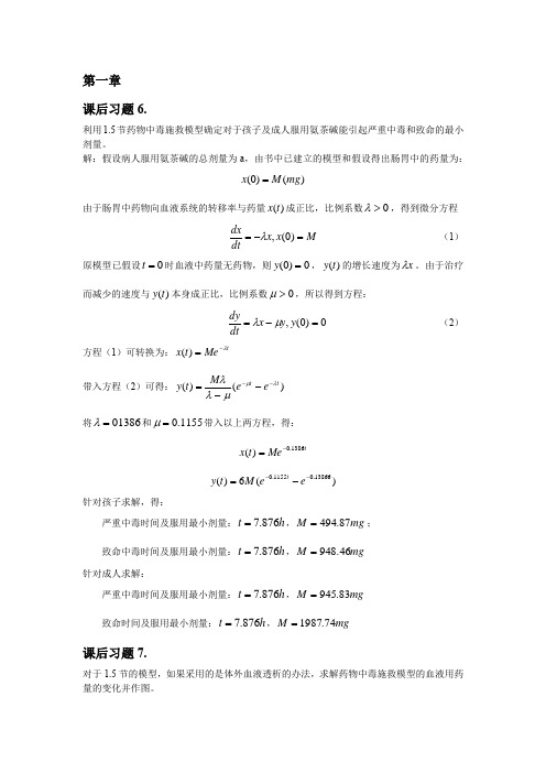
第一章 课后习题6.利用1.5节药物中毒施救模型确定对于孩子及成人服用氨茶碱能引起严重中毒和致命的最小剂量。
解:假设病人服用氨茶碱的总剂量为a ,由书中已建立的模型和假设得出肠胃中的药量为:)()0(mg M x =由于肠胃中药物向血液系统的转移率与药量)(t x 成正比,比例系数0>λ,得到微分方程M x x dtdx=-=)0(,λ (1) 原模型已假设0=t 时血液中药量无药物,则0)0(=y ,)(t y 的增长速度为x λ。
由于治疗而减少的速度与)(t y 本身成正比,比例系数0>μ,所以得到方程:0)0(,=-=y y x dtdyμλ (2) 方程(1)可转换为:tMe t x λ-=)(带入方程(2)可得:)()(t t e e M t y λμμλλ----=将01386=λ和1155.0=μ带入以上两方程,得:t Me t x 1386.0)(-= )(6)(13866.01155.0---=e e M t y t针对孩子求解,得:严重中毒时间及服用最小剂量:h t 876.7=,mg M 87.494=; 致命中毒时间及服用最小剂量:h t 876.7=,mg M 8.4694= 针对成人求解:严重中毒时间及服用最小剂量:h t 876.7=,mg M 83.945= 致命时间及服用最小剂量:h t 876.7=,mg M 74.1987=课后习题7.对于1.5节的模型,如果采用的是体外血液透析的办法,求解药物中毒施救模型的血液用药量的变化并作图。
解:已知血液透析法是自身排除率的6倍,所以639.06==μut e t x λ-=1100)(,x 为胃肠道中的药量,1386.0=λ )(6600)(t t e e t y λμ---=1386.0,639.0,5.236)2(,1100,2,====≥-=-λλλu z e x t uz x dtdzt 解得:()2,274.112275693.01386.0≥+=--t e e t z t t用matlab 画图:图中绿色线条代表采用体外血液透析血液中药物浓度的变化情况。
数学建模 建模答案.docx

programi :(1) function [accum, varargout] = CircularHough_Grd(img, radrange, varargin) %Detect circular shapes in a grayscale image. Resolve their center %positions and radii.%% [accum, circen, cirrad, dbg_LMmask] = CircularHough_Grd(% img, radrange, grdthres, fltr4LM_R, multirad, fltr4accum)% Circular Hough transform based on the gradient field of an image.% NOTE: Operates on grayscale images, NOT B/W bitmaps.% NO loops in the implementation of Circular Hough transform,% which means faster operation but at the same time larger% memory consumption.%%%%%%%%% INPUT: (img, radrange, grdthres, fltr4LM_R, multirad, fltr4accum) % % img: A 2-D grayscale image (NO B/W bitmap)%% radrange: The possible minimum and maximum radii of the circles% to be searched, in the format of% [minimum radius , maximum_radius] (unit: pixels)% **NOTE**: A smaller range saves computational time and% memory.%% grdthres: (Optional, default is 10, must be non-negative)% The algorithm is based on the gradient field of the% input image. A thresholding on the gradient magnitude% is performed before the voting process of the Circular% Hough transform to remove the Uniform intensity'% (sort-of) image background from the voting process.% In other words, pixels with gradient magnitudes smaller% than 'grdthres' are NOT considered in the computation.% **NOTE**: The default parameter value is chosen for% images with a maximum intensity close to 255. For cases% with dramatically different maximum intensities, e.g.% 10-bit bitmaps in stead of the assumed 8-bit, the default% value can NOT be used. A value of 4% to 10% of the maximum% intensity may work for general cases.%% fltr4LM_R: (Optional, default is 8, minimum is 3)% The radius of the filter used in the search of local% maxima in the accumulation array. To detect circles whose% shapes are less perfect, the radius of the filter needs% to be set larger.%% multirad: (Optional, default is 0.5)% In case of concentric circles, multiple radii may be% detected corresponding to a single center position. This% argument sets the tolerance of picking up the likely% radii values. It ranges from 0.1 to 1, where 0.1% corresponds to the largest tolerance, meaning more radii % values will be detected, and 1 corresponds to the smallest % tolerance, in which case only the "principal" radius will% be picked up.%% fltr4accum: (Optional. A default filter will be used if not given)% Filter used to smooth the accumulation array. Depending % on the image and the parameter settings, the accumulation % array built has different noise level and noise pattern% (e.g. noise frequencies). The filter should be set to an% appropriately size such that ifs able to suppress the% dominant noise frequency.%%%%%%%%% OUTPUT: [accum, circen, cirrad, dbg_LMmask]%% accum: The result accumulation array from the Circular Hough% transform. The accumulation array has the same dimension % as the input image.%% circen: (Optional)% Center positions of the circles detected. Is a N-by-2% matrix with each row contains the (x, y) positions% of a circle. For concentric circles (with the same center% position), say k of them, the same center position will% appear k times in the matrix.%% cirrad: (Optional)% Estimated radii of the circles detected. Is a N-by-1% column vector with a one-to-one correspondance to the% output tircen*. A value 0 for the radius indicates a% failed detection of the circle's radius.%% dbg_LMmask: (Optional, for debugging purpose)% Mask from the search of local maxima in the accumulation % array.%%%%%%%%%% EXAMPLE #0:% rawimg = imread('TestImg_CHT_a2.bmp');% tic;% [accum, circen, cirrad] = CircularHough_Grd(rawimg, [15 60]);% toe;% figure(l); imagesc(accum); axis image;% title(,Accumulation Array from Circular Hough Transfbrm,);% figure(2); imagesc(rawimg); colormap(,gray,); axis image;% hold on;% plot(circen(:,l), circen(:,2), *r+');% for k = 1 : size(circen, 1),% DrawCircle(circen(k, 1), circen(k,2), cirrad(k), 32,,b」);% end% hold off;% title([*Raw Image with Circles Detected% '(center positions and radii marked)*]);% figure(3); surf(accum, 'EdgeColoF, hone'); axis ij;% title('3-D View of the Accumulation Array*);%% COMMENTS ON EXAMPLE #0:% Kind of an easy case to handle. To detect circles in the image whose% radii range from 15 to 60. Default values for arguments 'grdthres',% 'fltr4LM_R', 'multirad* and ,fltr4accum, are used.%%%%%%%%%% EXAMPLE #1:% rawimg = imread('TestImg_CHT_a3.bmp');% tic;% [accum, circen, cirrad] = CircularHough_Grd(rawimg, [15 60], 10, 20);% toe;% figure(l); imagesc(accum); axis image;% title(,Accumulation Array from Circular Hough Transfbrm,);% figure(2); imagesc(rawimg); colormap('gray'); axis image;% hold on;% plot(circen(:,l), circen(:,2), T+');% for k = 1 : size(circen, 1),% DrawCircle(circen(k, 1), circen(k,2), cirrad(k), 32, 'b-');% end% hold off;% title([*Raw Image with Circles Detected% '(center positions and radii marked)*]);% figure(3); surf(accum, 'EdgeColoF, hone'); axis ij;% title(*3-D View of the Accumulation Array*);%% COMMENTS ON EXAMPLE #1:% The shapes in the raw image are not very good circles. As a result,% the profile of the peaks in the accumulation array are kind of% 'stumpy', which can be seen clearly from the 3-D view of the% accumulation array, (As a comparison, please see the sharp peaks in % the accumulation array in example #0) To extract the peak positions % nicely, a value of 20 (default is 8) is used for argument 'fltr4LM_R', % which is the radius of the filter used in the search of peaks.%%%%%%%%%% EXAMPLE #2:% rawimg = imread(,TestImg_CHT_b3 .bmp1);% fltr4img = [1 1 1 1 1; 1 2 2 2 1; 1 2 4 2 1; 1 2 2 2 1; 1 1 1 1 1];% fltr4img = fltr4img / sum(fltr4img(:));% imgfltrd = filter2( fltr4img , rawimg );% tic;% [accum, circen, cirrad] = CircularHough_Grd(imgfltrd, [15 80], 8, 10); % toe;% figure(l); imagesc(accum); axis image;% title(,Accumulation Array from Circular Hough Transfbrm,);% figure(2); imagesc(rawimg); colormap('gray'); axis image;% hold on;% plot(circen(:,l), circen(:,2), T+');% for k = 1 : size(circen, 1),% DrawCircle(circen(k, 1), circen(k,2), cirrad(k), 32, 'b-');% end% hold off;% title([*Raw Image with Circles Detected% '(center positions and radii marked)*]);%% COMMENTS ON EXAMPLE #2:% The circles in the raw image have small scale irregularities along % the edges, which could lead to an accumulation array that is bad for % local maxima detection. A 5-by-5 filter is used to smooth out the % small scale irregularities. A blurred image is actually good for the % algorithm implemented here which is based on the image's gradient % field.%%%%%%%%%% EXAMPLE #3:% rawimg = imread('TestImg_CHT_c3.bmp');% fltr4img = [1 1 1 1 1; 1 2 2 2 1; 1 2 4 2 1; 1 2 2 2 1; 1 1 1 1 1];% fltr4img = fltr4img / sum(fltr4img(:));% imgfltrd = filter2( fltr4img , rawimg );% tic;% [accum, circen, cirrad]=...% CircularHough_Grd(imgfltrd, [15 105], 8, 10, 0.7);% toe;% figure(l); imagesc(accum); axis image;% figure(2); imagesc(rawimg); colormap(,gray,); axis image;% hold on;% plot(circen(:,l), circen(:,2), *r+');% for k = 1 : size(circen, 1),% DrawCircle(circen(k, 1), circen(k,2), cirrad(k), 32,,b」);% end% hold off;% title([*Raw Image with Circles Detected% '(center positions and radii marked)*]);%% COMMENTS ON EXAMPLE #3:% Similar to example #2, a filtering before circle detection works for% noisy image too. 'multirad* is set to 0.7 to eliminate the false% detections of the circles* radii.%%%%%%%%%% BUG REPORT:% This is a beta version. Please send your bug reports, comments and% suggestions to pengtao@ . Thanks.%%%%%%%%%%% INTERNAL PARAMETERS:% The INPUT arguments are just part of the parameters that are used by% the circle detection algorithm implemented here. Variables in the code% with a prefix ,prm_, in the name are the parameters that control the% judging criteria and the behavior of the algorithm. Default values for% these parameters can hardly work for all circumstances. Therefore, at% occasions, the values of these INTERNAL PARAMETERS (parameters that% are NOT exposed as input arguments) need to be fine-tuned to make% the circle detection work as expected.% The following example shows how changing an internal parameter could% influence the detection result.% 1. Change the value of the internal parameter 'prm LM LoBndRa* to 0.4% (default is 0.2)% 2. Run the following matlab code:% fltr4accum = [1 2 1; 2 6 2; 1 2 1];% fltr4accum = fltr4accum / sum(fltr4accum(:));% rawimg = imread(,Frame_0_0022jportion.jpg,);% tic;% [accum, circen] = CircularHough_Grd(rawimg,...% [4 14], 10, 4, 0.5, fltr4accum);% toe;% figure(l); imagesc(accum); axis image;% title(*Accumulation Array from Circular Hough Transform*);% figure(2); imagesc(rawimg); colormap(,gray,); axis image;% hold on; plot(circen(:,l), circen(:,2), "); hold off;% title('Raw Image with Circles Detected (center positions marked)*);% 3. See how different values of the parameter 'prm LM LoBndRa* could % influence the result.% Author: Tao Peng% Department of Mechanical Engineering% University of Maryland, College Park, Maryland 20742, USA% pengtao@% Version: Beta Revision: Mar. 07, 2007%%%%%%%% Arguments and parameters %%%%%%%%%%%%%%%%%%%%%%%%%%%%%%%%%%%% Validation of argumentsif ndims(img)〜=2 || 〜isnumeric(img),error(*CircularHough_Grd: "img" has to be 2 dimensionaf);endif 〜all(size(img) >= 32),erro^'CircularHough Grd: "img" has to be larger than 32-by-32');endif numel(radrange)〜=2 || -isnumeric(radrange),error([*CircularHough_Grd: "radrange" has to be \ ...'a two-element vector1]);endprm_r_range = sort(max( [0,0;radrange( 1 ),radrange(2)]));% Parameters (default values)prmgrdthres = 10;prmfltrLMR = 8;prmmultirad = 0.5;funccompucen = true;funccompuradii = true;% Validation of argumentsvapgrdthres = 1;if nargin > (1 + vap_grdthres),if isnumeric(varargin{vap grdthres}) && ...varargin(vap grdthres} (1) >= 0,prm_grdthres = varargin {vapgrdthres} (1);elseerror(['CircularHough_Grd: "grdthres" has to be'a non-negative number1]);endendvap_fltr4LM = 2; % filter for the search of local maximaif nargin > (1 + vap_fltr4LM),if isnumeric(varargin{vap_fltr4LM}) && varargin{vap_fltr4LM}(1) >= 3, prmfltrLMR = varargin{vap_fltr4LM} (1);elseerror([,CircularHough_Grd: n fltr4LM_R n has to belarger than or equal to 3']);endendvap_multirad = 3;if nargin > (1 + vap multirad),if isnumeric(varargin{vap_multirad}) && ...varargin{vap multirad}(1) >= 0.1 && ...varargin {vap multirad} (1) <= 1,prmmultirad = varargin {vap_mul tirad} (1);elseerror(['CircularHough_Grd: "multirad" has to be'within the range [0.1, 1]*]);endendvap_fltr4accum = 4; % filter for smoothing the accumulation arrayif nargin > (1 + vap_fltr4accum),if isnumeric(varargin{vap_fltr4accum}) && ...ndims(varargin{vap_fltr4accum}) == 2 && ...all(size(varargin {vap_fltr4accum}) >= 3),fltr4accum = varargin {vap_fltr4accum};elseerror(['CircularHough_Grd: n fltr4accum n has to be \ ...*a 2-D matrix with a minimum size of 3-by-3']);endelse% Default filter (5-by-5)fltr4accum = ones(5,5);fltr4accum(2:4,2:4) = 2;fltr4accum(3,3) = 6;end func_compu_cen = (nargout > 1 );func_compu_radii = (nargout > 2 );% Reserved parametersdbg on = false; % debug information dbgbfigno = 4;if nargout > 3, dbg on = true; end%%%%%%%% Buildingaccumulation array %%%%%%%%%%%%%%%%%%%%%%%%%%%%%%%%% Convert the image to single if it is not of% class float (single or double) img_is_double = isa(img, double');if ~(img_is_double || isa(img, 'single')),imgf = single(img);end% Compute the gradient and the magnitude of gradientif img_is_double,[grdx, grdy] = gradient(img);else[grdx, grdy] = gradient(imgf);endgrdmag = sqrt(grdx.A2 + grdy.A2);% Get the linear indices, as well as the subscripts, of the pixels% whose gradient magnitudes are larger than the given threshold grdmasklin = find(grdmag > prm_grdthres);[grdmask_ldxl, grdmask_IdxJ] = ind2sub(size(grdmag), grdmasklin);% Compute the linear indices (as well as the subscripts) of% all the votings to the accumulation array.% The Matlab function 'accumarray* accepts only double variable, % so all indices are forced into double at this point.% A row in matrix ,lin2accum_aJ, contains the J indices (into the % accumulation array) of all the votings that are introduced by a % same pixel in the image. Similarly with matrix linZaccum aP. rr_41inaccum = double( prm_r_range );linaccum_dr = [ (-rr_41inaccum(2) + 0.5) : -rr_41inaccum(l),... (rr_41inaccum(l) + 0.5) : rr_41inaccum(2)];lin2accum_aJ = floor(...double(grdx(grdmasklin)./grdmag(grdmasklin)) * linaccum_dr + ...repmat( double(grdmask_IdxJ)+0.5 , [ 1 ,length(linaccum_dr)])...);lin2accum_al = floor(...double(grdy(grdmasklin)./grdmag(grdmasklin)) * linaccum dr + ...repmat( double(grdmask_IdxI)+0.5 , [1 ,length(linaccum_dr)])...);% Clip the votings that are out of the accumulation arraymask_valid_a J al =...lin2accum_aJ > 0 & lin2accum_aJ < (size(grdmag,2) + 1) & ...Iin2accum_al > 0 & lin2accum_al < (size(grdmag,l) + 1);mask_valid_aJaI_reverse =〜mask_valid_aJaI;lin2accum_aJ = lin2accum_aJ .* maskvalida J al + maskvalidaJ alreverse;lin2accum_al = lin2accum_al .* mask_valid_aJaI + mask_valid_aJaI_reverse;clear mask_valid_aJ alre verse;% Linear indices (of the votings) into the accumulation arraylin2accum = sub2ind( size(grdmag), lin2accum_al, lin2accum_aJ );lin2accum_size = size( lin2accum );lin2accum = reshape( lin2accum, [numel(lin2accum),l]);clear lin2accum_al lin2accum_aJ;% Weights of the votings, currently using the gradient maginitudes% but in fact any scheme can be used (application dependent)weight4accum =...repmat( double(grdmag(grdmasklin)) , [lin2accum_size(2), 1 ]) .* ...mask_valid_aJ al(:);clear mask_valid_aJaI;% Build the accumulation array using Matlab function 'accumarray'accum = accumarray( lin2accum , weight4accum );accum = [ accum ; zeros( numel(grdmag) - numel(accum), 1 )];accum = reshape( accum, size(grdmag));%%%%%%%% Locating local maxima in the accumulation array %%%%%%%%%%%%% Stop if no need to locate the center positions of circlesif ~func_compu_cen,return;endclear lin2accum weight4accum;% Parameters to locate the local maxima in the accumulation array% — Segmentation of 'accum' before locating LM prmuseaoi = true;prm_aoithres_s = 2;prm aoiminsize = floor(min([ min(size(accum)) * 0.25,... prm_r_range(2) * 1.5 ]));% — Filter for searching for local maxima prmfltrLMs = 1.35;prm fltrLM r = ceil( prm fltrLM R * 0.6 );prm fltrLM npix = max([ 6, ceil((prm_fltrLM_R/2)A 1.8)]);% — Lower bound of the intensity of local maximaprm LM LoBndRa = 0.2; % minimum ratio of LM to the max of'accum'% Smooth the accumulation arrayfltr4accum = fltr4accum / sum(fltr4accum(:));accum = filter2( fltr4accum, accum );% Select a number of Areas-Of^Interest from the accumulation array if prmuseaoi, % Threshold value for 'accum1prm_llm_thresl = prm_grdthres * prm_aoithres_s;% Thresholding over the accumulation array accummask = ( accum > prm llm thres 1 );% Segmentation over the mask[accumlabel, accum nRgn] = bwlabel( accummask, 8 );% Select AOIs from segmented regionsaccumAOI = ones(0,4);for k = 1 : accum nRgn,accumrgn lin = find( accumlabel = k);[accumrgn_ldxl, accumrgn_IdxJ]=...ind2sub( size(accumlabel), accumrgn lin);rgn top = min( accumrgn ldxl);rgn bottom = max( accumrgn_ldxl);rgn left = min( accumrgn ldxJ );rgn_right = max( accumrgn ldxJ );% The AOIs selected must satisfy a minimum sizeif ((rgn_right - rgn_left + 1) >= prm_aoiminsize && ...(rgn_bottom - rgn top + 1) >= prm aoiminsize ),accumAOI = [ accumAOI;...rgn top, rgn bottom, rgn left, rgn right ];endendelse% Whole accumulation array as the one AOIaccumAOI = [1, size(accum,l), 1, size(accum,2)];end% Thresholding of 'accum' by a lower boundprm LM LoBnd = max(accum(:)) * prm LM LoBndRa;% Build the filter for searching for local maxima fltr4LM = zeros(2 * prm_fltrLM_R + 1);[mesh4fLM_x, mesh4fLM_y] = meshgrid(-prm_fltrLM_R : prm fltrLM R);mesh4fLM_r = sqrt( mesh4fLM_x.A2 + mesh4fLM_y.A2 );fltr4LM_mask =...(mesh4fLM_r > prm_fltrLM_r & mesh4fLM_r <= prm fltrLM R );fltr4LM = fltr4LMfltr4LM_mask * (prm fltrLM s / sum(fltr4LM_mask(:)));if prm_fltrLM_R >= 4,fltr4LM_mask = ( mesh4fLM_r < (prm_fltrLM_r - 1));elsefltr4LM_mask = ( mesh4fLM_r < prm fltrLM r );endfltr4LM = fltr4LM + fltr4LM mask / sum(fltr4LM_mask(:));% **** Debug code (begin)if dbg_on,dbg_LMmask = zeros(size(accum));end% **** Debug code (end)% For each of the AOIs selected, locate the local maximacircen = zeros(0,2);fbrk = 1 : size(accumAOI, 1),aoi = accumAOI(k,:); % just for referencing convenience% Thresholding of 'accum* by a lower boundaccumaoi_LBMask =...(accum(aoi(l):aoi(2), aoi(3):aoi(4)) > prm LM LoBnd );% Apply the local maxima filtercandLM = conv2( accum(aoi( 1):aoi(2), aoi(3):aoi(4)),...fltr4LM, 'same*);candLM mask = ( candLM > 0 );% Clear the margins of 'candLM mask*candLM_mask([l :prm_fltrLM_R, (end-prm_fltrLM_R+l):end], :) = 0;candLM mask(:, [l:prm_fltrLM_R, (end-prm_fltrLM_R+l):end]) = 0;% **** Debug code (begin)if dbg_on,dbg_LMmask(aoi( 1 ):aoi(2), aoi(3):aoi(4))=...dbg_LMmask(aoi( 1 ):aoi(2), aoi(3):aoi(4)) + ...accumaoi LBMask + 2 * candLM mask;end% **** Debug code (end)% Group the local maxima candidates by adjacency, compute the% centroid position for each group and take that as the center% of one circle detected[candLM label, candLM nRgn] = bwlabel( candLM_mask, 8 );fbr ilabel = 1 : candLM nRgn,% Indices (to current AOI) of the pixels in the groupcandgrp masklin = find( candLM label == ilabel);[candgrp_ldxl, candgrp_IdxJ]=...ind2sub( size(candLM label), candgrp masklin );% Indices (to 'accum') of the pixels in the groupcandgrp_ldxl = candgrp_ldxl + ( aoi(l) - 1 );candgrp IdxJ = candgrp IdxJ + ( aoi(3) - 1 );candgrp_idx2acm =...sub2ind( size(accum) , candgrp ldxl, candgrp IdxJ );% Minimum number of qulified pixels in the groupif sum(accumaoi_LBMask(candgrp_masklin)) < prm_fltrLM_npix, continue;end% Compute the centroid positioncandgrp_acmsum = sum( accum(candgrp_idx2acm));cc_x = sum( candgrp IdxJ .* accum(candgrp_idx2acm) ) / ...candgrpacmsum;cc_y = sum( candgrp_ldxl .* accum(candgrp_idx2acm) ) / ...candgrpacmsum;circen = [circen; cc_x, cc_y];endend% **** Debug code (begin)if dbg_on,figure(dbg bfigno); imagesc(dbg LMmask); axis image;title(*Generated map of local maxima1);if size(accumAOI, 1) == 1,figure(dbg_bfigno+1);surf(candLM, 'EdgeColor1, hone'); axis ij;title(,Accumulation array after local maximum filtering*);endend% **** Debug code (end)%%%%%%%% Estimation of the Radii of Circles %%%%%%%%%%%%% Stop if no need to estimate the radii of circlesif ~func_compu_radii,varargout{l} = circen;return;end% Parameters for the estimation of the radii of circlesfltr4SgnCv=[2 1 1];fltr4SgnCv = fltr4SgnCv / sum(fltr4SgnCv);% Find circle's radius using its signature curve cirrad = zeros( size(circen,l), 1 );for k = 1 : size(circen,l),% Neighborhood region of the circle for building the sgn. curve circen_round = round( circen(k,:));SCvR IO = circen_round(2) - prm_r_range(2) - 1;ifSCvR_IO<l,SCvR_I0= 1;endSCvRIl = circen_round(2) + prm_r_range(2) + 1;if SCvR Il > size(grdx,l),SCvRIl = size(grdx,l);endSCvR JO = circen round(l) - prm_r_range(2) - 1;ifSCvR_JO<l,SCvRJO = 1;endSCvRJ 1 = circenround(l) + prm_r_range(2) + 1;if SCvR Jl > size(grdx,2),SCvRJl = size(grdx,2);end% Build the sgn. curveSgnCvMat_dx = repmat( (SCvR J0:SCvR J 1) - circen(k,l),...[SCvRJl - SCvRJO +1,1]);SgnCvMat_dy = repmat( (SCvR_IO:SCvR_Il)' - circen(k,2),...[1 , SCvRJl - SCvRJO + 1]);SgnCvMat_r = sqrt( SgnCvMat dx .A2 + SgnCvMat_dy .A2 );SgnCvMatrpl = round(SgnCvMatr) + 1;f4SgnCv = abs(...double(grdx(SCvR_IO:SCvR_Il, SCvRJO:SCvRJ 1)) .* SgnCvMat_dx + ...double(grdy(SCvR_IO:SCvR Il, SCvR JO:SCvR J 1)) .* SgnCvMat dy...)./ SgnCvMat r;SgnCv = accumarray( SgnCvMat rp 1(:) , f4SgnCv(:));SgnCv_Cnt = accumarray( SgnCvMat rp 1 (:) , ones(numel(f4SgnCv), 1));SgnCv_Cnt = SgnCv_Cnt + (SgnCv_Cnt == 0);SgnCv = SgnCv ./ SgnCv_Cnt;% Suppress the undesired entries in the sgn. curve% ― Radii that correspond to short arcsSgnCv = SgnCv .* ( SgnCv_Cnt >= (pi/4 * [O:(numel(SgnCv_Cnt)-1 )]*));% ― Radii that are out of the given rangeSgnCv( 1 : (round(prm_r_range( 1))+1) ) = 0;SgnCv( (round(prm_r_range(2))+1) : end ) = 0;% Get rid of the zero radius entry in the arraySgnCv = SgnCv(2:end);% Smooth the sgn. curveSgnCv = filtfilt( fltr4SgnCv , [1] , SgnCv );% Get the maximum value in the sgn. curveSgnCv_max = max(SgnCv);if SgnCv_max <= 0,cirrad(k) = 0;continue;end% Find the local maxima in sgn. curve by 1st order derivatives% ― Mark the ascending edges in the sgn. curve as Is and% ― descending edges as OsSgnCv AscEdg = ( SgnCv(2:end) - SgnCv(l:(end-l)) ) > 0;% ― Mark the transition (ascending to descending) regionsSgnCv LMmask = [ 0; 0; SgnCv_AscEdg(l:(end-2)) ] & (〜SgnCv_AscEdg);SgnCv LMmask = SgnCvLMmask & [ SgnCv_LMmask(2:end); 0 ];% Incorporate the minimum value requirementSgnCvLMmask = SgnCvLMmask & ...(SgnCv(l:(end-l)) >= (prm_multirad * SgnCv_max));% Get the positions of the peaksSgnCv LMPos = sort( find(SgnCv_LMmask));% Save the detected radiiif isempty(SgnCvLMPos),cirrad(k) = 0;elsecirrad(k) = SgnCvLMPos(end);for i radii = (length(SgnCv LMPos) - 1) : -1 : 1,circen = [ circen; circen(k,:)];cirrad = [ cirrad; SgnCv_LMPos(i_radii)];endendend% Outputvarargout{l} = circen;varargout{2} = cirrad;if nargout > 3,varargout{3} = dbg_LMmask;endprograms:programs:2 function DrawCircle (x, y, r, nseg, S)% Draw a circle on the current figure using ploylines%% DrawCircle (x, y, r, nseg, S)% A simple function for drawing a circle on graph.%% INPUT: (x, y, r, nseg, S)% x, y: Center of the circle% r: Radius of the circle% nseg: Number of segments for the circle% S: Colors, plot symbols and line types%% OUTPUT: None%% BUG REPORT:% Please send your bug reports, comments and suggestions to% pengtao@glue. umd. edu . Thanks.% Author: Tao Peng% Department of Mechanical Engineering% University of Maryland, College Park, Maryland 20742, USA % pengtao@glue. umd. edu% Version: alpha Revision: Jan. 10, 2006theta = 0 : (2 * pi / nseg) : (2 * pi);pline_x 二r * cos(theta) + x;pline_y 二r * sin(theta) + y;plot (pline_x, pline_y, S);3function testiml二imread (' image 1. jpg');% rawimg = imread(,TestImg_CHT_c3. bmp J);rawimg=rgb2gray(iml);tic;[accum, circen, cirrad] = CircularHough_Grd(rawimg, [20 30], 5,50);circentoe;figure(1) ; imagesc(accum); axis image;title (J Accumulation Array from Circular Hough Transform,); figure (2) ; imagesc (rawimg) ; colormap (J gray,) ; axis image; hold on;plot (circen(:, 1), circen(:, 2), ' r+');for k = 1 : size (circen, 1),DrawCircle (circen (k, 1), circen (k, 2), cirrad (k), 32, ' b-'); end hold off; title(f Raw Image with Circles Detected ...'(center positions and radii marked)']);figure (3); surf(accum, ' EdgeColor,, ' none5); axis ij; title (J 3-D View of the Accumulation Array');附带图像image 1. jpg直接运行test.m即可得到上方的结果!当然方法是活的,只要合理即可行。
- 1、下载文档前请自行甄别文档内容的完整性,平台不提供额外的编辑、内容补充、找答案等附加服务。
- 2、"仅部分预览"的文档,不可在线预览部分如存在完整性等问题,可反馈申请退款(可完整预览的文档不适用该条件!)。
- 3、如文档侵犯您的权益,请联系客服反馈,我们会尽快为您处理(人工客服工作时间:9:00-18:30)。
于是每天的平均费用是
(3)
模型求解:求 使(3)式的 最小。容易得到 (4)代入(1)式可得
由(3)式算出最小的总费用为
\
500元以上1224%
手工艺品,它运用不同的材料,通过不同的方式,经过自己亲手动手制作。看着自己亲自完成的作品时,感觉很不同哦。不论是01年的丝带编织风铃,02年的管织幸运星,03年的十字绣,04年的星座手链,还是今年风靡一时的针织围巾等这些手工艺品都是陪伴女生长大的象征。为此,这些多样化的作品制作对我们这一创业项目的今后的操作具有很大的启发作用。
2、原型:原型指人们在现实世界里关心、研究或者从事生产、管理的实际对象。
3、机理分析:根据对客观事物特性的认识,找出反映内部机理的数量规律,建立的模型常有明显的物理意义或现实意义。
4、概率模型:如何用随机变量和概率分布描述随机因素的影响,建立比较简单的随机模型叫概率模型。
5、
二、填空题
1、描述模型、预报模型、优化模型、决策模型、控制模型
2、每次生产准备费为 ,每天每件产品贮存费为 ;
3、生产能力为无限大(相对于需求量),当贮存量降到零时, 件产品立即生产出来供给需求,即不允许缺货。
模型建立:将贮存量表示为时间 的函数 , 生产 件,贮存量 , 以需求速率 递减,直到 ,如图1。显然有
(1)
图1不允许缺货模型的贮存量
一个周期内的贮存费是 ,其中积分恰等于图1中三角形A的面积 。因为一周期的准备费是 ,再注意到(1)式,得到一周期的总费用为
(1)专业知识限制
3、答:(1)列出约束条件及目标函数(2)画出约束条件所表示的可行域(3)在可行域内求目标函数的最优解及最优值。
4、答:随机存储策略是反映存储策略(库存数题
1、答:题涉及到时间、地点和人员三大因素,故应该考虑到的因素至少有以下几个:
(1)教师:是否连续上课,对时间的要求,对多媒体的要求和课程种类的限制等;
西南大学网络与继续教育学院课程考试答题卷
学号:1517580663001姓名:任文莉2016年6月
课程名称【编号】:数学建模【0349】
(横线以下为答题区)
答题不需复制题目,写明题目编号,按题目顺序答题
一、名词解释
1、数学模型:是由数字、字母或其它数字符号组成的,描述现实对象数量规律的数学公式、图形或算法。
五、计算题
1、解:人口净增长率与人口极限以及目前人口均相关。人口量的极限为M,当前人口数量为N(t),r为比例系数。建立模型:
求解得到
注意到当N(t) 时, 并说明r即为自然增长率。
2、解:模型假设:为了处理的方便,考虑连续模型,即设生产周期 和产量 均为连
量。根据问题性质作如下假设:
1、产品每天的需求量为常数 ;
“碧芝自制饰品店”拥有丰富的不可替代的异国风采和吸引人的魅力,理由是如此的简单:世界是每一个国家和民族都有自己的饰品文化,将其汇集进行再组合可以无穷繁衍。
1996年“碧芝自制饰品店”在迪美购物中心开张,这里地理位置十分优越,交通四通八达,由于位于市中心,汇集了来自各地的游客和时尚人群,不用担心客流量的问题。迪美有300多家商铺,不包括柜台,现在这个商铺的位置还是比较合适的,位于中心地带,左边出口的自动扶梯直接通向地面,从正对着的旋转式楼梯阶而上就是人民广场中央,周边4、5条地下通道都交汇于此,从自家店铺门口经过的90%的顾客会因为好奇而进去看一下。
2、X(t)=rX(1-X/N)
3、随机变量、概率分布
4、19.44万元
5、19天,2090件
6、想象和逻辑思维
三、问答题
1、答(1)在一般工程技术领域,数学建模仍然大有用武之地。
(2)在高新技术领域,数学建模几乎是必不可少的工具。
(3)数学迅速进入一些新领域,为数学建模开拓了许多新的处女地。
2、答:确定性模型和随机性模型、静态模型和动态模型、线性模型和非线性模型、离散模型和连续模型。
“碧芝”最吸引人的是那些小巧的珠子、亮片等,都是平日里不常见的。店长梁小姐介绍,店内的饰珠有威尼斯印第安的玻璃珠、秘鲁的陶珠、奥利的施华洛世奇水晶、法国的仿金片、日本的梦幻珠等,五彩缤纷,流光异彩。按照饰珠的质地可分为玻璃、骨质、角质、陶制、水晶、仿金、木制等种类,其造型更是千姿百态:珠型、圆柱型、动物造型、多边形、图腾形象等,美不胜收。全部都是进口的,从几毛钱一个到几十元一个的珠子,做一个成品饰物大约需要几十元,当然,还要决定于你的心意。“碧芝”提倡自己制作:端个特制的盘子到柜台前,按自己的构思选取喜爱的饰珠和配件,再把它们串成成品。这里的饰珠和配件的价格随质地而各有同,所用的线绳价格从几元到一二十元不等,如果让店员帮忙串制,还要收取10%~20%的手工费。
上海市劳动和社会保障局所辖的“促进就业基金”,还专门为大学生创业提供担保,贷款最高上限达到5万元。
调研要解决的问题:
2、消费者分析
大学生的消费是多种多样,丰富多彩的。除食品外,很大一部分开支都用于。服饰,娱乐,小饰品等。女生都比较偏爱小饰品之类的消费。女生天性爱美,对小饰品爱不释手,因为饰品所展现的魅力,女人因饰品而妩媚动人,亮丽。据美国商务部调查资料显示女人占据消费市场最大分额,随社会越发展,物质越丰富,女性的时尚美丽消费也越来越激烈。因此也为饰品业创造了无限的商机。据调查统计,有50%的同学曾经购买过DIY饰品,有90%的同学表示若在学校附近开设一家DIY手工艺制品,会去光顾。我们认为:我校区的女生就占了80%。相信开饰品店也是个不错的创业方针。
(2)学生:是否连续上课,专业课课时与共同课是否冲突,选修人数等;
(3)教室:教室的数量,教室的容纳量,是否具备必要的多媒体等条件;
2、答:(1)因为可行域的右上方无界,故将出现目标函数趋于无穷大的情形,结果是问题具有无界解;
(2)将最优解代入约束条件可知第二个约束条件为严格不等式,而其他为严格等式。这说明,铁和钙的摄入量达标,而蛋白质的摄入量超最低标准18个单位。