搅拌摩擦焊的工艺参数
搅拌摩擦加工(FSP)介绍

1 搅拌摩擦加工(FSP)简介
Fig 5. Macrostructure of dissimilar joints: (a) 1000-40, (b) 1000120, (c) 1000-240 and the corresponding surfaces (d-f)
搅拌摩擦加工(FSP)是在搅拌摩擦焊 (FSW)的基础上发展而来的一种加工技术。
图4 航天特焊无倾角搅拌头
图3 搅拌摩擦加工(FSP) 主要工艺参数
1 搅拌摩擦加工(FSP)简介
Fห้องสมุดไป่ตู้P原理——利用搅拌头剧烈的搅拌作用,造成加工区材料发生剧烈塑性变形、混 合、破碎和热暴露,实现材料微观组织的细化、均匀化和致密化
2 搅拌摩擦加工(FSP)研究
2.1.2 细晶超塑性材料制备(Mishra等)
超塑性一般大于200% 480℃时,7075-T651铝合金
最大延伸率为1250%
图9 FSP加工后的7075-T651铝合金晶粒<3.8μm
2 搅拌摩擦加工(FSP)研究
2.1.2 细晶超塑性材料制备(张大童等)
搅拌摩擦加工
Friction Stir Processing
目录
Contents
搅拌摩擦加工(FSP)简介 搅拌摩擦加工(FSP)研究 搅拌摩擦加工(FSP)特点 搅拌摩擦加工(FSP)展望
1 搅拌摩擦加工(FSP)简介
1997年,搅拌摩擦 技术被日本公司广 泛的应用于铝合金 车体制造
2002年,搅拌摩擦 焊中心在中国成立, 并在中国大力推广
δ5 ↑ 151.4%
2.1 铸造金属微观组织细化(Yaobin Wang等) 晶粒细化、消除内部缺陷
搅拌摩擦焊的原理、工艺特点、装备特点及飞机制造中的应用
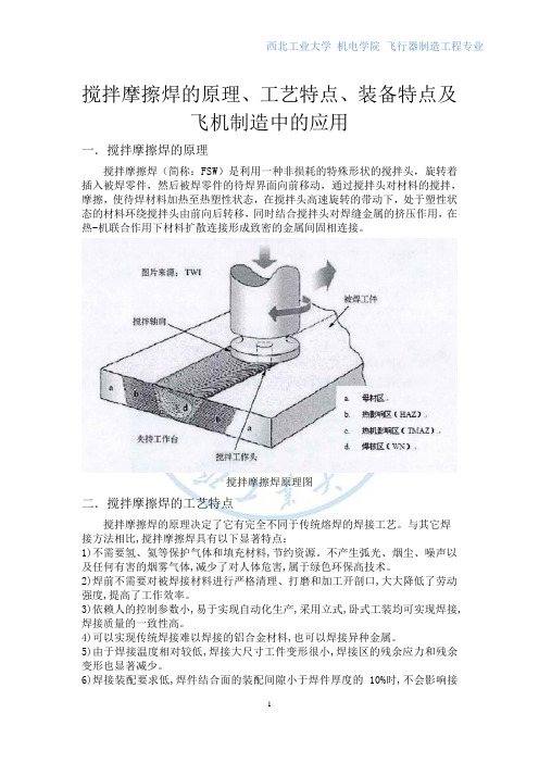
搅拌摩擦焊的原理、工艺特点、装备特点及飞机制造中的应用一.搅拌摩擦焊的原理搅拌摩擦焊(简称:FSW)是利用一种非损耗的特殊形状的搅拌头,旋转着插入被焊零件,然后被焊零件的待焊界面向前移动,通过搅拌头对材料的搅拌,摩擦,使待焊材料加热至热塑性状态,在搅拌头高速旋转的带动下,处于塑性状态的材料环绕搅拌头由前向后转移,同时结合搅拌头对焊缝金属的挤压作用,在热-机联合作用下材料扩散连接形成致密的金属间固相连接。
搅拌摩擦焊原理图二.搅拌摩擦焊的工艺特点搅拌摩擦焊的原理决定了它有完全不同于传统熔焊的焊接工艺。
与其它焊接方法相比,搅拌摩擦焊具有以下显著特点:1)不需要氢、氦等保护气体和填充材料,节约资源。
不产生弧光、烟尘、噪声以及任何有害的烟雾气体,减少了对人体危害,属于绿色环保高技术。
2)焊前不需要对被焊接材料进行严格清理、打磨和加工开剖口,大大降低了劳动强度,提高了工作效率。
3)依赖人的控制参数小,易于实现自动化生产,采用立式,卧式工装均可实现焊接,焊接质量的一致性高。
4)可以实现传统焊接难以焊接的铝合金材料,也可以焊接异种金属。
5)由于焊接温度相对较低,焊接大尺寸工件变形很小,焊接区的残余应力和残余变形也显著减少。
6)焊接装配要求低,焊件结合面的装配间隙小于焊件厚度的10%时,不会影响接头质量。
FSW技术的主要工艺参数是摩擦速度及时间,关键技术问题在于特殊结构形状的搅拌头。
对于不同的待焊材料,接头形式,搅拌头的材料和形状及搅拌摩擦焊的工艺都应不同。
三.搅拌摩擦焊的装备特点搅拌摩擦焊的搅拌头由特殊形状的搅拌指棒和轴肩组成,轴肩的直径大于搅拌指棒的直径,在焊接过程中轴肩和被焊材料的表面紧密接触,防止塑化金属材料的挤出和氧化。
同时,搅拌轴肩还可以提供部分焊接所需要的搅拌摩擦热,搅拌指棒的形状比较特殊,焊接过程中搅拌指棒要旋转着插入被焊材料的结合界面处,并且沿着待焊界面向前移动。
对于对接焊缝,搅拌指棒的插入深度一般要略小于被焊材料的厚度。
铝合金搅拌摩擦焊工艺
铝合金搅拌摩擦焊工艺铝合金搅拌摩擦焊是一种先进的焊接技术,具有高效、节能、环保等优点。
本文将详细介绍铝合金搅拌摩擦焊工艺的各个环节,帮助读者更好地了解这一技术。
一、焊接准备在进行铝合金搅拌摩擦焊之前,需要进行充分的焊接准备。
这包括检查工件表面的油污、锈迹等杂质,确保工件表面干净整洁。
同时,需要准备好搅拌头、焊机、夹具等焊接工具,并对工具进行必要的检查和调整。
二、装配铝合金搅拌摩擦焊的装配过程需要严格按照工艺要求进行。
首先,要将工件放置在夹具中,确保工件的位置和角度正确。
然后,根据焊接工艺要求,选择合适的搅拌头,并将其插入到工件中。
在装配过程中,需要保证搅拌头的稳定性和准确性,避免出现偏移或倾斜现象。
三、搅拌头插入搅拌头的插入是铝合金搅拌摩擦焊的关键步骤之一。
在插入过程中,需要控制好搅拌头的插入深度和角度,确保其与工件表面紧密贴合。
同时,要避免搅拌头与工件表面产生过大的摩擦力,以免造成工件表面损伤或搅拌头损坏。
四、搅拌摩擦在进行搅拌摩擦时,需要控制好搅拌头的旋转速度和压力,使焊缝处的材料充分流动和混合。
同时,要控制好焊接温度,避免出现过热或冷却不均匀现象。
在搅拌摩擦过程中,还需要注意搅拌头的磨损情况,及时更换磨损严重的搅拌头。
五、焊接过程控制铝合金搅拌摩擦焊的过程控制是保证焊接质量的关键。
在焊接过程中,需要实时监测焊接温度、压力、旋转速度等参数,并根据实际情况进行调整。
同时,要严格控制焊接时间,确保焊缝处的材料充分熔化和混合。
在焊接过程中,还需要注意防止外部因素对焊接质量的影响,如振动、污染等。
六、焊后处理铝合金搅拌摩擦焊完成后,需要进行必要的焊后处理。
这包括对焊缝进行冷却、去除焊渣、对焊缝进行修整等。
在冷却过程中,要控制好冷却时间和方式,避免出现裂纹等现象。
同时,需要去除焊缝表面的焊渣和氧化物,修整焊缝的形状和尺寸,使其符合工艺要求。
七、质量检测质量检测是保证铝合金搅拌摩擦焊接质量的必要环节。
检测内容包括外观检测、无损检测、力学性能检测等。
搅拌摩擦焊工艺参数
搅拌摩擦焊工艺参数
搅拌摩擦焊技术作为一种新兴的焊接方式,由于其低热输入、无
污染、高强度等特点,受到越来越多的关注和应用。
而搅拌摩擦焊工
艺参数的选择,对焊接质量和效率至关重要。
一、工艺参数的种类
搅拌摩擦焊工艺参数主要包括预压力、搅拌头形状和转速、焊接速度、钨极压力、焊接时间等几个方面。
二、主要参数的选择
1、预压力:预压力的大小对焊接接头起到重要作用。
过大的预压力会
导致变形过大,而过小则会导致压接牢固不良。
通常,预压力的大小
应是焊接接头厚度的1.5~2倍。
2、搅拌头形状和转速:搅拌头形状和转速直接影响到焊接接头
的细小高低起伏。
一般搅拌头直径应该是焊接接头厚度的1/2~3/4,而转速则要根据不同的焊接材料来选择。
3、焊接速度:焊接速度的快慢会影响焊接区域的温度分布,从
而影响到焊接接头质量。
与传统气焊相比,搅拌摩擦焊接速度通常较快,从而大大提高了生产效率。
4、钨极压力:在搅拌摩擦焊过程中,钨极压力的大小直接影响
到焊接质量。
通常,钨极压力的大小应该是焊接接头的1.5~2倍。
5、焊接时间:焊接时间是影响焊接接头质量和工艺参数选择的
一个重要参数。
一般来说,焊接时间过长不仅会导致焊接接头表面温
度过高,而且会影响焊接材料的PH值。
三、总结
综上所述,搅拌摩擦焊工艺参数的选择对焊接质量和效率有着至关重
要的作用,因此在实际应用中必须根据不同的焊接要求,综合考虑各
项参数,确定合适的工艺参数,以确保焊接接头的合格率和工艺效率。
4mm 1050 搅拌摩擦焊焊接工艺 (4)
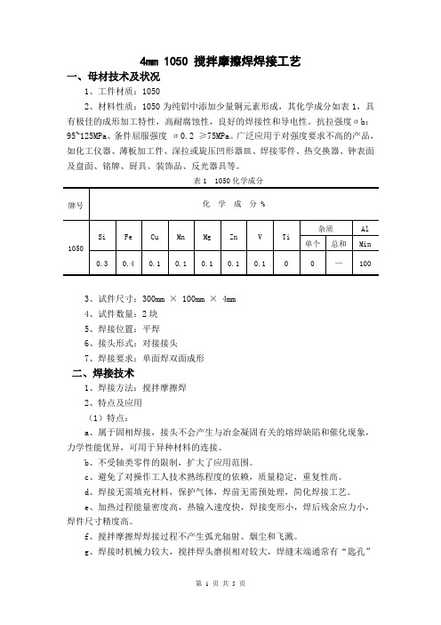
4mm 1050 搅拌摩擦焊焊接工艺一、母材技术及状况1、工件材质:10502、材料性质:1050为纯铝中添加少量铜元素形成,其化学成分如表1,具有极佳的成形加工特性,高耐腐蚀性,良好的焊接性和导电性。
抗拉强度σb:95~125MPa、条件屈服强度σ0.2 ≥75MPa。
广泛应用于对强度要求不高的产品,如化工仪器、薄板加工件、深拉或旋压凹形器皿、焊接零件、热交换器、钟表面及盘面、铭牌、厨具、装饰品、反光器具等。
表1 1050化学成分牌号化学成分 %1050Si Fe Cu Mn Mg Zn V Ti杂质Al单个总和Min 0.3 0.4 0.1 0.1 0.1 0.1 0.1 0 0 —1003、试件尺寸:300mm × 100mm × 4mm4、试件数量:2块5、焊接位置:平焊6、接头形式:对接接头7、焊接要求:单面焊双面成形二、焊接技术1、焊接方法:搅拌摩擦焊2、特点及应用(1)特点:a、属于固相焊接,接头不会产生与冶金凝固有关的熔焊缺陷和催化现象,力学性能优异,可用于异种材料的连接。
b、不受轴类零件的限制,扩大了应用范围。
c、避免了对操作工人技术熟练程度的依赖,质量稳定,重复性高。
d、焊接无需填充材料,保护气体,焊前无需预处理,简化焊接工艺。
e、加热过程能量密度高,热输入速度快,焊接变形小,焊后残余应力小,焊件尺寸精度高。
f、搅拌摩擦焊焊接过程不产生弧光辐射、烟尘和飞溅。
g、焊接时机械力较大,搅拌焊头磨损相对较大,焊缝末端通常有“匙孔”存在。
(2)应用:搅拌摩擦焊广泛应用于航天制造、飞机制造、船舶制造、轨道交通领域、汽车制造及其他工业中。
三、焊接设备及工具1、焊接设备:搅拌摩擦焊焊机,如图1所示。
如图1 搅拌摩擦焊焊机2、焊接工具:搅拌焊头,如图2所示。
如图2 搅拌焊头四、焊前准备1、坡口形式:采用“I”形坡口。
2、加工方法:可采用机械切割、等离子弧切割、碳弧气刨等方法进行坡口加工。
搅拌摩擦焊工艺参数
搅拌摩擦焊工艺参数
佚名
【期刊名称】《现代焊接》
【年(卷),期】2006(000)009
【摘要】搅拌摩擦焊工艺参数主要有搅拌头的倾角、搅拌头的旋转速度、搅拌头的插入深度、插入速度、插入停留时间、焊接速度、焊接压力、回抽停留时间、搅拌头的回抽速度等。
搅拌摩擦焊时,搅拌头通常会向前倾斜一定角度,以便焊接时搅拌头肩部的后沿能够对焊缝施加一定的焊接顶锻力。
搅拌头的倾角设计指标一般为±5°,1搅拌头倾角对于薄板(厚度为1 ̄6mm)搅拌头倾角采用小角度,通常为1 ̄2°,对于中厚板(厚度大于6mm),根据被焊接工件的结构和焊接压力的大小,搅拌头的倾角通常采用3 ̄5°。
搅拌头的旋转速度与焊接速度相关,但通常由被焊接材料的特性决定,对于特定的材料,搅拌头的旋转速度一般对应着一个最佳工艺窗口,在此窗口内旋转速度可以在一定的范围内波动,以便2搅拌头的旋转速度和焊接速度相匹配,实现高质量的焊接。
据搅拌头的旋转速度,搅拌摩擦焊接可以分为冷规范、弱规范和强规范,各种铝合材料焊接规范分类如表1所示。
搅拌头的插入深度一般指搅拌针插入被焊接材料的深度,但有时可以指搅拌肩的后沿低于板材表面的深度。
对接焊时,焊接深度一般等于搅拌针的长度,由于搅拌针的顶端距离底部3搅拌头插入深度搅拌摩擦焊专栏TheFSW Column24现代焊接2006年第...
【总页数】2页(P)
【正文语种】中文
【中图分类】TG453.9
因版权原因,仅展示原文概要,查看原文内容请购买。
铝合金搅拌摩擦焊
1自然时效 室温放置96h,
2人工时效185~195℃保温 6~12小时,空冷
分级时效:
第一步:100~130℃保温1-4h, 形成GP区 第二步:185~195℃时效8-9h,析出沉淀相
分级时效的优点:
先在一个较低的温度获得 高浓度 G.P. 区,然后再较高的温 度下获得 均匀的沉淀相, 提高组织的均匀性。
参考文献
[1]李生朋. 铝合金薄板搅拌摩擦焊焊接变形机理与控制 [D]. 中南大学, 2011.
[2]李兵 . 6063铝合金薄板搅拌摩擦焊接工艺及机理的研究 [D].东北大学, 2009. [3]胡尊艳. 焊后时效对6061-T6铝合金搅拌摩擦焊接头组织 和性能的影响[D].北京交通大学, 2008.
热影响区 : 温度不足以使沉淀相溶解,沉淀相发生粗 化。 热机械影响区:温度达到固溶温度,部分沉淀相粗化, 部分溶解,在后续的冷却过程中有少量细小沉淀析出 中心
焊核区:沉淀相完全溶解, 冷却过程中,沉淀相优 先在位错和晶界处析出,分布不均匀
五、解决方案
焊缝后续热处理 一 二 三 350~370℃保温30到120min 去应力退火 固溶处理 :加热到490~505℃, 然后水冷。 时效 :
[4]周德生. 铝合金搅拌摩擦焊构件时效成形研究[D]. 南昌 航空大学, 2011.
[5]王海艳. 6061铝合金搅拌摩擦焊接头组织和性能研究 [D]. 华南理工大学, 2010.
一、背景介绍
铝合金焊接性:
1、焊接变形 2、焊接裂纹问题 3、焊接接头软化 4、气孔
与传统熔化焊接方法相比,搅拌摩擦焊具有接头宏观形 貌良好、焊后残余应力和变形较小、焊缝性能良好;焊接 时无烟尘、无辐射;焊接过程中不需焊丝填充、不需气体 保护,比较节省成本,最大程度上缓解了因热输入过大导 致的铝合金焊接接头发生的“软化”及裂纹、气孔等严重 缺陷,因此搅拌摩擦焊特别适合于铝合金的连接。
铝合金搅拌摩擦焊工艺 -回复
铝合金搅拌摩擦焊工艺-回复铝合金搅拌摩擦焊工艺- 实现材料的高质量连接引言:铝合金是一种常用的轻质金属材料,具有优良的导热性、强度和耐腐蚀性。
在制造行业中,铝合金的应用越来越广泛,但如何高效地连接铝合金成为一个关键问题。
在铝合金的焊接方法中,搅拌摩擦焊技术因其特殊的优点而备受关注。
本文将一步一步地介绍铝合金搅拌摩擦焊工艺,以及其关键步骤和优势。
第一部分:搅拌摩擦焊的原理和过程搅拌摩擦焊是一种通过搅拌和摩擦热来实现材料结合的焊接方法。
其过程中,焊接头两侧的铝合金被高速旋转的锥形工具搅拌并加热,随着摩擦的增加,金属温度升高,导致其柔韧性增加。
当达到一定的温度时,焊接头被渐渐挤压,使得金属层之间发生冷焊结合。
同时,由于搅拌的缘故,焊接头中的金属颗粒得到细化,从而提高了焊接接头的强度和密实性。
第二部分:铝合金搅拌摩擦焊工艺步骤1. 材料准备:选择合适的铝合金材料,并确保其表面清洁和无油污。
2. 设计焊接接头:确定焊接接头的几何形状和尺寸,以及焊接参数。
3. 定位和装夹:将两个要焊接的铝合金零件放置在焊接设备上,并通过合适的夹具进行固定。
4. 焊接温度和力控制:根据材料性质和焊接要求,设定合适的旋转速度和下压力。
5. 开始搅拌:启动设备,使工具开始旋转并加热焊接区域,同时向下施加一定的压力。
6. 加热和搅拌:搅拌头的高速旋转和下压力会加热金属,并使其产生塑性变形,从而实现冷焊结合。
7. 结束焊接:在达到焊接要求后,停止旋转和施加压力,留出一定的冷却时间。
8. 检测和质量控制:使用非破坏性和破坏性测试方法来检测焊接接头的质量,确保其达到要求。
第三部分:铝合金搅拌摩擦焊的优势1. 高质量:搅拌摩擦焊可以消除气孔、热裂纹等焊接缺陷,实现金属材料的高质量连接。
2. 高效率:相较于传统的焊接方法,搅拌摩擦焊不需要额外的填充材料和气体保护,节省了时间和成本。
3. 环保:搅拌摩擦焊过程中无需使用焊接剂或保护气体,减少了对环境的污染。
2524薄板搅拌摩擦焊工艺研究
2524薄板搅拌摩擦焊工艺研究2524薄板搅拌摩擦焊工艺是极具技术难点的一种焊接工艺。
它主要应用于2524薄板的搅拌摩擦焊,它具有焊接质量高、尺寸稳定等优点,能够满足薄板结构件无损组装、焊接性能满足设计要求的需求。
由此,2524薄板搅拌摩擦焊工艺成为当前焊接应用中的一种重要工艺。
2524薄板搅拌摩擦焊工艺在过去的几十年里有许多研究工作。
在此基础上,本文从2524薄板搅拌摩擦焊工艺的机理、刀具参数等方面,综合分析该工艺的技术特性,完善其技术参数设置,提出其改进方案。
2524薄板搅拌摩擦焊工艺的机理2524薄板搅拌摩擦焊工艺是利用刀具对被焊接板材产生机械振动,产生摩擦力,在摩擦力的作用下,板材之间瞬时产生热电耦合,形成接触线,使表面金属汞化,使被焊接板材之间的接触线冶炼出来,从而形成一个完整的搅拌摩擦焊接点。
2524薄板搅拌摩擦焊工艺的刀具参数2524薄板搅拌摩擦焊工艺的刀具主要有力的参数为夹持力、摩擦转矩、摩擦前压力以及摩擦角度等,其中夹持力可影响板材间的接触度,摩擦转矩可影响板材摩擦力,摩擦前压力可改善极限特性,摩擦角度也可影响摩擦力大小,摩擦前预压力主要影响摩擦前板材间隙,这些参数是影响薄板搅拌摩擦焊质量的关键参数。
2524薄板搅拌摩擦焊工艺的改进2524薄板搅拌摩擦焊工艺的改进主要以提高刀具的耐磨性、减少工艺参数的影响、优化工艺流程、提高焊接强度与抗拉强度等方面进行研究。
首先,可以通过改变刀具材质,采用高强度钛合金、高硬度钨钢等材料制作刀具,使其具有更高的耐磨性;其次,可以采用精确控制工艺参数的方法,精确控制夹持力、摩擦转矩、摩擦角度等参数,从而减少不良焊点的产生;第三,可以优化工艺流程及过程参数,确保工艺的可控性及准确性,保证最终的焊接性能;第四,可以采用铜粉、铜锡等填充材料及金属熔料补强搅拌摩擦焊接处,提高焊接强度与抗拉强度。
综上所述,2524薄板搅拌摩擦焊工艺是一种极具技术难点的焊接工艺,从机理到参数设置,都需要把握精准,才能够满足薄板结构件的无损组装,焊接性能的满足设计要求的要求。
搅拌摩擦焊工艺参数
搅拌摩擦焊工艺参数搅拌摩擦焊是一种常用的焊接工艺,它通过搅拌和摩擦的作用,在焊缝处产生高温和高压,使金属材料发生塑性变形和热扩散,从而实现焊接连接。
搅拌摩擦焊的工艺参数对焊接质量和效率起着关键作用。
本文将从搅拌速度、搅拌角度、搅拌时间和搅拌压力四个方面介绍搅拌摩擦焊的工艺参数。
一、搅拌速度搅拌速度是指在搅拌摩擦焊过程中搅拌工具的旋转速度。
搅拌速度的选择应根据被焊接材料的性质和厚度来确定。
一般情况下,搅拌速度越高,摩擦产生的热量越大,焊接温度越高,焊接质量越好。
但是,如果搅拌速度过高,可能会导致焊接接头过热,甚至烧穿。
因此,在确定搅拌速度时,需要综合考虑焊接质量和工艺效率。
二、搅拌角度搅拌角度是指搅拌工具与被焊接材料之间的夹角。
搅拌角度的选择应根据被焊接材料的性质和形状来确定。
一般情况下,搅拌角度越大,摩擦产生的热量越集中,焊接温度越高,焊接质量越好。
但是,如果搅拌角度过大,可能会导致焊接接头过热,甚至烧穿。
因此,在确定搅拌角度时,需要综合考虑焊接质量和工艺效率。
三、搅拌时间搅拌时间是指搅拌工具在焊接过程中与被焊接材料接触的时间。
搅拌时间的选择应根据被焊接材料的性质和厚度来确定。
一般情况下,搅拌时间越长,摩擦产生的热量越大,焊接温度越高,焊接质量越好。
但是,如果搅拌时间过长,可能会导致焊接接头过热,甚至烧穿。
因此,在确定搅拌时间时,需要综合考虑焊接质量和工艺效率。
四、搅拌压力搅拌压力是指搅拌工具施加在被焊接材料上的压力。
搅拌压力的选择应根据被焊接材料的性质和厚度来确定。
一般情况下,搅拌压力越大,摩擦产生的热量越大,焊接温度越高,焊接质量越好。
但是,如果搅拌压力过大,可能会导致焊接接头过热,甚至烧穿。
因此,在确定搅拌压力时,需要综合考虑焊接质量和工艺效率。
总结起来,搅拌摩擦焊的工艺参数包括搅拌速度、搅拌角度、搅拌时间和搅拌压力。
合理选择这些参数可以保证焊接质量和工艺效率。
在确定这些参数时,需要综合考虑被焊接材料的性质和厚度,并进行试验验证。
- 1、下载文档前请自行甄别文档内容的完整性,平台不提供额外的编辑、内容补充、找答案等附加服务。
- 2、"仅部分预览"的文档,不可在线预览部分如存在完整性等问题,可反馈申请退款(可完整预览的文档不适用该条件!)。
- 3、如文档侵犯您的权益,请联系客服反馈,我们会尽快为您处理(人工客服工作时间:9:00-18:30)。
Trans. Nonferrous Met. Soc. China 22(2012) 1064í1072Correlation between welding and hardening parameters offriction stir welded joints of 2017 aluminum alloyHassen BOUZAIENE, Mohamed-Ali REZGUI, Mahfoudh AYADI, Ali ZGHALResearch Unit in Solid Mechanics, Structures and Technological Development (99-UR11-46),Higher School of Sciences and Techniques of Tunis, TunisiaReceived 7 September 2011; accepted 1 January 2011Abstract: An experimental study was undertaken to express the hardening Swift law according to friction stir welding (FSW) aluminum alloy 2017. Tensile tests of welded joints were run in accordance with face centered composite design. Two types of identified models based on least square method and response surface method were used to assess the contribution of FSW independent factors on the hardening parameters. These models were introduced into finite-element code “Abaqus” to simulate tensile tests of welded joints. The relative average deviation criterion, between the experimental data and the numerical simulations of tension-elongation of tensile tests, shows good agreement between the experimental results and the predicted hardening models. These results can be used to perform multi-criteria optimization for carrying out specific welds or conducting numerical simulation of plastic deformation of forming process of FSW parts such as hydroforming, bending and forging.Key words: friction stir welding; response surface methodology; face centered central composite design; hardening; simulation; relative average deviation criterion1 IntroductionFriction stir welding (FSW) is initially invented and patented at the Welding Institute, Cambridge, United Kingdom (TWI) in 1991 [1] to improve welded joint quality of aluminum alloys. FSW is a solid state joining process which was therefore developed systematically for material difficult to weld and then extended to dissimilar material welding [2], and underwater welding [3]. It is a continuous and autogenously process. It makes use of a rotating tool pin moving along the joint interface and a tool shoulder applying a severe plastic deformation [4].The process is completely mechanical, therefore welding operation and weld energy are accurately controlled. B asing on the same welding parameters, welding joint quality is similar from a weld to another.Approximate models show that FSW could be successfully modeled as a forging and extrusion process [5]. The plastic deformation field in FSW is compared with that in metal cutting [6í8]. The predominant deformation during FSW, particularly in vicinities of thetool, is expected to be simple shear, and parallel to the tool surface [9]. When the workpiece material sticks to the tool, heat is generated at the tool/workpiece contact due to shear deformation. The material becomes in paste state favoring the stirring process within the thermomechanically affected zone, causing a large plastic deformation which alters micro and macro structure and changes properties in polycrystalline materials [10].The development of the mechanical behavior model, of heterogeneous structure of the welded zone, is based on a composite material approach, therefore it must takes into account material properties associated with the different welded regions [11]. The global mechanical behavior of FSW joint was studied through the measurement of stress strain performed in transverse [12,13] and longitudinal [14] directions compared with the weld direction. Finite element models were also developed to study the flow patterns and the residual stresses in FSW [15]. B ased on all these models, numerical simulations were performed in order to investigate the effects of welding parameters and tool geometry on welded material behaviors [16] to predict the feasibility of the process on various shape parts [17].Corresponding author: Mohamed-Ali REZGUI; E-mail: mohamedali.rezgui@ DOI: 10.1016/S1003-6326(11)61284-3Hassen BOUZAIENE, et al/Trans. Nonferrous Met. Soc. China 22(2012) 1064í1072 1065 However, the majority of optimization studies of theFSW process were carried out without being connectedto FSW parameters.In the present study, from experimental andmodeling standpoint, the mechanical behavior of FSWaluminum alloy 2017 was examined by performingtensile tests in longitudinal direction compared with theweld direction. It is a matter of identifying the materialparameters of Swift hardening law [18] according to theFSW parameters, so mechanical properties could bepredicted and optimized under FSW operating conditions.The strategy carried out rests on the response surfacemethod (RSM) involving a face centered centralcomposite design to fit an empirical models of materialparameters of Swift hardening law. RSM is a collectionof mathematical and statistical technique, useful formodeling and analysis problems in which response ofinterest is influenced by several variables; its objective isto optimize this response [19]. The diagnostic checkingtests provided by the analysis of variance (ANOV A) suchas sequential F-test, Lack-of-Fit (LoF) test, coefficient ofdetermination (R2), adjusted coefficient of determination(2adjR) are used to select the adequacy models [20].2 Experimental2.1 Welding processThe aluminum alloy 2017 chosen for investigationhas good mechanical characteristics (Table 1), excellentmachinability and formability, and is mostly used ingeneral mechanics applications from high strengthsuitable for heavy-duty structural parts.Table 1 Mechanical properties of aluminum alloy 2017Ultimate tensile strength/MPaYieldstrength/MPaElongation/%Vickershardness427 276 22 118 The experimental set up used in this study was designed in Kef Institute of Technology (Tunisia). A 7.5 kW powered universal mill (Momac model) with 5 to 1700 r/min and welding feed rate ranging from 16 to 1080 mm/min was used. Aluminum alloy 2017 plate of6 mm in thickness was cut and machined into rectangular welding samples of 250 mm×90 mm. Welding test was performed using two samples in butt-configuration, in contact along their larger edge, fixed on a metal frame which was clamped on the machine milling table.To ensure the repeatability of the FSW process, clamping torque and flatness surface of the plates to be welded are controlled for each welding test. At the end of welding operation, around 80 s are respected before the withdrawal of the tool and the extracting of the welded parts. In this experimental study, we purpose to screen theeffects of three operating factors, i.e. tool rotational speed N, tool welding feed F and diameter ratio r, on hardening parameters from Swift’s hardening law such as strength coefficient (k), initial yield strain (İ0) and hardening exponent (n). The ratio (r=d/D) of pin diameter (d) to shoulder diameter (D), is intended to optimize the tool geometry [21í23]. The welding tool is manufactured from a high alloy steel (Fig. 1).Fig. 1 FSW tool geometry (mm)Preliminary welding tests were performed to identify both higher and lower levels of each considered factors. These limits are fixed from visual inspections of the external morphology and cross sections of the welded joints with no macroscopic defects such as surface irregularities, excessive flash, and lack of penetration or surface-open tunnels. However, among these limits one is not sure to have a safe welded joint so often, but they show great potential on defect avoidance. Figure 2 shows some external macroscopic defects observed beyond the limit levels established for each factor. Table 2 lists the processing factors as well as levels assigned to each, and Table 3 shows the fixed levels for other factors needed to success the welding tests.A face centered central composite design, which comes under the RSM approach, with three factors was used to characterize the nature of the welded joints by determining hardening parameters. In this design the star points are at the center of each face of the factorial space (Į=±1), all factors are run at three levels, which are í1, 0, +1 in term of the coded values (Table 4). The experiment plan has been run in random way to avoid systematic errors.2.2 Tensile testsThe tensile tests are performed on a Testometric’s universal testing machines FSí300 kN. The tensile test specimens (ASME E8Mí04) proposed for characterizing the mechanical behavior of the FSW joint, were cut inHassen BOUZAIENE, et al/Trans. Nonferrous Met. Soc. China 22(2012) 1064í10721066Fig. 2 Types of macroscopic defectsTable 2 Levels for operating parameters for FSW processFactorLow level (í1) Center point (0) High level(+1)N /(r·min í1) 653 910 1280 F /(mm·min í1)67 86 109r /%33 39 44Table 3 Welding parametersPin height/ mm Shoulder diameter/ mm Small diameter pin/mm Tool’s inclination angle/(°) Penetrationdepth of shoulder/mm5.3 18 4 30.78longitudinal direction compared with the weld direction, so that active zone is enclosed in the central weld zone (Fig. 3). Figure 4 shows the tensile specimens after fracture.Ultimately, it is a matter of experimental evaluation of hardening parameters of the behavior of FSW joints (k , İ0, n ) according to Swift’s hardening law:n k )(p 0H H V (1)These parameters are required to identify the plastic deformation aptitude of the FSW joints. They are also needed for numerical simulations of forming operations on welded plates. The hardening parameters have been calculated by least square method (LSM) from the stressüstrain curves data. Table 4 shows the experimental design as well as dataset performance characteristics according to the FSW parameters of aluminum Alloy 2017.3 Experimental results3.1 Development of mathematical modelsAlthough the basic principles of FSW are very simple, it involves complex phenomena related to thermo-mechanical and metallurgical transformation that causes strong microstructural heterogeneities in the welded zone. From an energy standpoint, welding process is generated by converting mechanical energy provided by FSW tool into other types of energy such as heat, plastic deformation and microstructural transformations. The nonlinear character of these different dissipation forms can justify research for nonlinear prediction models whose accuracy generally depends on the order of the models relating the responses to welding parameters. For this reason, we chose the RSM which is helpful in developing a suitable approximation for the true functional relationships between quantitative factors (x 1, x 2, Ă, x k ) and the response surface or response functions Y (k , İ0, n ) that may characterize the nature of the welded joints as follows:r 21),,,(e x x x f Y k (2)Hassen BOUZAIENE, et al/Trans. Nonferrous Met. Soc. China 22(2012) 1064í10721067Table 4 Face centered central composite design for FSW of aluminum alloy 2017Factors levelCoded Actual Hardening parameterTypeStandard orderN F r N /(r·m í1)F /(mm·min í1)r /% k /MPan İ0/%1 í1 í1 í165367 33629.7 0.3296 0.00202 1 í1 í1 1280 67 33 654.7 0.4514 0.0035 3 í1 1 í1 653109 33 587.8 0.3712 0.0025 4 1 1 í1 1280 109 33 689.2 0.4856 0.00555 í1 í1 1 653 67 44 642.3 0.4524 0.00256 1 í1 1128067 44 218.6 0.2447 0.0015 7 í1 1 1 653 109 44 685.5 0.4885 0.0035 Factorialdesign8 1 1 1 1280 109 44 332.5 0.3405 0.00209 0 0 0 91086 39 624.9 0.4257 0.0025 10 0 0 0 910 86 39 639.9 0.4292 0.0025 11 0 0 0 910 86 39 640.9 0.4011 0.0020 Center point12 0 0 0 910 86 39 598.6 0.3960 0.0023 13 í1 0 0 653 86 39 690.6 0.4748 0.0027 14 1 0 0 128086 39 505.6 0.3909 0.0030 15 0 í1 091067 39499 0.3317 0.001716 0 1 0 910 109 39 545.6 0.4157 0.0026 17 0 0 í1 910 86 33 672.1 0.4385 0.0027 Star point18 0 019108644 509.7 0.41750.0019Fig. 3 Tensile test specimens (ASME E8Mí04) cut in longitudinal direction compared with weld direction (mm)Fig. 4 Tensile specimens after fractureThe residual error term (e r ) measures theexperimental errors. Such relationship was developed as quadratic polynomial under multiple regression form [19,20]:¦¦¦ r 20e x x b x b x b b Y j i ij i ii i i (3)where b 0 is an intercept or the average of response; b i , b ii , and b ij represent regression coefficients. For the three factors, the selected polynomial could be expressed as:2332222113210r b F b N b r b F b N b b YFr b Nr b NF b 231312 (4)In applying the RSM, the independent variable Y was viewed as surface to which a mathematical model was fitted. The adequacy of the developed model was tested using the analysis of variance (ANOV A) which quantifies the amount of variation in a process and determines if it is significant or is caused by random noise.3.2 Mathematic model of hardening parametersTable 5 lists the coefficients of the best linear regression models. All selected parameters (N , F , r ) for k and İ0 are statistically significant (P-value less than 0.05) at the 95% confidence level. However, for the response n , the term b 3r having a P-value=0.0654>0.05 is not statistically significant at the 95% confidence level even though the term b 13Nr is statistically significant. Consequently, b 3(r ) is kept in the model to improve the Lack-of-Fit test (Table 6). Furthermore, only theHassen BOUZAIENE, et al/Trans. Nonferrous Met. Soc. China 22(2012) 1064í10721068Table 5 Coefficients of regression models for hardening parametersStrength coefficient (k) Hardeningcoefficient(n) Initial yield strain (İ0) CoefficientEst. SEP-value Est SE P-valueEst/10í4 SE/10í4 P-value b0 610.39,48<10í4 0.422 0.0073 <10-4 22.8 1.010 <10-4 b1 í83.58.48<10í4 í0.020 0.0065 0.0091 2.30 0.912 0.0267 b2 19.68.480.0410.0290.00650.00084.900.9120.0002b3 í84.58.48<10í4 í0.013 0.0065 0.0654 í4.80 0.912 0.0002 b11 5.561.3670.0009b22 í61.812.720.0005í0.0310.00980.009b33b12b13 í112.99.48<10í4 í0.074 0.0073 <10-4 -8,75 1.010 <10-4 b23R2 95.90% 92.38% 92.84%2adjR 94.19% 89.21% 89.86% SE of est. 30.7 0.021 2.9×10í4Est: Estimate; SE: Standard Error; SE of est.: Standard error of estimateTable 6 ANOV A for hardening parametersk n İ0Source of variationSS Df P-Value SS Df P-Value SS/10í7 Df P-Value Model 263946.0 5 <10í4 0.062357 5 <10í4 129.324 5 <10í4Residual 11296.4 12 0.005140912 9.97 12Lack-of-Fit 10130.4 9 0.2065 0.00428669 0.3678 8.295 9 0.3723 Pure error 1166.07 3 0.0008543 3 1.675 3 Total correction 275243.017 0.06749817 139.294 17 DW-value 1.31 1.42 2.26DW: Durbin-Watson statistic; SS: Sum of squares; D f: Degree of freedominteraction (Nír) is statistically significant on the three responses (Fig. 5). According to the adjusted R2 statistic, the selected models explain 94.19%, 89.21% and 89.86% of the variability in k, n and İ0 respectively.The ANOV A (Table 6) for the hardening parameter shows that all models (k, n, İ0) represent statistically significant relationships between the variables in each model at the 99% confidence level (P-value<10í4). The Lack-of-Fit test confirms that these models (k, n, İ0) are adequate to describe the observed data (P-value>0.05) at the 95% confidence level. The DW statistic test indicates that there is probably not any serious autocorrelation in their residuals (DW-value>1.4). The normal probability plots of the residuals suggest that the error terms, for these models, are indeed normally distributed (Fig. 6). The response surface models in terms of coded variables (Eqs. (5)í(7)) are shown in Fig. 7.k=610.3–83.5 N+19.6 F–84.5 r –61.8 F2–112.9 Nr(5) n=0.422–0.020 N+0.029 F–0.013 r–0.031 F2–0.074 Nr(6) İ0=22.8+2.3 N+4.90 F–4.80 r+5.56 N2–8.75 Nr(7) Fig. 5 Interaction plots of Nír (rotational speedídiameter ratio): (a) Strength coefficient k; (b) Hardening coefficient n;(c) Initial yield strain İ0Hassen BOUZAIENE, et al/Trans. Nonferrous Met. Soc. China 22(2012) 1064í1072 1069Fig. 6 Normal probability plots for residual: (a) Strength coefficient k; (b) Hardening coefficient n; (c) Initial yield strain İ04 Validation of identified modelsValidation tests of the identified models were performed through comparative study between the experimental models (EM) of tensile tests and the computed responses given by numerical simulations of the same tests (Fig. 8). The computed responses, expressed in the form of tension and elongation, wereFig. 7 Response surfaces plots: (a) Strength coefficient k;(b) Hardening coefficient n; (c) Initial yield strain İ0 established by examining welded joints having an elastoplastic behavior in accordance with the Swift hardening law (Eq. (1)). These computed responses were deduced from the numerical simulations using the finite element code Abaqus/Implicit, in which the introduced elastoplastic behavior was obtained from the least square hardening models (LSHM) (Table 4) and the response surface hardening models (RSHM) (Table 5). The highest deviations (<10%), between EM and computed response, were recorded with the RSHM. Increasing deviations, as shown in Fig. 8, is due to the effect of combining damage with plastic strains accumulatedHassen BOUZAIENE, et al/Trans. Nonferrous Met. Soc. China 22(2012) 1064í10721070Fig. 8 Relationship between tension and elongation: Confrontation between experimental model (EM), and computed responses (LSHM, RSHM) for three experimental testsduring the onset of localized necking.The relative average deviation criterion (EM/LSHM ]) between the experimental data and the numerical predictions of tensions, was used to assess the quality of the identified models.¦¸¸¹·¨¨©§'' '2exp num exp exp/num )()()(1i i i L F L F L F N] (8)where N is the number of experimental measurements,F exp (ǻL i ) and F num (ǻL i ) are respectively the experimental and predicated tensions relating to the i-th elongation ǻL i . Figure 9 illustrates that the relative average deviation of EM/LSHM (EM/LSHM ]) ranges between 1.64% and 6.75% while the relative average deviation of EM/RSHM (EM/RSHM ]) ranges between 4.52% and 9.32%.Fig. 9 Distribution of relative average deviations for most representative experimental testsFor the deviation within limits fluctuating between 4.52% and 6.75% the estimated models (LSHM and RSHM) are comparable. This applies particularly to welded joints characterized by a strength coefficient (k ), ranging from 520 to 610 MPa and a hardening exponent (n ) ranging between 0.30 and 0.45.5 DiscussionIn this study we evaluated, using RSM, the effect of FSW parameters such as tool rotational speed, welding feed rate and diameter ratio of pin to shoulder on the plastic deformation aptitudes of welded joints. The performed analysis highlights the incontestable significant effects of rotational speed (N ), welding feed rate (F ) and the interaction (Nír ) between rotational speed and diameters ratio on hardening parameters (k , n , İ0) according to Swift law. The established models show that tool diameter ratio has a linear effect only on (k ) and (İ0), it does not have any quadratic effect. They also show that rotational speed has a quadratic effect solely on (İ0); while welding feed rate has a quadratic effect on both (k ) and (n ).In addition, numerical simulation of tensile tests of welded joints has been made possible through the predictive models (LSHM and RSHM) of Swift’s hardening parameters. To judge whether the models represent correctly the data, a comparative study between the experimental response and the computed response, expressed in terms of tension-elongation, was carried out. It was found that the relative average deviation betweenHassen BOUZAIENE, et al/Trans. Nonferrous Met. Soc. China 22(2012) 1064í1072 1071experimental model and numerical models is less than 9.5% in all cases.Moreover, correlation between welding and hardening parameters provided has many benefits. The correlation relationships can solve inverse problem relating to optimal choice of parameters linked up with the desired welded joints properties to produce welds having tailor-made mechanical properties. The correlation predictions offer the possibility to identify the behavior of friction stir welded joints necessary for finite element simulations of various forming processes while minimizing experimental cost and time. Ultimately, understanding correlations can be useful for studies on reliability of welded assemblies in service life expectancy.6 Conclusions1) Rotational speed and welding feed rate are the factors that have greater influence on hardening parameters (k, n, İ0), followed by diameter ratio that has no influence on the hardening coefficient (n).2) The numerical models RSHM were compared with those through LSHM and confronted to the experimental results. Indeed, within the limit of a relative average deviation of about 9.3%, between the experimental model and numerical models expressed in terms of tension-elongation, the validity of these models is acceptable.3) The predictive models of work-hardening coefficients, established taking into account the FSW parameters, have made possible the numerical simulation of tensile tests of FSW joints. These results can be used to perform multi-criteria optimization for producing welds with specific mechanical properties or conducting numerical simulation of plastic deformation of forming process of friction stir welded parts such as hydroforming, bending and forging.References[1]THOMAS W M, NICHOLAS E D, NEEDHAM J C, MURCH M G,TEMPLE-SMITH P, DAWES C J. Friction stir butt welding,PCT/GB92/ 02203 [P]. 1991.[2]XUE P, NI D R, WANG D, XIAO B L, MA Z Y. Effect of friction stirwelding parameters on the microstructure and mechanical propertiesof the dissimilar AlíCu joints[J]. Materials Science and EngineeringA, 2011, 528: 4683í4689.[3]LIU H J, ZHANG H J, YU L. Effect of welding speed onmicrostructures and mechanical properties of underwater friction stirwelded 2219 aluminum alloy [J]. Materials and Design, 2011, 32:1548í1553.[4]MISHRA R S, MA Z Y. Friction stir welding and processing [J].Materials Science and Engineering R, 2005, 50: 1í78.[5]ARB EGAST W J. A flow-partitioned deformation zone model fordefect formation during friction stir welding [J]. Scripta Materialia,2008, 58: 372í376.[6]LEWIS N P. Metal cutting theory and friction stir welding tooldesign [M]. NASA Faculty Fellowship Program Marshall SpaceFlight Center, University of ALABAMA, NASA/MSFC Directorate:Engineering (ED-33), 2002.[7]ARB EGAST W J. Modeling friction stir welding joining as ametalworking process, hot deformation of aluminum alloys III [C].San Diego: TMS Annual Meeting, 2003: 313í327.[8]ARTHUR C N Jr. Metal flow in friction stir welding [R]. NASAmarshall space flight center, EM30. Huntsville, AL 35812.[9]FONDA R W, B INGERT J F, COLLIGAN K J. Development ofgrain structure during friction stir welding [J]. Scripta Materialia,2004, 51: 243í248.[10]NANDAN R, DEBROY T, BHADESHIA H K D H. Recent advancesin friction stir weldingüProcess, weldment structure and properties[J]. Progress in Materials Science, 2008, 53: 980í1023.[11]LOCKWOOD W D, TOMAZ B, REYNOLDS A P. Mechanicalresponse of friction stir welded AA2024: Experiment and modeling[J]. Materials Science and Engineering A, 2002, 323: 348í353. [12]SALEM H G, REYNOLDS A P, LYONS J S. Microstructure andretention of superplasticity of friction stir welded superplastic 2095sheet [J]. Scripta Materialia, 2002, 46: 337í342.[13]LOCKWOOD W D, REYNOLDS A P. Simulation of the globalresponse of a friction stir weld using local constitutive behavior [J].Materials Science and Engineering A, 2003, 339: 35í42.[14]SUTTON M A, YANG B, REYNOLDS A P, YAN J. B andedmicrostructure in 2024–T351 and 2524-T351 aluminum friction stirwelds, Part II. Mechanical characterization [J]. Materials Science andEngineering A, 2004, 364: 66í74.[15]ZHANG H W, ZHANG Z, CHEN J T. The finite element simulationof the friction stir welding process [J]. Materials Science andEngineering A, 2005, 403: 340í348.[16]ZHANG Z, ZHANG H W. Numerical studies on controlling ofprocess parameters in friction stir welding [J]. Journal of MaterialsProcessing Technology, 2009, 209: 241í270.[17]B UFFA G, FRATINI L, SHIVPURI R. Finite element studies onfriction stir welding processes of tailored blanks [J]. Computers andStructures, 2008, 86: 181í189.[18]SWIFT H W. Plastic instability under plane stress [J]. Journal of theMechanics and Physics of Solids, 1952, 1: 1í18.[19]MONTGOMERY D C. Design and analysis of experiments [M].Fifth Edition. New York: John Wiley & Sons, 2001: 684.[20]MYERS R H, MONTGOMERY D C, ANDERSON-COOK C M.Response surface methodology: Process and product optimizationusing designed experiment [M]. 3rd Edition. New York: John Wiley& Sons, 2009: 680.[21]VIJAY S J, MURUGAN N. Influence of tool pin profile on themetallurgical and mechanical properties of friction stir welded Al–10% TiB2 metal matrix composite [J]. Materials and Design,2010, 31: 3585í3589.[22]ELANGOV AN K, BALASUBRAMANIAN V. Influences of tool pinprofile and tool shoulder diameter on the formation of friction stirprocessing zone in AA6061 aluminum alloy [J]. Materials andDesign, 2008, 29: 362í373.[23]PALANIVEL R, KOSHY MATHEWS P, MURUGAN N.Development of mathematical model to predict the mechanicalproperties of friction stir welded AA6351 aluminum alloy [J]. Journalof Engineering Science and Technology Review, 2011, 4(1): 25í31.Hassen BOUZAIENE, et al/Trans. Nonferrous Met. Soc. China 22(2012) 1064í107210722017䪱 䞥 ⛞ ⛞⹀ ⱘ ㋏Hassen BOUZAIENE, Mohamed-Ali REZGUI, Mahfoudh AYADI, Ali ZGHALBesearch Unit in Solid Mechanics, Structures and Technological Development (99-UR11-46),Higher School of Sciences and Techniques of Tunis, Tunisia㽕˖ 2017䪱 䞥䖯㸠 ⛞ ˈ㸼䗄Swift⹀ 㾘 DŽ䞛⫼䴶 䆒䅵 ⊩䖯㸠⛞ ⱘ Ԍ 偠䆒䅵DŽ䞛⫼ Ѣ ѠЬ⊩ 䴶⊩ⱘ2⾡ 䆘Ԅ ⛞ ⛞ ㋴ ⹀ ⱘ DŽ䞛⫼ 䰤 Abaqus ⛞ Ԍ⌟䆩㒧 DŽⳌ 㒧 㸼 ˈ 偠㒧 㒧 䕗 DŽ䖭ѯ㒧 㛑⫼Ѣ 偠 Ⳃ Ӭ ˈ 㸠 ԧ⛞ ⛞ 䳊ӊ 䖛Ё ⱘ ˈ ⎆ ǃ 䬏䗴DŽ䬂䆡˖ ⛞ ˗ 䴶 ⊩˗䴶 Ё 䆒䅵˗⹀ ˗ ˗Ⳍ(Edited b y LI Xiang-qun)。