Fusion of Dilute $A_L$ Lattice Models
latent diffusion models代码

latent diffusion models代码潜在扩散模型是一种预测社交媒体信息传播的模型,它考虑到了信息的传播和个体的影响力。
下面将介绍一些潜在扩散模型的实现代码。
1. LT模型LT模型中,节点的影响力被建模为与其邻居节点的影响力之和成正比。
具体来说,该模型首先从一个初始节点开始,然后逐步扩展到其他节点。
该模型的核心思想是:如果一个节点被其邻居节点影响,则该节点将被激活。
实现该模型的代码如下所示:1.1 创建粘连列表:adhesion = {}for node in graph.nodes:adhesion[node] = set([])for edge in graph.edges:adhesion[edge[0]].add(edge[1]) adhesion[edge[1]].add(edge[0]) 1.2 模拟扩散过程:def simulateLTModel(ic_nodes): active_set = ic_nodes[:] activated_nodes = list(ic_nodes) while active_set:new_active_set = []for node in active_set:for neighbor in adhesion[node]:if neighbor not in activated_nodes:influence = sum([graph[node][nbr]['weight'] for nbr in active_set if nbr != node])threshold = random.random()if threshold < influence:new_active_set.append(neighbor)activated_nodes.append(neighbor)active_set = new_active_setreturn len(activated_nodes)2. IC模型IC模型,也称为独立级联模型,是用于模拟信息扩散的另一种常用模型。
The Finite Element Method(幻灯片)

Gerhard Mercator Universität Duisburg
Contents
Manfred Braun
FEM 1.0-1
Introduction
What is the Finite Element Method?
• The finite element method (FEM) is a numerical method for solving problems of engineering and mathematical physics. Its primary application is in Strength of Materials. • The FEM is useful for problems with complicated geometriesperties where analytical solutions cannot be obtained. • The model body is divided into a system of small but finite bodies, the finite elements, interconnected at nodal points or nodes. • In each of the finite element the unknown fields are approximated by simple functions, which are determined by their nodal values. • The discretization by finite elements yields a large system of equations for the unknown nodal values.
Design of Lattice Structure for Additive Manufacturing
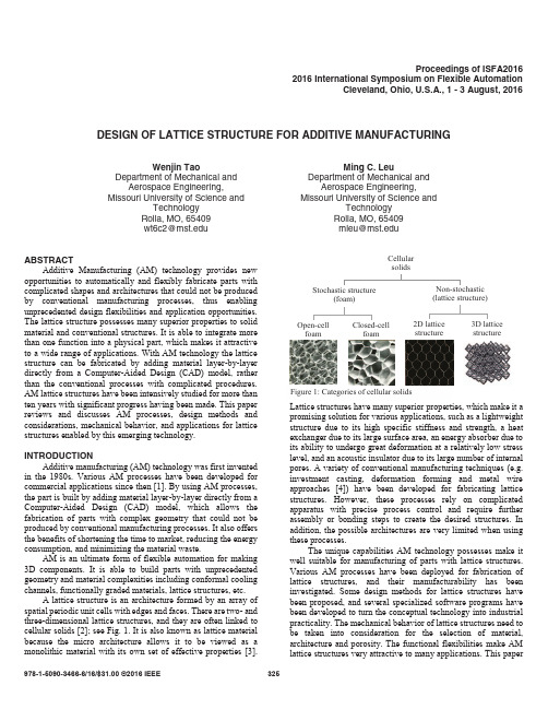
ABSTRACT Additive Manufacturing (AM) technology provides new opportunities to automatically and flexibly fabricate parts with complicated shapes and architectures that could not be produced by conventional manufacturing processes, thus enabling unprecedented design flexibilities and application opportunities. The lattice structure possesses many superior properties to solid material and conventional structures. It is able to integrate more than one function into a physical part, which makes it attractive to a wide range of applications. With AM technology the lattice structure can be fabricated by adding material layer-by-layer directly from a Computer-Aided Design (CAD) model, rather than the conventional processes with complicated procedures. AM lattice structures have been intensively studied for more than ten years with significant progress having been made. This paper reviews and discusses AM processes, design methods and considerations, mechanical behavior, and applications for lattice structures enabled by this emerging technology. INTRODUCTION Additive manufacturing (AM) technology was first invented in the 1980s. Various AM processes have been developed for commercial applications since then [1]. By using AM processes, the part is built by adding material layer-by-layer directly from a Computer-Aided Design (CAD) model, which allows the fabrication of parts with complex geometry that could not be produced by conventional manufacturing processes. It also offers the benefits of shortening the time to market, reducing the energy consumption, and minimizing the material waste. AM is an ultimate form of flexible automation for making 3D components. It is able to build parts with unprecedented geometry and material complexities including conformal cooling channels, functionally graded materials, lattice structures, etc. A lattice structure is an architecture formed by an array of spatial periodic unit cells with edges and faces. There are two- and three-dimensional lattice structures, and they are often linked to cellular solids [2]; see Fig. 1. It is also known as lattice material because the micro architecture allows it to be viewed as a monolithic material with its own set of effective properties [3].
apollo lattice算法边界约束

apollo lattice算法边界约束Apollo Lattice算法边界约束引言:Apollo Lattice(阿波罗格子)是一种用于解决大规模数据分析问题的算法。
该算法通过将数据划分成多个小规模的子数据集,并在每个子集上执行分析操作,从而实现高效的数据处理。
本文将重点讨论Apollo Lattice算法的边界约束,以及如何应用这些约束来优化数据分析过程。
一、Apollo Lattice算法简介Apollo Lattice算法是一种基于格子的数据分析算法。
它将数据集划分成多个格子,并在每个格子上执行分析操作。
这种划分的方式可以大大提高数据处理的效率,特别适用于大规模数据集的分析。
Apollo Lattice算法的核心思想是将数据集划分成多个小规模的子数据集,每个子数据集包含的数据量较少,从而可以在较短的时间内完成分析操作。
二、边界约束的作用边界约束是Apollo Lattice算法中的一个重要概念,它用于限制数据分析的边界范围。
边界约束可以帮助我们在数据处理过程中排除不必要的数据,从而提高数据分析的效率。
通过合理设置边界约束,可以减少数据的传输和处理量,降低算法的时间复杂度,从而加速数据分析的速度。
三、边界约束的应用场景边界约束可以应用于各种数据分析场景。
下面将介绍几个常见的应用场景。
1. 时间范围约束在某些数据分析场景中,我们可能只关心特定时间范围内的数据。
例如,在分析股票市场行情时,我们可能只关注最近一个月的数据。
通过设置时间范围的边界约束,我们可以只选择需要的数据,从而减少不必要的数据传输和处理。
2. 空间范围约束在某些地理信息系统(GIS)分析中,我们可能只关心特定地理区域内的数据。
通过设置空间范围的边界约束,我们可以排除不在该区域内的数据,从而减少数据传输和处理的工作量。
3. 数值范围约束在某些数据分析场景中,我们可能只关心特定数值范围内的数据。
例如,在分析销售数据时,我们可能只关注销售额在一定范围内的产品。
Petrel中文操作手册2010-(4~5章)
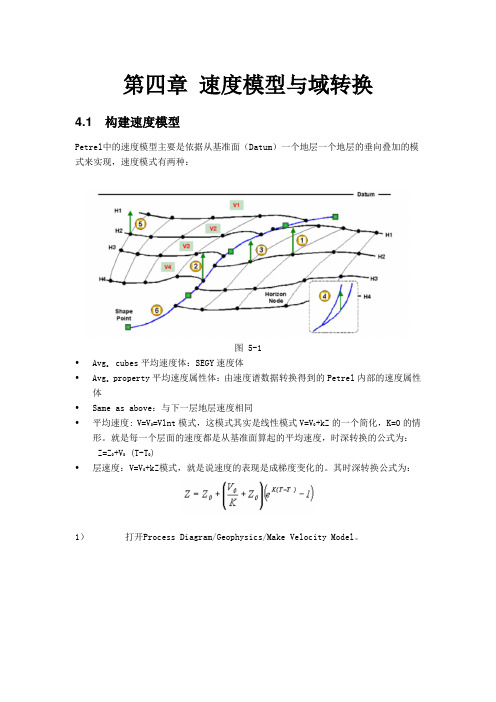
第四章速度模型与域转换4.1 构建速度模型Petrel中的速度模型主要是依据从基准面(Datum)一个地层一个地层的垂向叠加的模式来实现,速度模式有两种:图 5-1•Avg. cubes平均速度体:SEGY速度体•Avg. property平均速度属性体:由速度谱数据转换得到的Petrel内部的速度属性体•Same as above:与下一层地层速度相同•平均速度: V=V0=Vlnt模式,这模式其实是线性模式V=V0+kZ的一个简化,K=0的情形。
就是每一个层面的速度都是从基准面算起的平均速度,时深转换的公式为:Z=Z0+V0 (T-T0)•层速度:V=V0+kZ模式,就是说速度的表现是成梯度变化的。
其时深转换公式为:1)打开Process Diagram/Geophysics/Make Velocity Model。
图 5-22)在Petrel Explorer/Models中可以看到新生成的/,这个结果就是作时深转换的基础。
3)生成Velocity Models时可以选择output输出Time曲线、时深曲线、新的分层点等,进行质量控制。
图 5-3注意:当我们可以收集到等T0图和构造图(等深度图)这两种对应图件时,或者工区内有大量的井上分层数据资料时,我们可以通过Make Velocity Model的具体设置简化速度模型的人为分析。
图5-4 时深层面互校计算速度。
图5-5 时间层面和井上分层数据互校计算速度。
4.2 时间-深度转换1)确保Model Tab里面新计算获得的速度模型为激活的速度模型(粗体显示)。
2)在Input Tab里找到需要作时间-深度转换的地震数据,右键单击选择进行转换。
该步骤也可通过处理流程中Geophysics下面的弹出一个面板:图 5-63)如果是打开面板操作则可以选择不同类型的多种数据批量完成数据从时间域到深度域的转换。
第五章框架模型开始正式的建模操作之前,我们有必要整体的了解一下Process Diagram流程每个步骤的具体意义,以及各个步骤之间的联系。
A Label Field Fusion Bayesian Model and Its Penalized Maximum Rand Estimator for Image Segmentation

1610IEEE TRANSACTIONS ON IMAGE PROCESSING, VOL. 19, NO. 6, JUNE 2010A Label Field Fusion Bayesian Model and Its Penalized Maximum Rand Estimator for Image SegmentationMax MignotteAbstract—This paper presents a novel segmentation approach based on a Markov random field (MRF) fusion model which aims at combining several segmentation results associated with simpler clustering models in order to achieve a more reliable and accurate segmentation result. The proposed fusion model is derived from the recently introduced probabilistic Rand measure for comparing one segmentation result to one or more manual segmentations of the same image. This non-parametric measure allows us to easily derive an appealing fusion model of label fields, easily expressed as a Gibbs distribution, or as a nonstationary MRF model defined on a complete graph. Concretely, this Gibbs energy model encodes the set of binary constraints, in terms of pairs of pixel labels, provided by each segmentation results to be fused. Combined with a prior distribution, this energy-based Gibbs model also allows for definition of an interesting penalized maximum probabilistic rand estimator with which the fusion of simple, quickly estimated, segmentation results appears as an interesting alternative to complex segmentation models existing in the literature. This fusion framework has been successfully applied on the Berkeley image database. The experiments reported in this paper demonstrate that the proposed method is efficient in terms of visual evaluation and quantitative performance measures and performs well compared to the best existing state-of-the-art segmentation methods recently proposed in the literature. Index Terms—Bayesian model, Berkeley image database, color textured image segmentation, energy-based model, label field fusion, Markovian (MRF) model, probabilistic Rand index.I. INTRODUCTIONIMAGE segmentation is a frequent preprocessing step which consists of achieving a compact region-based description of the image scene by decomposing it into spatially coherent regions with similar attributes. This low-level vision task is often the preliminary and also crucial step for many image understanding algorithms and computer vision applications. A number of methods have been proposed and studied in the last decades to solve the difficult problem of textured image segmentation. Among them, we can cite clustering algorithmsManuscript received February 20, 2009; revised February 06, 2010. First published March 11, 2010; current version published May 14, 2010. This work was supported by a NSERC individual research grant. The associate editor coordinating the review of this manuscript and approving it for publication was Prof. Peter C. Doerschuk. The author is with the Département d’Informatique et de Recherche Opérationnelle (DIRO), Université de Montréal, Faculté des Arts et des Sciences, Montréal H3C 3J7 QC, Canada (e-mail: mignotte@iro.umontreal.ca). Color versions of one or more of the figures in this paper are available online at . Digital Object Identifier 10.1109/TIP.2010.2044965[1], spatial-based segmentation methods which exploit the connectivity information between neighboring pixels and have led to Markov Random Field (MRF)-based statistical models [2], mean-shift-based techniques [3], [4], graph-based [5], [6], variational methods [7], [8], or by region-based split and merge procedures, sometimes directly expressed by a global energy function to be optimized [9]. Years of research in segmentation have demonstrated that significant improvements on the final segmentation results may be achieved either by using notably more sophisticated feature selection procedures, or more elaborate clustering techniques (sometimes involving a mixture of different or non-Gaussian distributions for the multidimensional texture features [10], [11]) or by taking into account prior distribution on the labels, region process, or the number of classes [9], [12], [13]. In all cases, these improvements lead to computationally expensive segmentation algorithms and, in the case of energy-based segmentation models, to costly optimization techniques. The segmentation approach, proposed in this paper, is conceptually different and explores another strategy initially introduced in [14]. Instead of considering an elaborate and better designed segmentation model of textured natural image, our technique explores the possible alternative of fusing (i.e., efficiently combining) several quickly estimated segmentation maps associated with simpler segmentation models for a final reliable and accurate segmentation result. These initial segmentations to be fused can be given either by different algorithms or by the same algorithm with different values of the internal parameters such as several -means clustering results with different values of , or by several -means results using different distance metrics, and applied on an input image possibly expressed in different color spaces or by other means. The fusion model, presented in this paper, is derived from the recently introduced probabilistic rand index (PRI) [15], [16] which measures the agreement of one segmentation result to multiple (manually generated) ground-truth segmentations. This measure efficiently takes into account the inherent variation existing across hand-labeled possible segmentations. We will show that this non-parametric measure allows us to derive an appealing fusion model of label fields, easily expressed as a Gibbs distribution, or as a nonstationary MRF model defined on a complete graph. Finally, this fusion model emerges as a classical optimization problem in which the Gibbs energy function related to this model has to be minimized. In other words, or analytically expressed in the regularization framework, each quickly estimated segmentation (to be fused) provides a set of constraints in terms of pairs of pixel labels (i.e., binary cliques) that should be equal or not. Finally, our fusion result is found1057-7149/$26.00 © 2010 IEEEMIGNOTTE: LABEL FIELD FUSION BAYESIAN MODEL AND ITS PENALIZED MAXIMUM RAND ESTIMATOR FOR IMAGE SEGMENTATION1611by searching for a segmentation map that minimizes an energy function encoding this precomputed set of binary constraints (thus optimizing the so-called PRI criterion). In our application, this final optimization task is performed by a robust multiresolution coarse-to-fine minimization strategy. This fusion of simple, quickly estimated segmentation results appears as an interesting alternative to complex, computationally demanding segmentation models existing in the literature. This new strategy of segmentation is validated in the Berkeley natural image database (also containing, for quantitative evaluations, ground truth segmentations obtained from human subjects). Conceptually, our fusion strategy is in the framework of the so-called decision fusion approaches recently proposed in clustering or imagery [17]–[21]. With these methods, a series of energy functions are first minimized before their outputs (i.e., their decisions) are merged. Following this strategy, Fred et al. [17] have explored the idea of evidence accumulation for combining the results of multiple clusterings. Reed et al. have proposed a Gibbs energy-based fusion model that differs from ours in the likelihood and prior energy design, as final merging procedure (for the fusion of large scale classified sonar image [21]). More precisely, Reed et al. employed a voting scheme-based likelihood regularized by an isotropic Markov random field priorly used to inpaint regions where the likelihood decision is not available. More generally, the concept of combining classifiers for the improvement of the performance of individual classifiers is known, in machine learning field, as a committee machine or mixture of experts [22], [23]. In this context, Dietterich [23] have provided an accessible and informal reasoning, from statistical, computational and representational viewpoints, of why ensembles can improve results. In this recent field of research, two major categories of committee machines are generally found in the literature. Our fusion decision approach is in the category of the committee machine model that utilizes an ensemble of classifiers with a static structure type. In this class of committee machines, the responses of several classifiers are combined by means of a mechanism that does not involve the input data (contrary to the dynamic structure type-based mixture of experts). In order to create an efficient ensemble of classifiers, three major categories of methods have been suggested whose goal is to promote diversity in order to increase efficiency of the final classification result. This can be done either by using different subsets of the input data, either by using a great diversity of the behavior between classifiers on the input data or finally by using the diversity of the behavior of the input data. Conceptually, our ensemble of classifiers is in this third category, since we intend to express the input data in different color spaces, thus encouraging diversity and different properties such as data decorrelation, decoupling effects, perceptually uniform metrics, compaction and invariance to various features, etc. In this framework, the combination itself can be performed according to several strategies or criteria (e.g., weighted majority vote, probability rules: sum, product, mean, median, classifier as combiner, etc.) but, none (to our knowledge) uses the PRI fusion (PRIF) criterion. Our segmentation strategy, based on the fusion of quickly estimated segmentation maps, is similar to the one proposed in [14] but the criterion which is now used in this new fusion model is different. In [14], the fusion strategy can be viewed as a two-stephierarchical segmentation procedure in which the first step remains identical and a set of initial input texton segmentation maps (in each color space) is estimated. Second, a final clustering, taking into account this mixture of textons (expressed in the set of different color space) is then used as a discriminant feature descriptor for a final -mean clustering whose output is the final fused segmentation map. Contrary to the fusion model presented in this paper, this second step (fusion of texton segmentation maps) is thus achieved in the intra-class inertia sense which is also the so-called squared-error criterion of the -mean algorithm. Let us add that a conceptually different label field fusion model has been also recently introduced in [24] with the goal of blending a spatial segmentation (region map) and a quickly estimated and to-be-refined application field (e.g., motion estimation/segmentation field, occlusion map, etc.). The goal of the fusion procedure explained in [24] is to locally fuse label fields involving labels of two different natures at different level of abstraction (i.e., pixel-wise and region-wise). More precisely, its goal is to iteratively modify the application field to make its regions fit the color regions of the spatial segmentation with the assumption that the color segmentation is more detailed than the regions of the application field. In this way, misclassified pixels in the application field (false positives and false negatives) are filtered out and blobby shapes are sharpened, resulting in a more accurate final application label field. The remainder of this paper is organized as follows. Section II describes the proposed Bayesian fusion model. Section III describes the optimization strategy used to minimize the Gibbs energy field related to this model and Section IV describes the segmentation model whose outputs will be fused by our model. Finally, Section V presents a set of experimental results and comparisons with existing segmentation techniques.II. PROPOSED FUSION MODEL A. Rand Index The Rand index [25] is a clustering quality metric that measures the agreement of the clustering result with a given ground truth. This non-parametric statistical measure was recently used in image segmentation [16] as a quantitative and perceptually interesting measure to compare automatic segmentation of an image to a ground truth segmentation (e.g., a manually hand-segmented image given by an expert) and/or to objectively evaluate the efficiency of several unsupervised segmentation methods. be the number of pixels assigned to the same region Let (i.e., matched pairs) in both the segmentation to be evaluated and the ground truth segmentation , and be the number of pairs of pixels assigned to different regions (i.e., misand . The Rand index is defined as matched pairs) in to the total number of pixel pairs, i.e., the ratio of for an image of size pixels. More formally [16], and designate the set of region labels respecif tively associated to the segmentation maps and at pixel location and where is an indicator function, the Rand index1612IEEE TRANSACTIONS ON IMAGE PROCESSING, VOL. 19, NO. 6, JUNE 2010is given by the following relation:given by the empirical proportion (3) where is the delta Kronecker function. In this way, the PRI measure is simply the mean of the Rand index computed between each [16]. As a consequence, the PRI pair measure will favor (i.e., give a high score to) a resulting acceptable segmentation map which is consistent with most of the segmentation results given by human experts. More precisely, the resulting segmentation could result in a compromise or a consensus, in terms of level of details and contour accuracy exhibited by each ground-truth segmentations. Fig. 8 gives a fusion map example, using a set of manually generated segmentations exhibiting a high variation, in terms of level of details. Let us add that this probabilistic metric is not degenerate; all the bad segmentations will give a low score without exception [16]. C. Generative Gibbs Distribution Model of Correct Segmentations (i.e., the pairwise empirical As indicated in [15], the set ) defines probabilities for each pixel pair computed over an appealing generative model of correct segmentation for the image, easily expressed as a Gibbs distribution. In this way, the Gibbs distribution, generative model of correct segmentation, which can also be considered as a likelihood of , in the PRI sense, may be expressed as(1) which simply computes the proportion (value ranging from 0 to 1) of pairs of pixels with compatible region label relationships between the two segmentations to be compared. A value of 1 indicates that the two segmentations are identical and a value of 0 indicates that the two segmentations do not agree on any pair of points (e.g., when all the pixels are gathered in a single region in one segmentation whereas the other segmentation assigns each pixel to an individual region). When the number of and are much smaller than the number of data labels in points , a computationally inexpensive estimator of the Rand index can be found in [16]. B. Probabilistic Rand Index (PRI) The PRI was recently introduced by Unnikrishnan [16] to take into accounttheinherentvariabilityofpossible interpretationsbetween human observers of an image, i.e., the multiple acceptable ground truth segmentations associated with each natural image. This variability between observers, recently highlighted by the Berkeley segmentation dataset [26] is due to the fact that each human chooses to segment an image at different levels of detail. This variability is also due image segmentation being an ill-posed problem, which exhibits multiple solutions for the different possible values of the number of classes not known a priori. Hence, in the absence of a unique ground-truth segmentation, the clustering quality measure has to quantify the agreement of an automatic segmentation (i.e., given by an algorithm) with the variation in a set of available manual segmentations representing, in fact, a very small sample of the set of all possible perceptually consistent interpretations of an image [15]. The authors [16] address this concern by soft nonuniform weighting of pixel pairs as a means of accounting for this variability in the ground truth set. More formally, let us consider a set of manually segmented (ground truth) images corresponding to an be the segmentation to be compared image of size . Let with the manually labeled set and designates the set of reat pixel gion labels associated with the segmentation maps location , the probabilistic RI is defined bywhere is the set of second order cliques or binary cliques of a Markov random field (MRF) model defined on a complete graph (each node or pixel is connected to all other pixels of is the temperature factor of the image) and this Boltzmann–Gibbs distribution which is twice less than the normalization factor of the Rand Index in (1) or (2) since there than pairs of pixels for which are twice more binary cliques . is the constant partition function. After simplification, this yields(2) where a good choice for the estimator of (the probability of the pixel and having the same label across ) is simply (4)MIGNOTTE: LABEL FIELD FUSION BAYESIAN MODEL AND ITS PENALIZED MAXIMUM RAND ESTIMATOR FOR IMAGE SEGMENTATION1613where is a constant partition function (with a factor which depends only on the data), namelywhere is the set of all possible (configurations for the) segof size pixels. Let us add mentations into regions that, since the number of classes (and thus the number of regions) of this final segmentation is not a priori known, there are possibly, between one and as much as regions that the number of pixels in this image (assigning each pixel to an individual can region is a possible configuration). In this setting, be viewed as the potential of spatially variant binary cliques (or pairwise interaction potentials) of an equivalent nonstationary MRF generative model of correct segmentations in the case is assumed to be a set of representative ground where truth segmentations. Besides, , the segmentation result (to be ), can be considered as a realization of this compared to generative model with PRand, a statistical measure proportional to its negative likelihood energy. In other words, an estimate of , in the maximum likelihood sense of this generative model, will give a resulting segmented map (i.e., a fusion result) with a to be fused. high fidelity to the set of segmentations D. Label Field Fusion Model for Image Segmentation Let us consider that we have at our disposal, a set of segmentations associated to an image of size to be fused (i.e., to efficiently combine) in order to obtain a final reliable and accurate segmentation result. The generative Gibbs distribution model of correct segmentations expressed in (4) gives us an interesting fusion model of segmentation maps, in the maximum PRI sense, or equivalently in the maximum likelihood (ML) sense for the underlying Gibbs model expressed in (4). In this framework, the set of is computed with the empirical proportion estimator [see (3)] on the data . Once has been estimated, the resulting ML fusion segmentation map is thus defined by maximizing the likelihood distributiontions for different possible values of the number of classes which is not a priori known. To render this problem well-posed with a unique solution, some constraints on the segmentation process are necessary, favoring over segmentation or, on the contrary, merging regions. From the probabilistic viewpoint, these regularization constraints can be expressed by a prior distribution of treated as a realization of the unknown segmentation a random field, for example, within a MRF framework [2], [27] or analytically, encoded via a local or global [13], [28] prior energy term added to the likelihood term. In this framework, we consider an energy function that sets a particular global constraint on the fusion process. This term restricts the number of regions (and indirectly, also penalizes small regions) in the resulting segmentation map. So we consider the energy function (6) where designates the number of regions (set of connected pixels belonging to the same class) in the segmented is the Heaviside (or unit step) function, and an image , internal parameter of our fusion model which physically represents the number of classes above which this prior constraint, limiting the number of regions, is taken into account. From the probabilistic viewpoint, this regularization constraint corresponds to a simple shifted (from ) exponential distribution decreasing with the number of regions displayed by the final segmentation. In this framework, a regularized solution corresponds to the maximum a posteriori (MAP) solution of our fusion model, i.e., that maximizes the posterior distribution the solution , and thus(7) with is the regularization parameter controlling the contribuexpressing fidelity to the set of segtion of the two terms; encoding our prior knowledge or mentations to be fused and beliefs concerning the types of acceptable final segmentations as estimates (segmentation with a number of limited regions). In this way, the resulting criteria used in this resulting fusion model can be viewed as a penalized maximum rand estimator. III. COARSE-TO-FINE OPTIMIZATION STRATEGY A. Multiresolution Minimization Strategy Our fusion procedure of several label fields emerges as an optimization problem of a complex non-convex cost function with several local extrema over the label parameter space. In order to find a particular configuration of , that efficiently minimizes this complex energy function, we can use a global optimization procedure such as a simulated annealing algorithm [27] whose advantages are twofold. First, it has the capability of avoiding local minima, and second, it does not require a good solution. initial guess in order to estimate the(5) where is the likelihood energy term of our generative fusion . model which has to be minimized in order to find Concretely, encodes the set of constraints, in terms of pairs of pixel labels (identical or not), provided by each of the segmentations to be fused. The minimization of finds the resulting segmentation which also optimizes the PRI criterion. E. Bayesian Fusion Model for Image Segmentation As previously described in Section II-B, the image segmentation problem is an ill-posed problem exhibiting multiple solu-1614IEEE TRANSACTIONS ON IMAGE PROCESSING, VOL. 19, NO. 6, JUNE 2010Fig. 1. Duplication and “coarse-to-fine” minimization strategy.An alternative approach to this stochastic and computationally expensive procedure is the iterative conditional modes (ICM) introduced by Besag [2]. This method is deterministic and simple, but has the disadvantage of requiring a proper initialization of the segmentation map close to the optimal solution. Otherwise it will converge towards a bad local minima . In order associated with our complex energy function to solve this problem, we could take, as initialization (first such as iteration), the segmentation map (8) i.e., in choosing for the first iteration of the ICM procedure amongst the segmentation to be fused, the one closest to the optimal solution of the Gibbs energy function of our fusion model [see (5)]. A more robust optimization method consists of a multiresolution approach combined with the classical ICM optimization procedure. In this strategy, rather than considering the minimization problem on the full and original configuration space, the original inverse problem is decomposed in a sequence of approximated optimization problems of reduced complexity. This drastically reduces computational effort and provides an accelerated convergence toward improved estimate. Experimentally, estimation results are nearly comparable to those obtained by stochastic optimization procedures as noticed, for example, in [10] and [29]. To this end, a multiresolution pyramid of segmentation maps is preliminarily derived, in order to for each at different resolution levels, and a set estimate a set of of similar spatial models is considered for each resolution level of the pyramidal data structure. At the upper level of the pyramidal structure (lower resolution level), the ICM optimization procedure is initialized with the segmentation map given by the procedure defined in (8). It may also be initialized by a random solution and, starting from this initial segmentation, it iterates until convergence. After convergence, the result obtained at this resolution level is interpolated (see Fig. 1) and then used as initialization for the next finer level and so on, until the full resolution level. B. Optimization of the Full Energy Function Experiments have shown that the full energy function of our model, (with the region based-global regularization constraint) is complex for some images. Consequently it is preferable toFig. 2. From top to bottom and left to right; A natural image from the Berkeley database (no. 134052) and the formation of its region process (algorithm PRIF ) at the (l = 3) upper level of the pyramidal structure at iteration [0–6], 8 (the last iteration) of the ICM optimization algorithm. Duplication and result of the ICM relaxation scheme at the finest level of the pyramid at iteration 0, 1, 18 (last iteration) and segmentation result (region level) after the merging of regions and the taking into account of the prior. Bottom: evolution of the Gibbs energy for the different steps of the multiresolution scheme.perform the minimization in two steps. In a first step, the minimization is performed without considering the global constraint (considering only ), with the previously mentioned multiresolution minimization strategy and the ICM optimization procedure until its convergence at full resolution level. At this finest resolution level, the minimization is then refined in a second step by identifying each region of the resulting segmentation map. This creates a region adjacency graph (a RAG is an undirected graph where the nodes represent connected regions of the image domain) and performs a region merging procedure by simply applying the ICM relaxation scheme on each region (i.e., by merging the couple of adjacent regions leading to a reduction of the cost function of the full model [see (7)] until convergence). In the second step, minimization can also be performed . according to the full modelMIGNOTTE: LABEL FIELD FUSION BAYESIAN MODEL AND ITS PENALIZED MAXIMUM RAND ESTIMATOR FOR IMAGE SEGMENTATION1615with its four nearest neighbors and a fixed number of connections (85 in our application), regularly spaced between all other pixels located within a square search window of fixed size 30 pixels centered around . Fig. 3 shows comparison of segmentation results with a fully connected graph computed on a search window two times larger. We decided to initialize the lower (or third upper) level of the pyramid with a sequence of 20 different random segmentations with classes. The full resolution level is then initialized with the duplication (see Fig. 1) of the best segmentation result (i.e., the one associated to the lowest Gibbs energy ) obtained after convergence of the ICM at this lower resolution level (see Fig. 2). We provide details of our optimization strategy in Algorithm 1. Algo I. Multiresolution minimization procedure (see also Fig. 2). Two-Step Multiresolution Minimization Set of segmentations to be fusedPairwise probabilities for each pixel pair computed over at resolution level 1. Initialization Step • Build multiresolution Pyramids from • Compute the pairwise probabilities from at resolution level 3 • Compute the pairwise probabilities from at full resolution PIXEL LEVEL Initialization: Random initialization of the upper level of the pyramidal structure with classes • ICM optimization on • Duplication (cf. Fig 1) to the full resolution • ICM optimization on REGION LEVEL for each region at the finest level do • ICM optimization onFig. 4. Segmentation (image no. 385028 from Berkeley database). From top to bottom and left to right; segmentation map respectively obtained by 1] our multiresolution optimization procedure: = 3402965 (algo), 2] SA : = 3206127, 3] rithm PRIF : = 3312794, 4] SA : = 3395572, 5] SA : = 3402162. SAFig. 3. Comparison of two segmentation results of our multiresolution fusion procedure (algorithm PRIF ) using respectively: left] a subsampled and fixed number of connections (85) regularly spaced and located within a square search window of size = 30 pixels. right] a fully connected graph computed on a search window two times larger (and requiring a computational load increased by 100).NUU 0 U 00 U 0 U 0D. Comparison With a Monoresolution Stochastic Relaxation In order to test the efficiency of our two-step multiresolution relaxation (MR) strategy, we have compared it to a standard monoresolution stochastic relaxation algorithm, i.e., a so-called simulated annealing (SA) algorithm based on the Gibbs sampler [27]. In order to restrict the number of iterations to be finite, we have implemented a geometric temperature cooling schedule , where is the [30] of the form starting temperature, is the final temperature, and is the maximal number of iterations. In this stochastic procedure, is crucial. The temperathe choice of the initial temperature ture must be sufficiently high in the first stages of simulatedC. Algorithm In order to decrease the computational load of our multiresolution fusion procedure, we only use two levels of resolution in our pyramidal structure (see Fig. 2): the full resolution and an image eight times smaller (i.e., at the third upper level of classical data pyramidal structure). We do not consider a complete graph: we consider that each node (or pixel) is connected。
IDL中的IMSL
IDL Advanced及其详细功能介绍(2011-03-27 18:23:43)转载▼标签:分类:IDL数值分析idladvancedanalyst杂谈IDL Advanced是IDL的一个新的增值模块,它全面集成了IMSL TM C Numerical Library 的数学和统计程序,在IDL原有的交互式数据分析和可视化功能基础上增加了复杂的数学和统计功能。
IMSL(International Mathematics and Statistics Library)是由Visual Numerics,Inc 从20世纪70年代开始开发的包含全面的数学和统计函数的软件包,拥有超过300个已证明且精准的数学统计算法,IDL Advanced中包含了除金融方面函数之外的整个C语言库。
IDL Advanced为科学家和专业领域的工程师提供了185个经过证明的运算函数,在IDL 环境下,用户只需要简单地调用这些函数到自己的应用程序中,就可以实现复杂的数学和统计运算,并可以进行运算结果的快速可视化。
1. IMSL数学和统计功能列表:Linear System (线性系统)Eigensystem Analysis (特征系统分析)Interpolation and Approximation (差值和拟合)Quadrature (积分)Differential Equations (微分方程)Transforms (变换)Nonlinear Equations (非线性方程)Optimization (最优化)Special Functions (特殊函数)Basic Statistics and Random Number Generators (基础统计和随机数产生)Regression (回归)Correlation and Covariance (相关和协方差)Analysis of Variance (变异分析)Categorical and Discrete Data Analysis (分类和离散数据分析)Nonparametric Statistics (非参数统计)Goodness of Fit (拟和优度/配合度)Time Series and Forecasting (时间序列和预测)Multivariate Analysis (多元分析)Survival Analysis (生存分析)Probability Distribution Functions and Inverses (概率分布函数和反转)Random Number Generation (随机数生成)Math and Statistics Utilities(应用数学统计)2. IDL Advanced数学功能详细介绍§1 Linear System (线性系统)Matrix Inversion 矩阵转置IMSL_INVLinear Equations with Full Matrices 全矩阵线性方程IMSL_SP_LUSOLIMSL_SP_LUFACIMSL_SP_CHSOLIMSL_SP_CHFACLinear Least Squares with Full Matrices 全矩阵线性最小二乘IMSL_QRSOLIMSL_QRFACIMSL_SVDCOMPIMSL_CHNNDSOLIMSL_CHNNDFACIMSL_LINLSQSparse Matrices 稀疏矩阵IMSL_SP_LUSOLIMSL_SP_LUFACIMSL_SP_BDSOLIMSL_SP_BDFACIMSL_SP_PDSOLIMSL_SP_PDFACIMSL_SP_BDPDSOLIMSL_SP_BDPDFACIMSL_SP_GMRESIMSL_SP_CGIMSL_SP_MVMUL§2 Eigensystem Analysis (特征系统分析)Linear Eigensystem Problems 线性特征系统问题IMSL_EIGGeneralized Eigensystem Problems 广义特征系统问题IMSL_EIGSYMGENIMSL_GENEIG§3 Interpolation and Approximation (差值和拟合)Cubic Spline Interpolation 三次样条插值IMSL_CSINTERPIMSL_CSSHAPEB-spline Interpolation B-样条插值IMSL_BSINTERPIMSL_BSKNOTSB-spline and Cubic Spline Evaluation and Integration B-样条、三次样条评价及综合 IMSL_SPVALUEIMSL_SPINTEGLeast-squares Approximation and Smoothing 最小二乘拟和及滤波IMSL_FCNLSQIMSL_BSLSQIMSL_CONLSQIMSL_CSSMOOTHIMSL_SMOOTHDATA1DScattered Data Interpolation 离散数据插值IMSL_SCAT2DINTERPIMSL_RADBFIMSL_RADBE§4 Quadrature (积分)Univariate and Bivariate Quadrature 一元积分和双重积分IMSL_INTFCNArbitrary Dimension Quadrature 任意维的积分IMSL_INTFCNHYPERIMSL_INTFCN_QMCGauss Quadrature 高斯积分IMSL_GQUADDifferentiation 区别IMSL_FCN_DERIV§5 Differential Equations (微分方程)IMSL_ODEIMSL_PDE_MOLIMSL_POISSON2D§6 Transforms (变换)IMSL_FFTCOMPIMSL_FFTINITIMSL_CONVOL1DIMSL_CORR1DIMSL_LAPLACE_INV§7 Nonlinear Equations (非线性方程)Zeros of a Polynomial 多项式的零点IMSL_ZEROPOLYZeros of a Function 函数的零点IMSL_ZEROFCNRoot of a System of Equations 方程组的根IMSL_ZEROSYS§8 Optimization (最优化)Unconstrained Minimization 无约束最小化IMSL_FMINIMSL_FMINVIMSL_NLINLSQLinearly Constrained Minimization 线性约束最小化IMSL_LINPROGIMSL_QUADPROGNonlinearly Constrained Minimization 非线性约束最小化 IMSL_MINCONGENIMSL_CONSTRAINED_NLP§9 Special Functions (特殊函数)Error Functions 误差函数IMSL_ERFIMSL_ERFCIMSL_BETAIMSL_LNBETAIMSL_BETAIGamma Functions γ函数IMSL_LNGAMMAIMSL_GAMMA_ADVIMSL_GAMMAIBessel Functions with Real Order and Complex Argument 一般和复杂的贝赛尔函数 IMSL_BESSIIMSL_BESSJIMSL_BESSKIMSL_BESSYIMSL_BESSI_EXPIMSL_BESSK_EXPElliptic Integrals 椭圆积分IMSL_ELKIMSL_ELEIMSL_ELRFIMSL_ELRDIMSL_ELRJIMSL_ELRCFresnel Integrals菲涅耳积分IMSL_FRESNEL_COSINEIMSL_FRESNEL_SINEAiry Functions Airy函数IMSL_AIRY_AIIMSL_AIRY_BIKelvin Functions开尔文函数IMSL_KELVIN_BER0IMSL_KELVIN_BEI0IMSL_KELVIN_KER0IMSL_KELVIN_KEI03. IDL Advanced统计功能详细介绍§1 Basic Statistics (基础统计)Simple Summary Statistics 简单统计概要IMSL_NORM1SAMPIMSL_NORM2SAMPTabulate, Sort, and Rank 列表、分类和排列IMSL_FREQTABLEIMSL_SORTDATAIMSL_RANKS§2 Regression (回归)Multiple Linear Regression 多线性回归IMSL_REGRESSORSIMSL_MULTIREGRESSIMSL_MULTIPREDICTVariable Selection 变量选择IMSL_ALLBESTIMSL_STEPWISEPolynomial and Nonlinear Regression 多项式和非线性回归IMSL_POLYREGRESSIMSL_POLYPREDICTIMSL_NONLINREGRESSMultivariate Linear Regression—Statistical Inference and Diagnostics 多元线性回归-统计推断和诊断IMSL_HYPOTH_PARTIALIMSL_HYPOTH_SCPHIMSL_HYPOTH_TESTPolynomial and Nonlinear Regression 多项式和非线性回归IMSL_NONLINOPTAlternatives to Least Squares Regression 可选最小二乘回归IMSL_LNORMREGRESS§3 Correlation and Covariance (相关和协方差)IMSL_COVARIANCESIMSL_PARTIAL_COVIMSL_POOLED_COVIMSL_ROBUST_COV§4 Analysis of Variance (变异分析)IMSL_ANOVA1IMSL_ANOVAFACTIMSL_ANOVANESTEDIMSL_ANOVABALANCED§5 Categorical and Discrete Data Analysis (分类和离散数据分析)Statistics in the Two-Way Contingency Table (双向列联表统计)IMSL_CONTINGENCYIMSL_EXACT_ENUMIMSL_EXACT_NETWORKGeneralized Categorical Models 广义类别模型IMSL_CAT_GLM§6 Nonparametric Statistics (非参数统计)One Sample Tests—Nonparametric Statistics 单样本检验-非参数统计IMSL_SIGNTESTIMSL_WILCOXONIMSL_NCTRENDSIMSL_CSTRENDSIMSL_TIE_STATSTwo or More Samples Tests—Nonparametric Statistics 双样本或多样本检验-非参数统计 IMSL_KW_TESTIMSL_FRIEDMANS_TESTIMSL_COCHRANQIMSL_KTRENDS§7 Goodness of Fit (拟和优度/配合度)General Goodness of Fit Tests 一般拟和优度检验IMSL_CHISQTESTIMSL_NORMALITYIMSL_KOLMOGOROV1IMSL_KOLMOGOROV2IMSL_MVAR_NORMALITYTests for Randomness 随机检验IMSL_RANDOMNESS_TEST§8 Time Series and Forecasting (时间序列和预测)IMSL_ARMA Models IMSL_ARMA 模型IMSL_ARMAIMSL_DIFFERENCEIMSL_BOXCOXTRANSIMSL_AUTOCORRELATIONIMSL_PARTIAL_ACIMSL_LACK_OF_FITIMSL_GARCHIMSL_KALMAN§9 Multivariate Analysis (多元分析)IMSL_K_MEANSIMSL_PRINC_COMPIMSL_FACTOR_ANALYSISIMSL_DISCR_ANALYSIS§10 Survival Analysis (生存分析)IMSL_SURVIVAL_GLM§11 Probability Distribution Functions and Inverses (概率分布函数和反转) IMSL_NORMALCDFIMSL_BINORMALCDFIMSL_CHISQCDFIMSL_FCDFIMSL_TCDFIMSL_GAMMACDFIMSL_BETACDFIMSL_BINOMIALCDFIMSL_BINOMIALPDFIMSL_HYPERGEOCDFIMSL_POISSONCDF§12 Random Number Generation (随机数生成)Random Numbers 随机数IMSL_RANDOMOPTIMSL_RANDOM_TABLEIMSL_RANDOMIMSL_RANDOM_NPPIMSL_RANDOM_ORDERIMSL_RAND_TABLE_2WAYIMSL_RAND_ORTH_MATIMSL_RANDOM_SAMPLEIMSL_RAND_FROM_DATAIMSL_CONT_TABLEIMSL_RAND_GET_CONTIMSL_DISCR_TABLEIMSL_RAND_GEN_DISCRStochastic Processes 随机过程IMSL_RANDOM_ARMALow-discrepancy Sequences 超均匀分布序列IMSL_FAURE_INITIMSL_FAURE_NEXT_PT§13 Math and Statistics Utilities(应用数学统计)Dates 日期IMSL_DAYSTODATEIMSL_DATETODAYSConstants and Data Sets 常量和数据集IMSL_CONSTANTIMSL_MACHINEIMSL_STATDATABinomial Coefficient 二项式系数IMSL_BINOMIALCOEFGeometry 几何排列IMSL_NORMMatrix Norm 矩阵范数IMSL_MATRIX_NORMMatrix Entry and Display 矩阵输入和显示PMRM4.需要知道的关于IDL Advanced的几点常识:I.关于license:IDL Advanced是独立注册的IDL模块,如果没有安装IDL Advanced license,那么包含IMSL函数的IDL应用程序将不能运行,也就是说每个终端用户都必须有一个IDL Advanced license。
FLUENT中文全教程751-986
使用这个公式,select Implicit as the VOF Scheme, and enable an Unsteady calculation in the Solver panel (opened with the Define/Models/Solver... menu item).!!上面为the Euler explicit time-dependent formulation讨论的结果也适用于the implicit time-dependent formulation。
为了提高相界面的清晰度,你应慎重考虑以上所述。
5.Steady-state with the implicit interpolation scheme:如果你要寻找稳态解和中间的瞬态行为不感兴趣,并且最终的稳态解不被初始流动条件影响而每相有明显的inflow boundary,这个公式可以使用。
使用这个公式,select Implicit as the VOF Scheme.!!上面为Euler explicit time-dependent formulation讨论的结果也适用于the implicit steady-state formulation。
为了提高相界面的清晰度,你应慎重考虑以上所述。
!!对于the geometric reconstruction 和 donor-acceptor schemes,如果你使用了conformal grid(也就是,在两个子边界相交的边界上网格节点的位置是一样(identical)的),你必须保证在这个区域内没有双边(0厚度)壁面。
如果有,你必须split them, as described in Section 5.7.8.例子为了帮助为你的问题选择最好的公式,使用不同公式的例子列举如下:1.jet breakup:time-dependent with the geometric reconstruction scheme(or the donor-acceptor or Euler explicit scheme if problems occur with the geometric reconstruction scheme)。
CFD modeling to study fluidized bed combustion and gasication
* Corresponding author. Johan Gadolin Fellow, Process Chemistry Center, Abo Academy University, Abo, Finland. Tel.: þ91 (0)161 2560327; fax: þ91 161 2502240. E-mail address: dr.rjassar@ (R.I. Singh). 1 On EOL (without pay leave) from Department of Mechanical Engineering, Guru Nanak Dev Engineering College, Ludhiana, India. 1359-4311/$ e see front matter Ó 2012 Elsevier Ltd. All rights reserved. /10.1016/j.applthermaleng.2012.12.017
h i g h l i g h t s
< Summary of CFD modeling to study combustion/gasification in fluidized bed is done. < Equations for CFD modeling for fluidized bed combustion/gasification explained. < CFD modeling can predict heat flux, flow, temperature, ash deposits and emissions. < Trends, challenges and future research areas in this field are explored.
diffusion model介绍 -回复
diffusion model介绍-回复diffusion model是一种在认知心理学中广泛应用的模型,用于解释和预测人类决策和认知过程。
该模型基于信息传播的概念,通过模拟信息在人群中的传播和趋势形成,分析个体的选择和行为。
在解释diffusion model之前,首先需要了解一些其中涉及的基本概念,包括认知、决策和信息传播。
认知是指我们对于外界事物的感知、思考和理解过程,它涉及记忆、学习、注意力、知觉等方面的活动。
决策则是我们基于对信息的处理和评估,做出选择和行动的过程。
信息传播是指在社会、群体中信息的传递和扩散过程,它是人与人之间交流和互动的基础。
在diffusion model中,信息传播的过程被看作一个模型的基本元素。
这个信息可以是关于产品、服务、观念、观点等内容,可以通过传媒、口口相传、社交网络等途径传播。
diffusion model通过模拟信息的传播过程,来分析和预测人群对信息的接受和行为的变化。
diffusion model中的一个重要概念是创新。
创新是指新的产品、服务、观念等在市场中的第一次引入。
例如,一种新的智能手机,一项新的健康理念等。
创新可以通过不同的方式被人们接触到,比如广告、新闻报道等。
当人们接触到这个创新时,他们会基于自己对创新的认知和目标,做出选择和决策。
diffusion model中的另一个重要概念是创新的扩散。
创新的扩散是指当一些人接触到创新后,他们会通过交流和传播,使得更多的人了解和接受这个创新。
例如,当一些人购买了一种新款手机后,他们就会在社交媒体上分享使用心得,这样更多的人就会了解到这款手机并可能被其吸引。
这个过程可以将整个市场分为不同的群体,包括创新者、早期采纳者、早期多数和迟来者等。
每个群体的特点和行为方式都有所不同。
diffusion model在研究中涉及到一些参数和变量。
其中最核心的参数是创新的采纳率和创新的传播速度。
创新的采纳率表示在特定的时间段内,有多少人接受了这个创新。
- 1、下载文档前请自行甄别文档内容的完整性,平台不提供额外的编辑、内容补充、找答案等附加服务。
- 2、"仅部分预览"的文档,不可在线预览部分如存在完整性等问题,可反馈申请退款(可完整预览的文档不适用该条件!)。
- 3、如文档侵犯您的权益,请联系客服反馈,我们会尽快为您处理(人工客服工作时间:9:00-18:30)。
Yu-kui Zhou1 , 2
Mathematics Department, The Australian National University, Canberra, ACT 0200, Australia
Paul A. Pearce3
Abstract The fusion procedure is implemented for the dilute AL lattice models and a fusion hierarchy of functional equations with an su(3) structure is derived for the fused transfer matrices. We also present the Bethe ansatz equations for the dilute AL lattice models and discuss their connection with the fusion hierarchy. The solution of the fusion hierarchy for the eigenvalue spectra of the dilute AL lattice models will be presented in a subsequent paper.
arXiv:hep-th/9506108v1 17 Jun 1995
Mathematics Department, University of Melbourne, Parkville, Victoria 3052, Australia
ቤተ መጻሕፍቲ ባይዱ
Uwe Grimm4
Instituut voor Theoretische Fysica, Universiteit van Amsterdam, Valckenierstraat 65, 1018 XE Amsterdam, The Netherlands
2 1
1
however, are quite distinct and recent studies have shown that the dilute A–D –E models exhibit some new and very interesting aspects. First and foremost, in contrast to the AL model of Andrews, Baxter and Forrester [5], the dilute AL models, with L odd, can be solved [6] off-criticality in the presence of a symmetry-breaking field. In particular, in an appropriate regime, the dilute A3 model lies in the universality class of the Ising model in a magnetic field and gives the magnetic exponent δ = 15 [6]. In addition, Zamolodchikov [7] has argued that the magnetic Ising model in the scaling region is described by an E8 scattering theory. Accordingly, related E8 structures have recently been uncovered [8, 9] in the dilute A3 model. Lastly, the dilute A–D –E lattice models give [10] lattice realizations of the complete unitary minimal series of conformal field theories [11]. This again is not the case for the A–D –E models of Pasquier. An important step in the study of the AL models of Andrews, Baxter and Forrester (ABF) was the fusion [12] of the elementary weights to form new solutions of the YangBaxter equations. Subsequently, it was shown [13] that the transfer matrices of the fused ABF models satisfy special functional relations which can be solved for the eigenvalue spectra of these models. Moreover, at criticality, these equations can be solved for the central charges [13] and conformal weights [14]. Following the developments for the AL models of Andrews, Baxter and Forrester, we carry out in this paper the fusion procedure for the dilute AL lattice models and derive a fusion hierarchy of functional relations satisfied by the fused transfer matrices. The solution of this fusion hierarchy for the eigenvalue spectra, central charges and conformal weights will be given in a subsequent paper [15]. Historically, the fusion procedure was first introduced in [16]. It has since been successfully applied [17, 12, 18, 19, 20, 26] to many solvable models in two-dimensional statistical mechanics. The layout of this paper is as follows. In section 1.1 we define the dilute lattice models. In section 1.2 we present the Bethe ansatz for the commuting transfer matrices. Then in section 1.3 we discuss the fusion hierarchy and its connection to the Bethe ansatz. In section 2 we construct the fused face weights for elementary fusion. In section 3 we give in detail the procedure for constructing the completely symmetrically, (n, 0) and antisymmetrically (0, n) fused face weights. This is generalized in section 4 to construct the fused face weights for arbitrary fusion of mixed type (n, m). Finally, in section 5, we present the fusion hierarchy of functional relations and Bethe ansatz for the general fusion of mixed type (n, m). We summarize our results in section 6. 2
1.1
Dilute AL Lattice Models
The dilute AL lattice models [1] are restricted solid–on–solid (RSOS) models with L heights built on the AL Dynkin diagram as shown in Fig 1(a). The elements Aa,b of the adjacency matrix for this diagram are given by Aa,b = Ab,a =
hepth/9506108
1
Introduction
The dilute A–D –E lattice models [1, 2] are exactly solvable [3] restricted solid-on-solid (RSOS) models on the square lattice. These models resemble the A–D –E lattice models of Pasquier [4] in that the spins or heights take their values on a Dynkin diagram of a classical A–D –E Lie algebra. The properties of these two families of A–D –E models,