计量经济学导论第四版部分课后答案中文翻译
李子奈《计量经济学》(第4版)笔记和课后习题(含考研真题)详解
李子奈《计量经济学》(第4版)笔记和课后习题(含考研真题)详解李子奈《计量经济学》(第4版)笔记和课后习题详解第1章绪论一、计量经济学1计量经济学计量经济学,又称经济计量学,是由经济理论、统计学和数学结合而成的一门经济学的分支学科,其研究内容是分析经济现象中客观存在的数量关系。
2计量经济学模型(1)模型分类模型是对现实生活现象的描述和模拟。
根据描述和模拟办法的不同,对模型进行分类,如表1-1所示。
表1-1 模型分类(2)数理经济模型和计量经济学模型的区别①研究内容不同数理经济模型的研究内容是经济现象各因素之间的理论关系,计量经济学模型的研究内容是经济现象各因素之间的定量关系。
②描述和模拟办法不同数理经济模型的描述和模拟办法主要是确定性的数学形式,计量经济学模型的描述和模拟办法主要是随机性的数学形式。
③位置和作用不同数理经济模型可用于对研究对象的初步研究,计量经济学模型可用于对研究对象的深入研究。
3计量经济学的内容体系(1)根据所应用的数理统计方法划分广义计量经济学根据所应用的数理统计方法包括回归分析方法、投入产出分析方法、时间序列分析方法等;狭义计量经济学所应用的数理统计方法主要是回归分析方法。
需要注意的是,通常所述的计量经济学指的是狭义计量经济学。
(2)根据内容深度划分初级计量经济学的主要研究内容是计量经济学的数理统计学基础知识和经典的线性单方程计量经济学模型理论与方法;中级计量经济学的主要研究内容是用矩阵描述的经典的线性单方程计量经济学模型理论与方法、经典的线性联立方程计量经济学模型理论与方法,以及传统的应用模型;高级计量经济学的主要研究内容是非经典的、现代的计量经济学模型理论、方法与应用。
(3)根据研究目标和研究重点划分理论计量经济学的主要研究目标是计量经济学的理论与方法的介绍与研究;应用计量经济学的主要研究目标是计量经济学模型的建立与应用。
理论计量经济学的研究重点是理论与方法的数学证明与推导;应用计量经济学的研究重点是建立和应用计量模型处理实际问题。
计量经济学导论(四版)十三章习题答案(中文版)

计量经济学导论(四版)十三章习题答案(中文版)计量经济学导论十三章习题答案(中文版)13.1在其他解释变量的平均值不变的情况下,1972到1984年的平均生育率下降0.545,这就是y84的系数值。
考虑到教育平均数瓶的增加,我们将增加额外的效应:–.128(13.3 –12.2) ≈–.141.所以总共的效应为:.545 + .141 =.68613.3因为在每个时期的独立横截面数据中都没有重复的观测值,因此对一对数据进行差分是没有意义的。
例如在例子13,1中,同一个妇女出现在多余一年数据中是不太可能的,因为每一年中得到的都是新的随机样本。
在例子13.3中,一些房屋可能同时出现在1981和1978奶奶,但是重叠的可能性太小以至于不能做一个真正的面板数据分析。
13.5我们不嗯呢该在元模型中包含年龄作为解释变量。
面板数据中的每一个人实际上在1992年1月31日都比1990年1月31日大两岁。
这就意味着Δagei= 2 对所有的i.。
但是我们要估计的方程形式是:Δsavingi= δ0 + β1Δagei+ …,这里δ0在元模型中是1992年虚拟变量的系数。
我们知道,当模型中含有截距的时候我们就不能再加入一个对i来说是常数的解释变量;这违反了假设MLR.3.直觉上的,既然年龄的变化对每个人都是相同的没我们就不能从加总的时间上区分年龄的效应。
13.7(1)这并不令我们吃惊,因为afchnge在(3.12) 中的系数仅为.0077(t统计量也很小)。
系数从.191 到.198的增加轻易地解释了样本误差。
(2)如果从方程中去掉highearn,那么我们就是假设,在政策变动之前,在高收入和低收入人群中的平均离岗周数没有区别。
但是世界上是非常大的(.256),而且在3.12中highearn估计是统计上显著的表明这种前提假设是错误的。
在政策变动前,高收入群体大约比低收入群体在失业补偿金中多花费约29.2% [ exp(.256) ?1≈.292 ]。
计量经济学导论第四版部分课后答案中文翻译
2.10(iii) From (2.57), Var(1ˆβ) = σ2/21()n i i x x =⎛⎫- ⎪⎝⎭∑. 由提示:: 21n i i x=∑ ≥21()n i i x x =-∑, and so Var(1β ) ≤ Var(1ˆβ). A more direct way to see this is to write(一个更直接的方式看到这是编写) 21()n ii x x =-∑ = 221()n i i x n x =-∑, which is less than21n i i x=∑unless x = 0.(iv)给定的c 2i x 但随着x 的增加, 1ˆβ的方差与Var(1β )的相关性也增加.0β小时1β 的偏差也小.因此, 在均方误差的基础上不管我们选择0β还是1β 要取决于0β,x ,和n 的大小 (除了 21n i i x=∑的大小).3.7We can use Table 3.2. By definition, 2β > 0, and by assumption, Corr(x 1,x 2) < 0. Therefore, there is anegative bias in 1β : E(1β ) < 1β. This means that, on average across different random samples, the simple regression estimator underestimates the effect of the training program. It is even possible that E(1β ) is negative even though 1β > 0. 我们可以使用表3.2。
根据定义,> 0,由假设,科尔(X1,X2)<0。
因此,有一个负偏压为:E ()<。
计量经济学(第四版)习题及参考答案解析详细版

计量经济学(第四版)习题参考答案潘省初第一章 绪论1.1 试列出计量经济分析的主要步骤。
一般说来,计量经济分析按照以下步骤进行:(1)陈述理论(或假说) (2)建立计量经济模型 (3)收集数据 (4)估计参数 (5)假设检验 (6)预测和政策分析 1.2 计量经济模型中为何要包括扰动项?为了使模型更现实,我们有必要在模型中引进扰动项u 来代表所有影响因变量的其它因素,这些因素包括相对而言不重要因而未被引入模型的变量,以及纯粹的随机因素。
1.3什么是时间序列和横截面数据? 试举例说明二者的区别。
时间序列数据是按时间周期(即按固定的时间间隔)收集的数据,如年度或季度的国民生产总值、就业、货币供给、财政赤字或某人一生中每年的收入都是时间序列的例子。
横截面数据是在同一时点收集的不同个体(如个人、公司、国家等)的数据。
如人口普查数据、世界各国2000年国民生产总值、全班学生计量经济学成绩等都是横截面数据的例子。
1.4估计量和估计值有何区别?估计量是指一个公式或方法,它告诉人们怎样用手中样本所提供的信息去估计总体参数。
在一项应用中,依据估计量算出的一个具体的数值,称为估计值。
如Y就是一个估计量,1nii YY n==∑。
现有一样本,共4个数,100,104,96,130,则根据这个样本的数据运用均值估计量得出的均值估计值为5.107413096104100=+++。
第二章 计量经济分析的统计学基础2.1 略,参考教材。
2.2请用例2.2中的数据求北京男生平均身高的99%置信区间NS S x ==45=1.25 用α=0.05,N-1=15个自由度查表得005.0t =2.947,故99%置信限为 x S t X 005.0± =174±2.947×1.25=174±3.684也就是说,根据样本,我们有99%的把握说,北京男高中生的平均身高在170.316至177.684厘米之间。
计量经济学(第四版)习题参考答案
第一章 绪论1.1 一般说来,计量经济分析按照以下步骤进行:(1)陈述理论(或假说) (2)建立计量经济模型 (3)收集数据(4)估计参数 (5)假设检验 (6)预测和政策分析 1.2 我们在计量经济模型中列出了影响因变量的解释变量,但它(它们)仅是影响因变量的主要因素,还有很多对因变量有影响的因素,它们相对而言不那么重要,因而未被包括在模型中。
为了使模型更现实,我们有必要在模型中引进扰动项u 来代表所有影响因变量的其它因素,这些因素包括相对而言不重要因而未被引入模型的变量,以及纯粹的随机因素。
1.3时间序列数据是按时间周期(即按固定的时间间隔)收集的数据,如年度或季度的国民生产总值、就业、货币供给、财政赤字或某人一生中每年的收入都是时间序列的例子。
横截面数据是在同一时点收集的不同个体(如个人、公司、国家等)的数据。
如人口普查数据、世界各国2000年国民生产总值、全班学生计量经济学成绩等都是横截面数据的例子。
1.4 估计量是指一个公式或方法,它告诉人们怎样用手中样本所提供的信息去估计总体参数。
在一项应用中,依据估计量算出的一个具体的数值,称为估计值。
如Y 就是一个估计量,1nii YY n==∑。
现有一样本,共4个数,100,104,96,130,则根据这个样本的数据运用均值估计量得出的均值估计值为5.107413096104100=+++。
第二章 计量经济分析的统计学基础2.1 略,参考教材。
2.2N SS x ==45=1.25 用α=0.05,N-1=15个自由度查表得005.0t =2.947,故99%置信限为x S t X 005.0± =174±2.947×1.25=174±3.684也就是说,根据样本,我们有99%的把握说,北京男高中生的平均身高在170.316至177.684厘米之间。
2.3 原假设120:0=μH备择假设120:1≠μH检验统计量()10/25XX μσ-Z ====查表96.1025.0=Z 因为Z= 5 >96.1025.0=Z ,故拒绝原假设, 即此样本不是取自一个均值为120元、标准差为10元的正态总体。
伍德里奇《计量经济学导论》(第4版)笔记和课后习题详解-第1~4章【圣才出品】

Байду номын сангаас
2.假设让你进行一项研究,以确定较小的班级规模是否会提高四年级学生的成绩。
4 / 119
圣才电子书 十万种考研考证电子书、题库视频学习平台
(i)如果你能设定你想做的任何实验,你想做些什么?请具体说明。 (ii)更现实地,假设你能搜集到某个州几千名四年级学生的观测数据。你能得到他们 四年级班级规模和四年级末的标准化考试分数。你为什么预计班级规模与考试成绩存在负相 关关系? (iii)负相关关系一定意味着较小的班级规模会导致更好的成绩吗?请解释。 答:(i)假定能够随机的分配学生们去不同规模的班级,也就是说,在不考虑学生诸如 能力和家庭背景等特征的前提下,每个学生被随机的分配到不同的班级。因此可以看到班级 规模(在伦理考量和资源约束条件下的主体)的显著差异。 (ii)负相关关系意味着更大的班级规模与更差的考试成绩是有直接联系的,因此可以 发现班级规模越大,导致考试成绩越差。 通过数据可知,两者之间的负相关关系还有其他的原因。例如,富裕家庭的孩子在学校 可能更多的加入小班,而且他们的成绩优于平均水平。 另外一个可能性是:学校的原则是将成绩较好的学生分配到小班。或者部分父母可能坚 持让自己的孩子进入更小的班级,而同样这些父母也更多的参与子女的教育。 (iii)鉴于潜在的其他混杂因素(如 ii 所列举),负相关关系并不一定意味着较小的班 级规模会导致更好的成绩。控制混杂因素的方法是必要的,而这正是多重回归分析的主题。
伍德里奇计量经济学导论第四版

15CHAPTER 3TEACHING NOTESFor undergraduates, I do not work through most of the derivations in this chapter, at least not in detail. Rather, I focus on interpreting the assumptions, which mostly concern the population. Other than random sampling, the only assumption that involves more than populationconsiderations is the assumption about no perfect collinearity, where the possibility of perfect collinearity in the sample (even if it does not occur in the population should be touched on. The more important issue is perfect collinearity in the population, but this is fairly easy to dispense with via examples. These come from my experiences with the kinds of model specification issues that beginners have trouble with.The comparison of simple and multiple regression estimates – based on the particular sample at hand, as opposed to their statistical properties – usually makes a strong impression. Sometimes I do not bother with the “partialling out” interpretation of multiple regression.As far as statistical properties, notice how I treat the problem of including an irrelevant variable: no separate derivation is needed, as the result follows form Theorem 3.1.I do like to derive the omitted variable bias in the simple case. This is not much more difficult than showing unbiasedness of OLS in the simple regression case under the first four Gauss-Markov assumptions. It is important to get the students thinking aboutthis problem early on, and before too many additional (unnecessary assumptions have been introduced.I have intentionally kept the discussion of multicollinearity to a minimum. This partly indicates my bias, but it also reflects reality. It is, of course, very important for students to understand the potential consequences of having highly correlated independent variables. But this is often beyond our control, except that we can ask less of our multiple regression analysis. If two or more explanatory variables are highly correlated in the sample, we should not expect to precisely estimate their ceteris paribus effects in the population.I find extensive treatments of multicollinearity, where one “tests” or somehow “solves” the multicollinearity problem, to be misleading, at best. Even the organization of some texts gives the impression that imperfect multicollinearity is somehow a violation of the Gauss-Markovassumptions: they include multicollinearity in a chapter or part of the book devoted to “violation of the basic assumptions,” or something like that. I have noticed that master’s students who have had some undergraduate econometrics are often confused on the multicollinearity issue. It is very important that students not confuse multicollinearity among the included explanatory variables in a regression model with the bias caused by omitting an important variable.I do not prove the Gauss-Markov theorem. Instead, I emphasize its implications. Sometimes, and certainly for advanced beginners, I put a special case of Problem 3.12 on a midterm exam, where I make a particular choice for the function g (x . Rather than have the students directly 课后答案网ww w.kh d aw .c om16compare the variances, they should appeal to the Gauss-Markov theorem for the superiority of OLS over any other linear, unbiased estimator.SOLUTIONS TO PROBLEMS3.1 (i Yes. Because of budget constraints, it makes sense that, the more siblings there are in a family, the less education any one child in the family has. To find the increase in the number of siblings that reduces predicted education by one year, we solve 1 = .094(Δsibs , so Δsibs = 1/.094 ≈ 10.6.(ii Holding sibs and feduc fixed, one more year of mother’s education implies .131 years more of predicted education. So if a mother has four more years of education, her son is predicted to have about a half a year (.524 more years of education. (iii Since the number of siblings is the same, but meduc and feduc are both different, the coefficientson meduc and feduc both need to be accounted for. The predicted difference in education between B and A is .131(4 + .210(4 = 1.364.3.2 (i hsperc is defined so that the smaller it is, the lower the student’s standing in high school. Everything else equal, the worse the student’s standing in high school, the lower is his/her expected college GPA. (ii Just plug these values into the equation:n colgpa= 1.392 − .0135(20 + .00148(1050 = 2.676.(iii The difference between A and B is simply 140 times the coefficient on sat , because hsperc is the same for both students. So A is predicted to have ascore .00148(140 ≈ .207 higher.(iv With hsperc fixed, n colgpaΔ = .00148Δsat . Now, we want to find Δsat such that n colgpaΔ = .5, so .5 = .00148(Δsat or Δsat = .5/(.00148 ≈ 338. Perhaps not surprisingly, a large ceteris paribus difference in SAT score – almost two and one-half standard deviations – is needed to obtain a predicted difference in college GPA or a half a point.3.3 (i A larger rank for a law school means that the school has less prestige; this lowers starting salaries. For example, a rank of 100 means there are 99 schools thought to be better.课后答案网ww w.kh d aw .c om17(ii 1β > 0, 2β > 0. Both LSAT and GPA are measures of the quality of the entering class. No matter where better students attend law school, we expect them to earn more, on average. 3β, 4β > 0. The numbe r of volumes in the law library and the tuition cost are both measures of the school quality. (Cost is less obvious than library volumes, but should reflect quality of the faculty, physical plant, and so on. (iii This is just the coefficient on GPA , multiplied by 100: 24.8%. (iv This is an elasticity: a one percent increase in library volumes implies a .095% increase in predicted median starting salary, other things equal. (v It is definitely better to attend a law school with a lower rank. If law school A has a ranking 20 less than law school B, the predicted difference in starting salary is 100(.0033(20 = 6.6% higher for law school A.3.4 (i If adults trade off sleep for work, more work implies less sleep (other things equal, so 1β < 0. (ii The signs of 2β and 3β are not obvious, at least to me. One could argue that more educated people like to get more out of life, and so, other things equal,they sleep less (2β < 0. The relationship between sleeping and age is more complicated than this model suggests, and economists are not in the best position to judge such things.(iii Since totwrk is in minutes, we must convert five hours into minutes: Δtotwrk = 5(60 = 300. Then sleep is predicted to fall by .148(300 = 44.4 minutes. For a week, 45 minutes less sleep is not an overwhelming change. (iv More education implies less predicted time sleeping, but the effect is quite small. If we assume the difference between college and high school is four years, the college graduate sleeps about 45 minutes less per week, other things equal. (v Not surprisingly, the three explanatory variables explain only about 11.3% of the variation in sleep . One important factor in the error term is general health. Another is marital status, and whether the person has children. Health (however we measure that, marital status, and number and ages of children would generally be correlated with totwrk . (For example, less healthy people would tend to work less.3.5 Conditioning on the outcomes of the explanatory variables, we have 1E(θ =E(1ˆβ + 2ˆβ = E(1ˆβ+ E(2ˆβ = β1 + β2 = 1θ.3.6 (i No. By definition, study + sleep + work + leisure = 168. Therefore, if we change study , we must change at least one of the other categories so that the sum is still 168. 课后答案网ww w.kh d aw .c om18(ii From part (i, we can write, say, study as a perfect linear function of the otherindependent variables: study = 168 − sleep − work − leisure . This holds for every observation, so MLR.3 violated. (iii Simply drop one of the independent variables, say leisure :GPA = 0β + 1βstudy + 2βsleep + 3βwork + u .Now, for example, 1β is interpreted as the change in GPA when study increases by one hour, where sleep , work , and u are all held fixed. If we are holding sleep and work fixed but increasing study by one hour, then we must be reducing leisure by one hour. The other slope parameters have a similar interpretation.3.7 We can use Table 3.2. By definition, 2β > 0, and by assumption, Corr(x 1,x 2 < 0.Therefore, there is a negative bias in 1β: E(1β < 1β. This means that, on average across different random samples, the simple regression estimator underestimates the effect of thetraining program. It is even possible that E(1β is negative even though 1β > 0.3.8 Only (ii, omitting an important variable, can cause bias, and this is true only when the omitted variable is correlated with the included explanatory variables. The homoskedasticity assumption, MLR.5, played no role in showing that the OLS estimators are unbiased.(Homoskedasticity was used to o btain the usual variance formulas for the ˆjβ. Further, the degree of collinearity between the explanatory variables in the sample, even if it is reflected in a correlation as high as .95, does not affect the Gauss-Markov assumptions. Only if there is a perfect linear relationship among two or more explanatory variables is MLR.3 violated.3.9 (i Because 1x is highly correlated with 2x and 3x , and these latter variables have largepartial effects on y , the simple and multiple regression coefficients on 1x can differ by largeamounts. We have not done this case explicitly, but given equation (3.46 and the discussion with a single omitted variable, the intuition is pretty straightforward.(ii Here we would expect 1β and 1ˆβ to be similar (subject, of course, to what we mean by “almost uncorrelated”. The amount of correlation between 2x and 3x does not directly effect the multiple regression estimate on 1x if 1x is essentially uncorrelated with 2x and 3x .(iii In this case we are (unnecessarily introducing multicollinearity into the regression: 2x and 3x have small partial effects on y and yet 2x and 3x are highly correlated with 1x . Adding2x and 3x like increases the standard error of the coefficient on 1x substantially, so se(1ˆβis likely to be much larger than se(1β . 课后答案网ww w.kh d aw .c om19(iv In this case, adding 2x and 3x will decrease the residual variance without causingmuch collinearity (because 1x is almost uncorrelated with 2x and 3x , so we should see se(1ˆβ smaller than se(1β. The amount of correlation between 2x and 3x does not directly affect se(1ˆβ.3.10 From equation (3.22 we have111211ˆ,ˆni ii ni i r yr β===∑∑where the 1ˆi rare defined in the problem. As usual, we must plug in the true model for y i : 1011223311211ˆ(.ˆni i i i ii ni i r x x x u r βββββ==++++=∑∑The numerator of this expression simplifies because 11ˆni i r=∑ = 0, 121ˆni i i r x =∑ = 0, and 111ˆni i i r x =∑ = 211ˆni i r =∑. These all follow from the fact that the 1ˆi rare the residuals from the regression of 1i x on 2i x : the 1ˆi rhave zero sample average and are uncorrelated in sample with 2i x . So the numerator of 1βcan be expressed as2113131111ˆˆˆ.n n ni i i i i i i i rr x r u ββ===++∑∑∑Putting these back over the denominator gives 13111113221111ˆˆ.ˆˆnni i ii i nni i i i r x rur r βββ=====++∑∑∑∑课后答案网ww w.kh d aw .c om20Conditional on all sample values on x 1, x 2, and x 3, only the last term is random due to its dependence on u i . But E(u i = 0, and so131113211ˆE(=+,ˆni i i ni i r xr βββ==∑∑which is what we wanted to show. Notice that the term multiplying 3β is the regressioncoefficient from the simple regression of x i 3 on 1ˆi r.3.11 (i 1β < 0 because more pollution can be expected to lower housing values; note that 1β isthe elasticity of price with respect to nox . 2β is probably positive because rooms roughlymeasures the size of a house. (However, it does not allow us to distinguish homes where each room is large from homes where each room is small. (ii If we assume that rooms increases with quality of the home, then log(nox and rooms are negatively correlated when poorer neighborhoods have more pollution, something that is often true. We can use Ta ble 3.2 to determine the direction of the bias. If 2β > 0 andCorr(x 1,x 2 < 0, the simple regression estimator 1βhas a downward bias. But because 1β < 0, this means that the simple regression, on average, overstates the importance of pollution. [E(1β is more negative than 1β.] (iii This is what we expect from the typical sample based on our analysis in part (ii. The simple regression estimate, −1.043, is more negative (larger in magnitude than the multiple regression estimate, −.718. As those estimates are only for one sample, we can never know which is closer to 1β. But if this is a “typical” sample, 1β is closer to −.718.3.12 (i For notational simplicity, define s zx = 1(;ni i i z z x =−∑ this is not quite the samplecovariance between z and x because we do not divide by n – 1, but we are only using it tosimplify notation. Then we can write 1β as11(.niii zxz z ys β=−=∑This is clearly a linear function of the y i : take the weights to be w i = (z i −z /s zx . To show unbiasedness, as usual we plug y i = 0β + 1βx i + u i into this equation, and simplify: 课后答案网w w w .k h d aw .c o m21 11 1 011 111(( (((n ii i i zxnni zx i ii i zxniii zxz z x u s z z s z z u s zz u s ββββββ====−++=−++−=−=+∑∑∑∑where we use the fact that 1(ni i z z =−∑ = 0 always. Now s zx is a function of the z i and x i and theexpected value of each u i is zero conditional on all z i and x i in the sample. Therefore, conditional on these values,1111(E(E(niii zxz z u s βββ=−=+=∑because E(u i = 0 for all i . (ii From the fourth equation in part (i we have (again conditional on the z i and x i in the sample,2111222212Var ((Var(Var((n ni i i i i i zx zxnii zxz z u z z u s s z z s βσ===⎡⎤−−⎢⎥⎣⎦==−=∑∑∑because of the homoskedasticit y assumption [Var(u i = σ2 for all i ]. Given the definition of s zx , this is what we wanted to show.课后答案网ww w.kh d aw .c om22(iii We know that Var(1ˆβ = σ2/21[(].ni i x x =−∑ Now we can rearrange the inequality in the hint, drop x from the sample covariance, and cancel n -1everywhere, to get 221[(]/ni zx i z z s =−∑ ≥211/[(].ni i x x =−∑ When we multiply through by σ2 we get Var(1β ≥ Var(1ˆβ, which is what we wanted to show.3.13 (i The shares, by definition, add to one. If we do not omit one of the shares then the equation would suffer from perfect multicollinearity. The parameters would not have a ceteris paribus interpretation, as it is impossible to change one share while holding all of the other shares fixed. (ii Because each share is a proportion (and can be at most one, when all other shares are zero, it makes little sense to increase share p by one unit. If share p increases by .01 – which is equivalent to a one percentage point increase in the share of property taxes in total revenue – holding share I , share S , and the other factorsfixed, then growth increases by 1β(.01. With the other shares fixed, the excluded share, share F , must fall by .01 when share p increases by .01.SOLUTIONS TO COMPUTER EXERCISESC3.1 (i Prob ably 2β > 0, as more income typically means better nutrition for the mother and better prenatal care. (ii On the one hand, an increase in income generally increases the consumption of a good, and cigs and faminc could be positively correlated. On the other, family incomes are also higher for families with more education, and more education and cigarette smoking tend to benegatively correlated. The sample correlation between cigs and faminc is about −.173, indicating a negative correlation.(iii The regressions without and with faminc aren 119.77.514bwghtcigs =−21,388,.023n R ==and n 116.97.463.093bwghtcigs faminc =−+21,388,.030.n R ==课后答案网ww w.kh d aw .c om23The effect of cigarette smoking is slightly smaller when faminc is added to the regression, but the difference is not great. This is due to the fact that cigs and faminc are not very correlated, and the coefficient on faminc is practically small. (The variable faminc is measured in thousands, so $10,000 more in 1988 income increases predicted birth weight by only .93 ounces.C3.2 (i The estimated equation isn 19.32.12815.20price sqrft bdrms =−++288,.632n R ==(ii Holding square footage constant, n price Δ = 15.20 ,bdrms Δ and so n price increases by 15.20, which means $15,200.(iii Now n price Δ = .128sqrft Δ + 15.20bdrms Δ = .128(140 + 15.20 = 33.12, or $33,120. Because the size of the house is increasing, this is a much larger effect than in (ii. (iv About 63.2%. (v The predicted price is –19.32 + .128(2,438 + 15.20(4 = 353.544, or $353,544. (vi From part (v, the estimated value of the home based only on square footage and number of bedrooms is $353,544. The actual selling price was $300,000, which suggests the buyer underpaid by some margin. But, of course, there are many other features of a house (some that we cannot even measure that affect price, and we have not controlled for these.C3.3 (i The constant elasticity equation isn log( 4.62.162log(.107log(salary sales mktval =++ 2177,.299.n R ==(ii We cannot include profits in logarithmic form because profits are negative for nine of the companies in the sample. When we add it in levels form we getn log( 4.69.161log(.098log(.000036salary sales mktval profits =+++2177,.299.n R ==The coefficient on profits is very small. Here, profits are measured in millions, so if profits increase by $1 billion, which means profits Δ = 1,000 – a huge change – predicted salaryincreases by about only 3.6%. However, remember that we are holding sales and market value fixed.课后答案网ww w.kh d aw .c om24Together, these variables (and we could drop profits without losing anything explain almost 30% of the sample variation in log(salary . This is certainly not “most” of the variation.(iii Adding ceoten to the equation givesn log( 4.56.162log(.102log(.000029.012salary sales mktval profits ceoten =++++2177,.318.n R ==This means that one more year as CEO increases predicted salary by about 1.2%. (iv The sample correlation between log(mktval and profits is about .78, which is fairly high. As we know, this causes no bias in the OLS estimators, although it can cause their variances to be large. Given the fairly substantial correlation between market value andfirm profits, it is not too surprising that the latter adds nothing to explaining CEO salaries. Also, profits is a short term measure of how the firm is doing while mktval is based on past, current, and expected future profitability.C3.4 (i The minimum, maximum, and average values for these three variables are given in the table below:Variable Average Minimum Maximum atndrte priGPA ACT 81.71 2.59 22.516.25 .86131003.93 32(ii The estimated equation isn 75.7017.26 1.72atndrtepriGPA ACT =+− n = 680, R 2 = .291.The intercept means that, for a student whose prior GPA is zero and ACT score is zero, the predicted attendance rate is 75.7%. But this is clearly not an interesting segment of thepopulation. (In fact, there are no students in the college population with priGPA = 0 and ACT = 0, or with values even close to zero. (iii The coefficient on priGPA means that, if a student’s prior GPA is one point higher (say, from 2.0 to 3.0, the attendance rate is about 17.3 percentage points higher. This holds ACT fixed. The negative coefficient on ACT is, perhaps initially a bit surprising. Five more points on the ACT is predicted to lower attendance by 8.6 percentage points at a given level of priGPA . As priGPAmeasures performance in college (and, at least partially, could reflect, past attendance rates, while ACT is a measure of potential in college, it appears that students that had more promise (which could mean more innate ability think they can get by with missing lectures. 课后答案网ww w.kh d aw .c om(iv We have atndrte = 75.70 + 17.267(3.65 –1.72(20 ≈ 104.3. Of course, a student cannot have higher than a 100% attendance rate. Getting predictions like this is always possible when using regression methods for dependent variables with natural upper or lower bounds. In practice, we would predict a 100% attendance rate for this student. (In fact, this student had an actual attendance rate of 87.5%. (v The difference in predicted attendance rates for A and B is 17.26(3.1 − 2.1 − (21 − 26 = 25.86. C3.5 The regression of educ on exper and tenure yields n = 526, R2 = .101. ˆ Now, when we regres s log(wage on r1 we obtain ˆ log( wage = 1.62 + .092 r1 n = 526, R2 = .207. (ii The slope coefficientfrom log(wage on educ is β1 = .05984. ˆ ˆ (iv We have β1 + δ 1 β 2 = .03912 +3.53383(.00586 ≈ .05983, which is very close to .05984; the small difference is due to rounding error. C3.7 (i The results of the regression are math10 = −20.36 + 6.23log(expend − .305 lnchprg 课 (iii The slope coefficients from log(wage on educ and IQ are ˆ = .03912 and β = .00586, respectively. ˆ β1 2 后答案 C3.6 (i The slope coefficient from the regression IQ on educ is (rounded to five decimal places δ1 = 3.53383. n = 408, R2 = .180. 25 This edition is intended for use outside of the U.S. only, with content that may be different from the U.S. Edition. This may not be resold, copied, or distributed without the prior consent of the publisher. 网ˆ As expected, the coefficient on r1 in the second regression is identical to the coefficient on educ in equation (3.19. Notice that the R-squared from the above regression is below that in (3.19. ˆ In effect, the regression of log(wage on r1 explains log(wage using only the part of educ that is uncorrelated with exper and tenure; separate effects of exper and tenure are not included. ww w. kh da w. co m ˆ educ = 13.57 − .074 exper + .048 ten ure + r1 .The signs of the estimated slopes imply that more spending increases the pass rate (holding lnchprg fixed and a higher poverty rate (proxied well by lnchprg decreases the pass rate (holding spending fixed. These are what we expect. (ii As usual, the estimated intercept is the predicted value of the dependent variable when all regressors are set to zero. Setting lnchprg = 0 makes sense, as there are schools with low poverty rates. Setting log(expend = 0 does not make sense, because it is the same as setting expend = 1, and spending is measured in dollars per student. Presumably this is well outside any sensible range. Not surprisingly, the prediction of a −20 pass rate is nonsensical. (iii The simple regression results are failing to account for the poverty rate leads to an overestimate of the effect of spending. C3.8 (i The average of prpblck is .113 with standarddeviation .182; the average of income is 47,053.78 with standard deviation 13,179.29. It is evident that prpblck is a proportion and that income is measured in dollars. (ii The results from the OLS regression are psoda = .956 + .115 prpblck + .0000016 income 后 If, say, prpblck increases by .10 (ten percentage points, the price of soda is estimated toincrease by .0115 dollars, or about 1.2 cents. While this does not seem large, there are communities with no black population and others that are almost all black, in which case the difference in psoda is estimated to be almost 11.5 cents. (iii The simple regression estimate on prpblck is .065, so the simple regression estimate is actually lower. This is because prpblck and income are negatively correlated (-.43 and income has a positive coefficient in the multiple regression. (iv To get a constant elasticity, income should be in logarithmic form. I estimate the constant elasticity model: 26 This edition is intended for use outside of the U.S. only, with content that may be different from the U.S. Edition. This may not be resold, copied, or distributed without the prior consent of the publisher. 课答案 n = 401, R2 = .064. 网ww ˆ (v We can use equation (3.23. Because Corr(x1,x2 < 0, which means δ1 < 0 , and β 2 < 0 , ˆ the simple regression estimate, β , is larger than the multiple regression estimate, β . Intuitively, 1 w. kh (iv The sample correl ation between lexpend and lnchprg is about −.19 , which means that, on average, high schools with poorer students spent less per student. This makes sense, especially in 1993 in Michigan, where school funding was essentially determined by local property tax collections. da w. n = 408, R2 = .030 and the estimated spending effect is larger than it was in part (i –almost double. co 1 m math10 = −69.34 + 11.16 log(expendlog( psoda = −.794 + .122 prpblck + .077 log(income n = 401, R2 = .068. If prpblck increases by .20, log(psoda is estimated to increase by .20(.122 = .0244, or about 2.44 percent. ˆ (v β prpblck falls to about .073 when prppov is added to the regression. (vi The correlation is about −.84 , which makes sense because poverty rates are determined by income (but not directly in terms of median income. (vii There is no argument that they are highly correlated, but we are using them simply as controls to determine if the is price discrimination against blacks. In order to isolate the pure discrimination effect, we need to control for as many measures of income as we can; including both variables makes sense. C3.9 (i The estimated equation is (iv The estimated equation is gift = −7.33 + 1.20 mailsyear − .261 giftlast + 16.20 propresp + .527 avggift Aft er controlling for the average past gift level, the effect of mailings becomes even smaller: 1.20 guilders, or less thanhalf the effect estimated by simple regression. (v After controlling for the average of past gifts – which we can view as measuring the “typical” generosity of the person and is positively related to the current gift level – we find that the current gift amount is negatively related to the most recent gift. A negative relationship makes some sense, as people might follow a large donation with a smaller one. 27 This edition is intended for use outside of the U.S. only, with content that may be different from the U.S. Edition. This may not be resold, copied, or distributed without the prior consent of the publisher. 课 n = 4,268, R 2 = .2005 后 (iii Because propresp is a proportion, it makes little sense to increase it by one. Such an increase can happen only if propresp goes from zero to one. Instead, consider a .10 increase in propresp, which means a 10 percentage point increase. Then, gift i s estimated to be 15.36(.1 ≈ 1.54 guilders higher. 答案 (ii Holding giftlast and propresp fixed, one more mailing per year is estimated to increase gifts by 2.17 guilders. The simple regression estimate is 2.65, so the multiple regression estimate is somewhat smaller. Remember, the simple regression estimate holds no other factors fixed. 网 ww The R-squared is now about .083, compared with about .014 for the simple regression case. Therefore, the variables giftlast and propresp help to explain significantly more variation in gifts in the sample (although still just over eight percent. w. n = 4,268, R 2= .0834 kh gift = −4.55 + 2.17 mailsyear + .0059 giftlast + 15.36 propresp da w. co m。
计量经济学第四版习题及参考答案解析

计量经济学(第四版)习题参考答案潘省初第一章 绪论1.1 试列出计量经济分析的主要步骤。
一般说来,计量经济分析按照以下步骤进行:(1)陈述理论(或假说) (2)建立计量经济模型 (3)收集数据 (4)估计参数 (5)假设检验 (6)预测和政策分析 1.2 计量经济模型中为何要包括扰动项?为了使模型更现实,我们有必要在模型中引进扰动项u 来代表所有影响因变量的其它因素,这些因素包括相对而言不重要因而未被引入模型的变量,以及纯粹的随机因素。
1.3什么是时间序列和横截面数据? 试举例说明二者的区别。
时间序列数据是按时间周期(即按固定的时间间隔)收集的数据,如年度或季度的国民生产总值、就业、货币供给、财政赤字或某人一生中每年的收入都是时间序列的例子。
横截面数据是在同一时点收集的不同个体(如个人、公司、国家等)的数据。
如人口普查数据、世界各国2000年国民生产总值、全班学生计量经济学成绩等都是横截面数据的例子。
1.4估计量和估计值有何区别?估计量是指一个公式或方法,它告诉人们怎样用手中样本所提供的信息去估计总体参数。
在一项应用中,依据估计量算出的一个具体的数值,称为估计值。
如Y就是一个估计量,1nii YY n==∑。
现有一样本,共4个数,100,104,96,130,则根据这个样本的数据运用均值估计量得出的均值估计值为5.107413096104100=+++。
第二章 计量经济分析的统计学基础2.1 略,参考教材。
2.2请用例2.2中的数据求北京男生平均身高的99%置信区间NS S x ==45=1.25 用α=0.05,N-1=15个自由度查表得005.0t =2.947,故99%置信限为 x S t X 005.0± =174±2.947×1.25=174±3.684也就是说,根据样本,我们有99%的把握说,北京男高中生的平均身高在170.316至177.684厘米之间。
- 1、下载文档前请自行甄别文档内容的完整性,平台不提供额外的编辑、内容补充、找答案等附加服务。
- 2、"仅部分预览"的文档,不可在线预览部分如存在完整性等问题,可反馈申请退款(可完整预览的文档不适用该条件!)。
- 3、如文档侵犯您的权益,请联系客服反馈,我们会尽快为您处理(人工客服工作时间:9:00-18:30)。
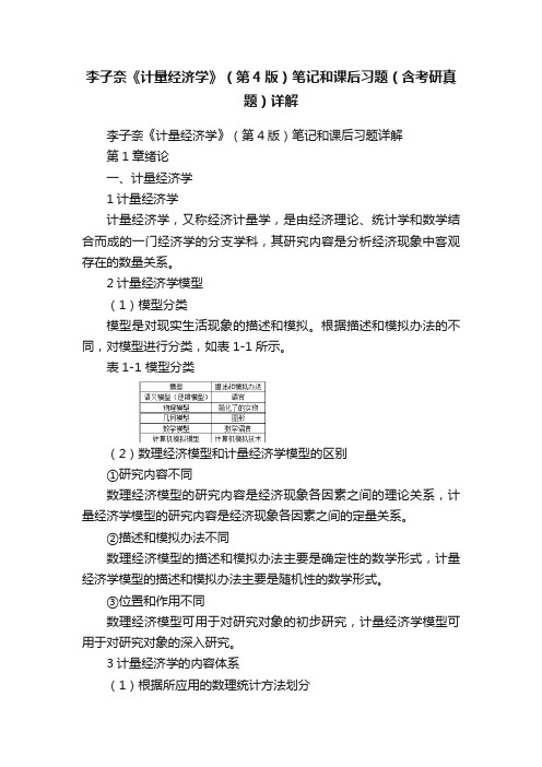
2.10(iii) From (2.57), Var(1ˆβ) = σ2/21()n i i x x =⎛⎫- ⎪⎝⎭∑. 由提示:: 21n i i x=∑ ≥21()n i i x x =-∑, and so Var(1β ) ≤ Var(1ˆβ). A more direct way to see this is to write(一个更直接的方式看到这是编写) 21()n ii x x =-∑ = 221()n i i x n x =-∑, which is less than21n i i x=∑unless x = 0.(iv)给定的c 2i x 但随着x 的增加, 1ˆβ的方差与Var(1β )的相关性也增加.0β小时1β 的偏差也小.因此, 在均方误差的基础上不管我们选择0β还是1β 要取决于0β,x ,和n 的大小 (除了 21n i i x=∑的大小).3.7We can use Table 3.2. By definition, 2β > 0, and by assumption, Corr(x 1,x 2) < 0. Therefore, there is anegative bias in 1β : E(1β ) < 1β. This means that, on average across different random samples, the simple regression estimator underestimates the effect of the training program. It is even possible that E(1β ) is negative even though 1β > 0. 我们可以使用表3.2。
根据定义,> 0,由假设,科尔(X1,X2)<0。
因此,有一个负偏压为:E ()<。
这意味着,平均在不同的随机抽样,简单的回归估计低估的培训计划的效果。
E (下),它甚至可能是负的,即使>0。
我们可以使用表格3.2。
根据定义,> 0,通过假设,柯尔(x1,x2)< 0。
因此,有一种负面的偏见:E()<。
这意味着,平均跨不同的随机样本,简单的回归估计低估了培训项目的效果。
甚至可能让E()是负的,尽管> 0。
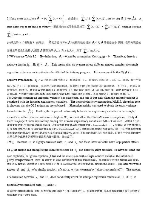
3.8 Only (ii), omitting an important variable, can cause bias, and this is true only when the omitted variable is correlated with the included explanatory variables. The homoskedasticity assumption, MLR.5, played no role in showing that the OLS estimators are unbiased. (Homoskedasticity was used to obtain the usual varianceformulas for the ˆjβ.) Further, the degree of collinearity between the explanatory variables in the sample, even if it is reflected in a correlation as high as .95, does not affect the Gauss-Markov assumptions. Only if there is a perfect linear relationship among two or more explanatory variables is MLR.3 violated. 只有3.8(ii),遗漏重要变量,会造成偏见确实是这样,只有当省略变量就与包括解释变量。
homoskedasticity 的假设,多元线性回归。
5,没有发挥作用在显示OLS 估计量是公正的。
(Homoskedasticity 是用来获取通常的方差公式。
)进一步,共线的程度解释变量之间的样品中,即使它是反映在尽可能高的相关性。
95年,不影响的高斯-马尔可夫假定。
只要有一个完美的线性关系在两个或更多的解释变量是多元线性回归。
三违反了。
3.9 (i) Because 1x is highly correlated with 2x and 3x , and these latter variables have large partial effectson y , the simple and multiple regression coefficients on 1x can differ by large amounts. We have not done thiscase explicitly, but given equation (3.46) and the discussion with a single omitted variable, the intuition is pretty straightforward. 因为 是高度相关,和这些后面的变量有很大部分影响y,简单和多元回归系数的差异可大量。
我们还没有做到,这种情况下显式,但鉴于方程(3.46)和以讨论单个变量遗漏,直觉是相当简单的。
(ii) Here we wouldexpect 1β and 1ˆβ to be similar (subject, of course, to what we mean by “almost uncorrelated”). The amount of correlation between 2x and 3x does not directly effect the multiple regression estimate on 1x if 1x is essentially uncorrelated with 2x and 3x .这里我们将期待和相似(主题,当然对我们所说的“几乎不相关的”)。
相关性的数量,但不会直接影响了多元回归估计如果本质上是不相关的和。
(iii) (iii) In this case we are (unnecessarily) introducing multicollinearity into the regression: 2x and 3x have small partial effects on y and yet 2x and 3x are highly correlated with 1x . Adding 2x and 3x likeincreases the standard error of the coefficient on 1x substantially, so se(1ˆβ) is likely to be much larger than se(1β ).在这种情况下我们(不必要的)引入重合放入回归:,有微小的部分影响,但y,是高度相关的。
添加和像增加标准错误的系数显著,所以se()可能会远远大于se()。
(iv) In this case, adding 2x and 3x will decrease the residual variance without causing much collinearity(because 1x is almost uncorrelated with 2x and 3x ), so we should see se(1ˆβ) smaller than se(1β ). The amount of correlation between 2x and 3x does not directly affect se(1ˆβ).在这种情况下,添加和将减少剩余方差,也没有引起共线(因为几乎是不相关的,),所以我们应该看到se()小于se()。
相关性的数量,但不会直接影响se()。
3.11 (i)1β < 0 because more pollution can be expected to lower housing values; note that 1β is the elasticityof price with respect to nox .2β is probably positive because rooms roughly measures the size of a house.(However, it does not allow us to distinguish homes where each room is large from homes where each room is small.) < 0,因为更多的污染可以预期较低的房屋价值;注意,价格弹性对氮氧化物。
可能是积极的因为房间粗略地度量大小的房子。
(然而,不允许我们自己去辨别的家中,每个房间都是大从家中,每个房间小。
)(ii) If we assume that rooms increases with quality of the home, then log(nox ) and rooms are negatively correlated when poorer neighborhoods have more pollution, something that is often true. We can use Table 3.2to determine the direction of the bias. If 2β > 0 and Corr(x 1,x 2) < 0, the simple regression estimator 1β has a downward bias. But because 1β < 0, this means that the simple regression, on average, overstates theimportance of pollution. [E(1β ) is more negative than 1β.]如果我们假设房间随质量的家里,然后日志(nox)和房间反比当没那么富裕的社区有更多的污染,这往往是正确的。
我们可以使用表3.2来确定方向的偏见。
如果> 0和柯尔(x1,x2)< 0,那么简单的(iii) This is what we expect from the typical sample based on our analysis in part (ii). The simple regression estimate, -1.043, is more negative (larger in magnitude) than the multiple regression estimate, -0.718. As those estimates are only for one sample, we can never know which is closer to 1β. But if this is a“typical” sample,1βis closer to -0.718. 这是我们期待的东西从典型的示例基于我们的分析部分(ii)。