第1章 Introductory Econometrics for Finance(金融计量经济学导论-东北财经大学 陈磊)
金融时间序列分析

《金融时间序列分析》讲义主讲教师:徐占东登录:徐占东《金融时间序列模型》参考教材:1.《金融时间序列的经济计量学模型》经济科学出版社米尔斯著2.《经济计量学手册》章节3.《Introductory Econometrics for Finance》 Chris Brooks 剑桥大学出版社4.《金融计量学:资产定价实证分析》周国富著北京大学出版社5.《金融市场的经济计量学》 Andrew lo等上海财经大学出版社6.《动态经济计量学》 Hendry著上海人民出版社7.《商业和经济预测中的时间序列模型》中国人民大学出版社弗朗西斯著8.《No Linear Econometric Modeling in Time series Analysis》剑桥大学出版社9.《时间序列分析》汉密尔顿中国社会科学出版社10.《高等时间序列经济计量学》陆懋祖上海人民出版社11.《计量经济分析》张晓峒经济科学出版社12.《经济周期的波动与预测方法》董文泉高铁梅著吉林大学出版社13.《宏观计量的若干前言理论与应用》王少平著南开大学出版社14.《协整理论与波动模型——金融时间序列分析与应用》张世英、樊智著清华大学出版社15.《协整理论与应用》马薇著南开大学出版社16.(NBER working paper)17.(Journal of Finance)18.(中国金融学术研究网) 教学目的:1)能够掌握时间序列分析的基本方法;2)能够应用时间序列方法解决问题。
教学安排1单变量线性随机模型:ARMA ; ARIMA; 单位根检验。
2单变量非线性随机模型:ARCH,GARCH系列模型。
3谱分析方法。
4混沌模型。
5多变量经济计量分析:V AR模型,协整过程;误差修正模型。
第一章引论第一节金融学简介一.金融学概论1.金融学:研究人们在不确定环境中进行资源最优配置的学科。
金融学的三个核心问题:资产时间价值,资产定价理论(资源配置系统)和风险管理理论。
第1章 INTERMEDIATE ECONOMETRICS-原版教材

Steps in Empirical Econometric Analysis
Specify hypothesis of interest in terms of the unknown parameters . Use econometric methods to estimate the parameters and formally test the hypothesizes of interest .
14
What can econometrics do for us?
Overall, we use econometrics to explain phenomena of economic nature, make policy recommendations and make forecasts about the future.
19
Steps in Empirical Econometric Analysis
Summary Econometrics is used in all applied economic fields to test economic theories, to inform government and private policy makers, and to predict economic time series. Sometimes, an econometric model is derived from a formal economic model, but in other cases, econometric models are based on informal economic reasoning and intuition. The goal of any econometric analysis is to estimate the parameters in the model and to test hypotheses about these parameters; the values and signs of the parameters determine the validity of an economic theory and the effects of certain policies.
第1章 Introductory Econometrics for Finance(金融计量经济学导论-东北财经大学 陈磊)

1.2 The Special Characteristics of Financial Data
• 宏观经济计量分析的数据问题:
• 小样本;测量误差与数据修正
1-13
• 金融数据的观测频率高,数据量大 • 金融数据的质量高
这些意味着可以采用更强有力的分析技术,研究结果也更 可靠。
• 金融数据包含很多噪音(noisy),更难以从随机 的和无关的变动中分辨出趋势和规律 • 通常不满足正态分布 • 高频数据经常包含反映市场运行方式的、但人们并 不感兴趣的其它模式(pattern) ,需要在建模时加以 考虑
1-15
Types of Data
• Problems that Could be Tackled Using a Time Series Regression - How the value of a country’s stock index has varied with that country’s macroeconomic fundamentals. - How the value of a company’s stock price has varied when it announced the value of its dividend payment. - The effect on a country’s currency of an increase in its interest rate • Cross-sectional data(截面数据) are data on one or more variables collected at a single point in time, e.g. - Cross-section of stock returns on the New York Stock Exchange - A sample of bond credit ratings for UK banks
Chapter 1 Introductory Economic Principles

Public Economics
Economics as a Social Science
中 山 大 学 政 务 学 院
• 经济学是一门科学。与其它科学一样,它由解释 (理论)和经验事实构成。其中,理论帮助我们 理解真实世界,并对真实世界作出正确的推测, 而经验事实则可以验证理论,也可能推翻它。 • 经济学研究诸如以下的问题:资本利得税的减少 会使股市上涨吗?提高关税会增加消费者的福利 吗?加长刑期会减少犯罪吗?离婚变得容易会提 高女性地位吗?高价(意味着销售量较低)战略 会比低价战略给企业带来更多利润吗?
表1.1 寻找社会问题的解决方案
问题
中 山 大 学 政 务 学 院
1、我国的钢铁生产者受到进
解决方案
对进口钢铁开征关税
可能的恶果
a.钢铁价格上升,使用钢铁的产业成本 增加,只好提高价格。 b.由于卖给我们的钢铁减少,外国人减 少购买我国的出口品。 a.屋主吝啬于维修保养。 b.较长期后,减少建造用来出租的房屋 a.雇主不太愿意雇佣女性。 b.厘定工资时增加了官僚和司法程序的 成本。
Public Economics
医学
全国本科
82
88
1,710
2,133
感谢08公政何敏仪同学提供
23
―经济人 (Economic man)‖
中 山 大 学 政 务 学 院
• ―经济人”这个术语经常用作贬义,含蓄地 批评经济推理。由于人们并不总是理性, 也并不总是自私,所以批评者就断言经济 学是建立在糟糕的基础之上的。但经济学 家并非主张理性和自私是放之四海而皆准 的绝对事实,他们更多地是以此构建研究 的前提假设。无论如何前提假设的有效性 是由其有用性来评定的。
口竞争的威胁。
introductory econometrics中文版目录

第1篇横截面数据的回归分析
第1章计量经济学的性质与经济数据
1.1 什么是计量经济学?
1.2 经验经济分析的步骤
1.3 经济数据的结构
1.4 计量经济分析中的因果关系和其他条件不变的概念
小结
关键术语
习题
计算机习题
第2章简单回归模型
第3章多元回归分析:估计
第4章多元回归分析:推断
第5章多元回归分析:OLS的渐近性
第6章多元回归分析:深入专题
第7章含有定性信息的多元回归分析:二值(或虚拟)变量第8章异方差性
第9章模型设定和数据问题的深入探讨
第2篇时间序列数据的回归分析
第10章时间序列数据的基本回归分析
第11章OLS用于时间序列数据的其他问题
第12章时间序列回归中的序列相关和异方差
第3篇高深专题讨论
第13章跨时横截面的混合:简单面板数据方法
第14章高深的面板数据方法
第15章工具变量估计与两阶段最小二乘法
第16章联立方程模型
第17章限值因变量模型和样本选择纠正
第18章时间序列高深专题
第19章一个经验项目的实施
附录A 基本数学工具
附录B 概率论基础
附录C 数理统计基础
附录D 矩阵代数概述
附录E 矩阵形式的线性回归模型附录F 各章问题解答
附录G 统计用表。
introductory econometrics for finance Chapter4_solutions
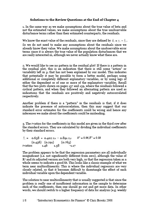
Solutions to the Review Questions at the End of Chapter 41. In the same way as we make assumptions about the true value of beta and not the estimated values, we make assumptions about the true unobservable disturbance terms rather than their estimated counterparts, the residuals.We know the exact value of the residuals, since they are defined by t t t y y uˆˆ-=. So we do not need to make any assumptions about the residuals since we already know their value. We make assumptions about the unobservable error terms since it is always the true value of the population disturbances that we are really interested in, although we never actually know what these are.2. We would like to see no pattern in the residual plot! If there is a pattern in the resi dual plot, this is an indication that there is still some “action” or variability left in y t that has not been explained by our model. This indicates that potentially it may be possible to form a better model, perhaps using additional or completely different explanatory variables, or by using lags of either the dependent or of one or more of the explanatory variables. Recall that the two plots shown on pages 157 and 159, where the residuals followed a cyclical pattern, and when they followed an alternating pattern are used as indications that the residuals are positively and negatively autocorrelated respectively.Another problem if there is a “pattern” in the residuals is that, if it does indicate the presence of autocorrelation, then this may suggest that our standard error estimates for the coefficients could be wrong and hence any inferences we make about the coefficients could be misleading.3. The t -ratios for the coefficients in this model are given in the third row after the standard errors. They are calculated by dividing the individual coefficients by their standard errors.t yˆ = 0.638 + 0.402 x 2t - 0.891 x 3t 89.0,96.022==R R (0.436) (0.291) (0.763)t -ratios 1.46 1.38 -1.17The problem appears to be that the regression parameters are all individually insignificant (i.e. not significantly different from zero), although the value of R 2 and its adjusted version are both very high, so that the regression taken as a whole seems to indicate a good fit. This looks like a classic example of what we term near multicollinearity. This is where the individual regressors are very closely related, so that it becomes difficult to disentangle the effect of each individual variable upon the dependent variable.The solution to near multicollinearity that is usually suggested is that since the problem is really one of insufficient information in the sample to determine each of the coefficients, then one should go out and get more data. In other words, we should switch to a higher frequency of data for analysis (e.g. weeklyinstead of monthly, monthly instead of quarterly etc.). An alternative is also to get more data by using a longer sample period (i.e. one going further back in time), or to combine the two independent variables in a ratio (e.g. x 2t / x 3t ).Other, more ad hoc methods for dealing with the possible existence of near multicollinearity were discussed in Chapter 4:- Ignore it: if the model is otherwise adequate, i.e. statistically and in terms of each coefficient being of a plausible magnitude and having an appropriate sign. Sometimes, the existence of multicollinearity does not reduce the t -ratios on variables that would have been significant without the multicollinearity sufficiently to make them insignificant. It is worth stating that the presence of near multicollinearity does not affect the BLUE properties of the OLS estimator – i.e. it will still be consistent, unbiased and efficient since the presence of near multicollinearity does not violate any of the CLRM assumptions 1-4. However, in the presence of near multicollinearity, it will be hard to obtain small standard errors. This will not matter if the aim of the model-building exercise is to produce forecasts from the estimated model, since the forecasts will be unaffected by the presence of near multicollinearity so long as this relationship between the explanatory variables continues to hold over the forecasted sample.- Drop one of the collinear variables - so that the problem disappears. However, this may be unacceptable to the researcher if there were strong a priori theoretical reasons for including both variables in the model. Also, if the removed variable was relevant in the data generating process for y , an omitted variable bias would result.- Transform the highly correlated variables into a ratio and include only the ratio and not the individual variables in the regression. Again, this may be unacceptable if financial theory suggests that changes in the dependent variable should occur following changes in the individual explanatory variables, and not a ratio of them.4. (a) The assumption of homoscedasticity is that the variance of the errors isconstant and finite over time. Technically, we write 2)(u t u Var σ=.(b ) The coefficient estimates would still be the “correct” ones (assuming that the other assumptions required to demonstrate OLS optimality are satisfied), but the problem would be that the standard errors could be wrong. Hence if we were trying to test hypotheses about the true parameter values, we could end up drawing the wrong conclusions. In fact, for all of the variables except the constant, the standard errors would typically be too small, so that we would end up rejecting the null hypothesis too many times.(c) There are a number of ways to proceed in practice, including- Using heteroscedasticity robust standard errors which correct for the problem by enlarging the standard errors relative to what they would havebeen for the situation where the error variance is positively related to one of the explanatory variables.- Transforming the data into logs, which has the effect of reducing the effect of large errors relative to small ones.5. (a) This is where there is a relationship between the i th and j th residuals. Recall that one of the assumptions of the CLRM was that such a relationship did not exist. We want our residuals to be random, and if there is evidence of autocorrelation in the residuals, then it implies that we could predict the sign of the next residual and get the right answer more than half the time on average!(b) The Durbin Watson test is a test for first order autocorrelation. The test is calculated as follows. You would run whatever regression you were interested in, and obtain the residuals. Then calculate the statistic()∑∑==--=T t t T t t t uuu DW 22221ˆˆˆYou would then need to look up the two critical values from the Durbin Watson tables, and these would depend on how many variables and how many observations and how many regressors (excluding the constant this time) you had in the model.The rejection / non-rejection rule would be given by selecting the appropriate region from the following diagram:(c) We have 60 observations, and the number of regressors excluding the constant term is 3. The appropriate lower and upper limits are 1.48 and 1.69 respectively, so the Durbin Watson is lower than the lower limit. It is thus clear that we reject the null hypothesis of no autocorrelation. So it looks like the residuals are positively autocorrelated.(d) t t t t t u x x x y +∆+∆+∆+=∆4433221ββββThe problem with a model entirely in first differences, is that once we calculate the long run solution, all the first difference terms drop out (as in the long run we assume that the values of all variables have converged on their own long run values so that y t = y t -1 etc.) Thus when we try to calculate the long run solution to this model, we cannot do it because there isn’t a long run solution to this model!(e) t t t t t t t t v X X x x x x y ++++∆+∆+∆+=∆---1471361254433221βββββββThe answer is yes, there is no reason why we cannot use Durbin Watson in this case. You may have said no here because there are lagged values of the regressors (the x variables) variables in the regression. In fact this would be wrong since there are no lags of the DEPENDENT (y ) variable and hence DW can still be used.6. t rt t t t t t t u x x x y x x y +++++∆+∆+=∆----471361251433221βββββββThe major steps involved in calculating the long run solution are to- set the disturbance term equal to its expected value of zero- drop the time subscripts- remove all difference terms altogether since these will all be zero by the definition of the long run in this context.Following these steps, we obtain373625410x x x y βββββ++++=We now want to rearrange this to have all the terms in x 2 together and so that y is the subject of the formula:344624541376251437362514)()(x x y x x y x x x y βββββββββββββββββ+---=+---=----=The last equation above is the long run solution.7. Ramsey’s RESET test is a test of whether the functional form of the regression is appropriate. In other words, we test whether the relationship between the dependent variable and the independent variables really should be linear or whether a non-linear form would be more appropriate. The test works by adding powers of the fitted values from the regression into a secondregression. If the appropriate model was a linear one, then the powers of the fitted values would not be significant in this second regression.If we fail Ramsey’s RESET test, then the easiest “solution” is probably to transform all of the variables into logarithms. This has the effect of turning a multiplicative model into an additive one.If this still fails, then we really have to admit that the relationship between the dependent variable and the independent variables was probably not linear after all so that we have to either estimate a non-linear model for the data (which is beyond the scope of this course) or we have to go back to the drawing board and run a different regression containing different variables.8. (a) It is important to note that we did not need to assume normality in order to derive the sample estimates of αand βor in calculating their standard errors. We needed the normality assumption at the later stage when we come to test hypotheses about the regression coefficients, either singly or jointly, so that the test statistics we calculate would indeed have the distribution (t or F) that we said they would.(b) One solution would be to use a technique for estimation and inference which did not require normality. But these techniques are often highly complex and also their properties are not so well understood, so we do not know with such certainty how well the methods will perform in different circumstances.One pragmatic approach to failing the normality test is to plot the estimated residuals of the model, and look for one or more very extreme outliers. These would be residuals that are much “bigger” (either very big and positive, or very big and negative) than the rest. It is, fortunately for us, often the case that one or two very extreme outliers will cause a violation of the normality assumption. The reason that one or two extreme outliers can cause a violation of the normality assumption is that they would lead the (absolute value of the) skewness and / or kurtosis estimates to be very large.Once we spot a few extreme residuals, we should look at the dates when these outliers occurred. If we have a good theoretical reason for doing so, we can add in separate dummy variables for big outliers caused by, for example, wars, changes of government, stock market crashes, changes in market microstructure (e.g. the “big bang” of 1986). The effect of the dummy variable is exactly the same as if we had removed the observation from the sample altogether and estimated the regression on the remainder. If we only remove observations in this way, then we make sure that we do not lose any useful pieces of information represented by sample points.9. (a) Parameter structural stability refers to whether the coefficient estimates for a regression equation are stable over time. If the regression is not structurally stable, it implies that the coefficient estimates would be different for some sub-samples of the data compared to others. This is clearly not what we want to find since when we estimate a regression, we are implicitly assuming that the regression parameters are constant over the entire sample period under consideration.(b) 1981M1-1995M12r t = 0.0215 + 1.491 r mt RSS =0.189 T =1801981M1-1987M10r t = 0.0163 + 1.308 r mt RSS =0.079 T =821987M11-1995M12r t = 0.0360 + 1.613 r mt RSS =0.082 T =98(c) If we define the coefficient estimates for the first and second halves of the sample as α1 and β1, and α2 and β2 respectively, then the null and alternative hypotheses areH 0 : α1 = α2 and β1 = β2and H 1 : α1 ≠ α2 or β1 ≠ β2(d) The test statistic is calculated asTest stat. =304.1524180*082.0079.0)082.0079.0(189.0)2(*)(2121=-++-=-++-k k T RSS RSS RSS RSS RSSThis follows an F distribution with (k ,T -2k ) degrees of freedom. F (2,176) = 3.05 at the 5% level. Clearly we reject the null hypothesis that the coefficients are equal in the two sub-periods.10. The data we have are1981M1-1995M12r t = 0.0215 + 1.491 R mt RSS =0.189 T =1801981M1-1994M12r t = 0.0212 + 1.478 R mt RSS =0.148 T =1681982M1-1995M12r t = 0.0217 + 1.523 R mt RSS =0.182 T =168First, the forward predictive failure test - i.e. we are trying to see if the model for 1981M1-1994M12 can predict 1995M1-1995M12.The test statistic is given by832.3122168*148.0148.0189.0*2111=--=--T k T RSS RSS RSSWhere T 1 is the number of observations in the first period (i.e. the period that we actually estimate the model over), and T 2 is the number of observations we are trying to “predict”. The test statistic follows an F -distribution with (T 2, T 1-k ) degrees of freedom. F (12, 166) = 1.81 at the 5% level. So we reject the null hypothesis that the model can predict the observations for 1995. We would conclude that our model is no use for predicting this period, and from a practical point of view, we would have to consider whether this failure is a result of a-typical behaviour of the series out-of-sample (i.e. during 1995), or whether it results from a genuine deficiency in the model.The backward predictive failure test is a little more difficult to understand, although no more difficult to implement. The test statistic is given by532.0122168*182.0182.0189.0*2111=--=--T k T RSS RSS RSSNow we need to be a little careful in our interpretation of what exactly are the “first” and “second” sample periods. It would be possible to define T 1 as always being the first sample period. But I think it easier to say that T 1 is always the sample over which we estimate the model (even though it now comes after the hold-out-sample). Thus T 2 is still the sample that we are trying to predict, even though it comes first. You can use either notation, but you need to be clear and consistent. If you wanted to choose the other way to the one I suggest, then you would need to change the subscript 1 everywhere in the formula above so that it was 2, and change every 2 so that it was a 1.Either way, we conclude that there is little evidence against the null hypothesis. Thus our model is able to adequately back-cast the first 12 observations of the sample.11. By definition, variables having associated parameters that are not significantly different from zero are not, from a statistical perspective, helping to explain variations in the dependent variable about its mean value. One could therefore argue that empirically, they serve no purpose in the fitted regression model. But leaving such variables in the model will use up valuable degrees of freedom, implying that the standard errors on all of the other parameters in the regression model, will be unnecessarily higher as a result. If the number of degrees of freedom is relatively small, then saving a couple by deleting two variables with insignificant parameters could be useful. On the other hand, if the number of degrees of freedom is already very large, the impact of these additional irrelevant variables on the others is likely to be inconsequential.12. An outlier dummy variable will take the value one for one observation in the sample and zero for all others. The Chow test involves splitting the sample into two parts. If we then try to run the regression on both the sub-parts butthe model contains such an outlier dummy, then the observations on that dummy will be zero everywhere for one of the regressions. For that sub-sample, the outlier dummy would show perfect multicollinearity with the intercept and therefore the model could not be estimated.。
IntroductiontoEconometrics

9
我们需要关于低STR的学区是否具有较高测 试成绩的数值证据——问题是怎么做?
1. 比较低 STR 的学区和高 STR 学区的平均测试成绩(“估 计”)
2. 检验原假设:2 种学区的平均测试成绩相同对备择假设:
它们不同 (“假设检验”)
3. 估计高 STR 学区和低 STR 学区之间差异的区间 (“置 信区间”)
1 nlarge
Ysmall Ylarge = nsmall
Yi
i1
– nlarge
Yi
i1
= 657.4 – 650.0
= 7.4
该差异在现实意义下大吗?
• 学区间的标准差 = 19.1 • 测试成绩分布的 60P和 75PP百分位数之差为 667.6 – 659.4 =
8.2 • 这个差异是否大到足以让家长或者学校委员会讨论学校
3
数据类型
• 截面数据 • 时间序列数据 • 面板数据
4
本课程的学习内容:
• 利用观测数据估计因果效应的方法 • 用于解决其它目的一些工具,如利用时间序列进行预测 • 集中于应用 ——理论仅仅只是用于理解采用这些方法的
原因 • 在练习中得到一些回归分析的实际操作经验
5
实证问题: 班级规模和教育产出 • 政策涉及的问题: 每班减少 1 人对测试成绩(或者其它后 果的度量)的效应有多大?每班减少 8 人呢? • 我们必须利用数据找出答案(在没有数据的情况下有其 它任何方法回答这个问题吗?)
2
如何利用数据度量因果效应
• 理想的状况是进行一项试验 • 为了估计班级规模对标准化测试成绩影响应该做怎样 的试验?
• 但大部分的实际状况是我们只有观测(非试验)数据 • 教育的收益 • 香烟价格 • 货币政策
微观经济学英文版第一章

理论和模型 Theories and Models
微观经济分析 Microeconomic Analysis
理论的演变 Evolving the Theory 检验和修正是经济科学发展的中心. Testing and refining theories is central to the development of the science of economics. 观察→检验→修正或完善,甚至是抛弃
Slide 5
关于教材的特点
特点二:内容组织合理、富有挑战性,令 人收益菲浅。
特点三:强调有用性,密切联系实际,穿插 80多个具体的案例分析,融合于全书之 中,帮助理解经济学基本理论和方法。
本书的两位作者都是著名经济学家,很多案 例都取材于计量经济学研究论文的内容,有 理有据。
Slide 6
本原理—加深理解在入门课程学过 的微观经济学
Slide 10
第一章 Chapter 1
绪论Preliminaries
概论微观经济学
稀缺、权衡取舍、经济模型与决策、竞争 性市场(I和II)与非竞争性市场(III和IV)的区 别
Slide 11
讨论的题目 Topics to be Discussed
Slide 30
实证分析 Positive Analysis
例如: For example: 进口配额对进口汽车有什么样的影响? What will be the impact of an import quota on foreign cars? 提高汽油税有什么样的影响? What will be the impact of an increase in the gasoline excise tax?
- 1、下载文档前请自行甄别文档内容的完整性,平台不提供额外的编辑、内容补充、找答案等附加服务。
- 2、"仅部分预览"的文档,不可在线预览部分如存在完整性等问题,可反馈申请退款(可完整预览的文档不适用该条件!)。
- 3、如文档侵犯您的权益,请联系客服反馈,我们会尽快为您处理(人工客服工作时间:9:00-18:30)。
1-4
Introductory Econometrics for Finance
Chris Brooks
1-5
作者简介
• Chris was formerly Professor of Finance at the ISMA Centre, University of Reading, where he also obtained his PhD and BA in Economics and Econometrics. • His areas of research interest include econometric modelling and forecasting, risk measurement, asset management, and property finance. • He has published over sixty articles in leading academic and practitioner journals, including the Journal of Business, the Journal of Banking and Finance, Journal of Empirical Finance, Oxford Bulletin and Economic Journal. • Chris is Associate Editor of several journals, including the International Journal of Forecasting.
1-14
1.3 Types of Data
• There are 3 types of data : 1. Time series data 2. Cross-sectional data 3. Panel data, a combination of 1. & 2. • The data may be quantitative (e.g. exchange rates, stock prices), or qualitative (e.g. day of the week). • Examples of time series data Series Frequency GNP or unemployment monthly, or quarterly government budget deficit annually money supply weekly value of a stock market index as transactions occur
1-17
1.4 Returns in Financial Modelling
• It is preferable not to work directly with asset prices, so we usually convert the raw prices into a series of returns. * There are two ways to do this: Simple returns or log returns
1. Testing whether financial markets are weak-form informationally efficient.(根据资产价格的历史数据检验资 产收益的可预测性) 2. Testing whether the CAPM or APT represent superior models for the determination of returns on risky assets. 3. Measuring and forecasting the volatility of bond returns. 4. Explaining the determinants of bond credit ratings used by the ratings agencies. 5. Modelling long-term relationships between prices and exchange rates
– 为金融市场的研究者提供从事金融时间序列的经验分析所必需的技术
• J.Y.Campbell et al.,1997, The Econometrics of Financial Market;《金融市场计量经济学》,上海财经大学出版社, 2003年。
– 专门介绍和论述股票市场、衍生证券、固定收入证券等方面的实证分析 方法和理论前沿。
1-1
金融计量经济学导论
讲授:陈 磊
电话:84712508 E-mail: chenlei@
1-2
学习要求与建议
• • • • • 作为理性人,应追求课堂收益最大化 课堂讲授+课下自学(最好课前预习) 阅读参考书 及时做习题 熟悉相关软件的使用
1-3
引
言
• 金融学的快速发展使它已成为一门相对独立的学科。 • 金融学“是一门具有高度实证性的科学”,“金融理 论与实证分析之间关系的密切程度是其他社会学科无 法相比的。” • 金融经济学家进行推断的基本方法是金融计量经济学, 即以模型为基础的统计推断。 • 课程目标:了解和掌握广泛应用于金融领域的现代经济 计量技术 • 缺少金融计量经济学方面的适当教科书
1-8
Chapter 1
Introduction
1-9
1.1 Introduction: The Nature and Purpose of Econometrics
• What is Econometrics? Literal meaning is “measurement in economics”. 对经济现象和经济关系的数量/计量分析 以经济理论和经济数据为依据,应用数学和统 计学的方法,通过建立数学模型来研究经济现象 及其变化规律的一门经济学科。 • Definition of financial econometrics: The application of statistical and mathematical techniques to problems in finance.
1-15
Types Data
• Problems that Could be Tackled Using a Time Series Regression - How the value of a country’s stock index has varied with that country’s macroeconomic fundamentals. - How the value of a company’s stock price has varied when it announced the value of its dividend payment. - The effect on a country’s currency of an increase in its interest rate • Cross-sectional data(截面数据) are data on one or more variables collected at a single point in time, e.g. - Cross-section of stock returns on the New York Stock Exchange - A sample of bond credit ratings for UK banks
1-12
Examples of the kind of problems that may be solved by an Econometrician
6. Testing the hypothesis that earnings or dividend
announcements have no effect on stock prices. 7. Testing whether spot or futures markets react more rapidly to news. 8.Forecasting the correlation between the returns to the stock indices of two countries.
• e.g. the daily prices of a number of blue chip stocks over two years.
• It is common to denote each observation by the letter t and the total number of observations by T for time series data, and to to denote each observation by the letter i and the total number of observations by N for cross-sectional data.
1-16
Types of Data and Notation
• Problems that Could be Tackled Using a Cross-Sectional Regression - The relationship between company size and the return to investing in its shares - The relationship between a country’s GDP level and the probability that the government will default on its sovereign debt. (主权债务) • Panel Data (平行数据,面板数据)has the dimensions of both time series and cross-sections,