Introductory Econometrics for Finance习题答案1

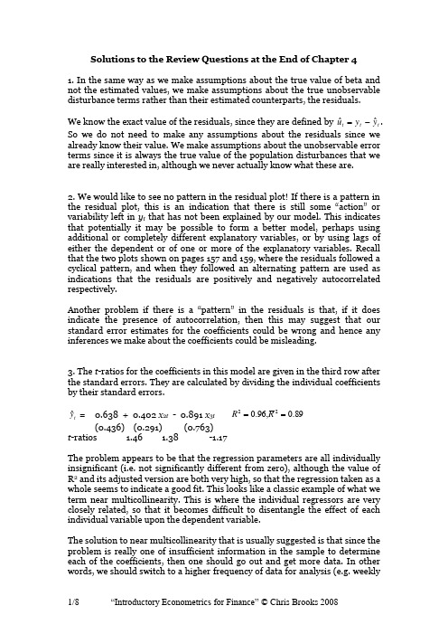
Solutions to the Review Questions at the End of Chapter 31. A list of the assumptions of the classical linear regression model’s disturbance terms is given in Box 3.3 on p56 of the book.We need to make the first four assumptions in order to prove that the ordinary least squares estimators of αand βare “best”, that is to prove that they have minimum variance among the class of linear unbiased estimators. The theorem that proves that OLS estimators are BLUE (provided the assumptions are fulfilled) is known as the Gauss-Markov theorem. If these assumptions are violated (which is dealt with in Chapter 4), then it may be that OLS estimators are no longer unbiased or “efficient”. That is, they may be inaccurate or subject to fluctuations between samples.We needed to make the fifth assumption, that the disturbances are normally distributed, in order to make statistical inferences about the population parameters from the sample data, i.e. to test hypotheses about the coefficients. Making this assumption implies that test statistics will follow a t-distribution (provided that the other assumptions also hold).2. If the models are linear in the parameters, we can use OLS.(1) Yes, can use OLS since the model is the usual linear model we have been dealing with.(2) Yes. The model can be linearised by taking logarithms of both sides and by rearranging. Although this is a very specific case, it has sound theoretical foundations (e.g. the Cobb-Douglas production function in economics), and it is the case that many relationships can be “approximately” linearised by taking logs of the variables. The effect of taking logs is to reduce the effect of extreme values on the regression function, and it may be possible to turn multiplicative models into additive ones which we can easily estimate.(3) Yes. We can estimate this model using OLS, but we would not be able to obtain the values of both β and γ, but we would obtain the value of these two coefficients multiplied together.(4) Yes, we can use OLS, since this model is linear in the logarithms. For those who have done some economics, models of this kind which are linear in the logarithms have the interesting property that the coefficients (αand β) can be interpreted as elasticities.5. Yes, in fact we can still use OLS since it is linear in the parameters. If we make a substitution, say Q t = X t Z t, then we can run the regression:y t = α +βQ t + u t as usual.So, in fact, we can estimate a fairly wide range of model types using these simple tools.3. The null hypothesis is that the true (but unknown) value of beta is equal to one, against a one sided alternative that it is greater than one:H0 : β = 1H1 : β > 1The test statistic is given by 682.20548.01147.1)ˆ(*ˆstat test =-=-=βββSE We want to compare this with a value from the t -table with T -2 degrees of freedom, where T is the sample size, and here T -2 =60. We want a value with 5% all in one tail since we are doing a 1-sided test. The critical t-value from the t -table is 1.671:The value of the test statistic is in the rejection region and hence we can reject the null hypothesis. We have statistically significant evidence that this security has a beta greater than one, i.e. it is significantly more risky than the market as a whole.4. We want to use a two-sided test to test the null hypothesis that shares in Chris Mining are completely unrelated to movements in the market as a whole. In other words, the value of beta in the regression model would be zero so that whatever happens to the value of the market proxy, Chris Mining would be completely unaffected by it.The null and alternative hypotheses are therefore:H 0 : β = 0H 1 : β ≠ 0The test statistic has the same format as before, and is given by: 150.1186.00214.0)(*ˆstat test =-=-=βββSE We want to find a value from the t -tables for a variable with 38-2=36 degrees of freedom, and we want to look up the value that puts 2.5% of the distribution in each tail since we are doing a two-sided test and we want to have a 5% size of test over all.Confidence intervals are almost invariably 2-sided, unless we are told otherwise (which we are not here), so we want to look up the values which put 2.5% in the upper tail and 0.5% in the upper tail for the 95% and 99% confidence intervals respectively. The 0.5% critical values are given as follows for a t-distribution with T-2=38-2=36 degrees of freedom:The confidence interval in each case is thus given by(0.214±0.186*2.03) for a 95% confidence interval, which solves to (-0.164,0.592) and(0.214±0.186*2.72) for a 99% confidence interval, which solves to (-0.292,0.720) There are a couple of points worth noting.First, one intuitive interpretation of an X% confidence interval is that we are X% sure that the true value of the population parameter lies within the interval. So we are 95% sure that the true value of beta lies within the interval (-0.164,0.592) and we are 99% sure that the true population value of beta lies within (-0.292,0.720). Thus in order to be more sure that we have the true vale of beta contained in the interval, i.e. as we move from 95% to 99% confidence, the interval must become wider.The second point to note is that we can test an infinite number of hypotheses about beta once we have formed the interval. For example, we would not reject the null hypothesis contained in the last question (i.e. that beta = 0), since that value of beta lies within the 95% and 99% confidence intervals. Would we reject or not reject a null hypothesis that the true value of beta was 0.6? At the 5% level, we should have enough evidence against the null hypothesis to reject it, since 0.6 is not contained within the 95% confidence interval. But at the 1% level, we would no longer have sufficient evidence to reject the null hypothesis, since 0.6 is now contained within the interval. Therefore we should always if possible conduct some sort of sensitivity analysis to see if our conclusions are altered by (sensible) changes in the level of significance used.6. It can be proved that a t-distribution is just a special case of the more general F-distribution. The square of a t-distribution with T-k degrees of freedom will be identical to an F-distribution with (1,T-k) degrees of freedom. But remember that if we use a 5% size of test, we will look up a 5% value for the F-distribution because the test is 2-sided even though we only look in one tail of the distribution. We look up a 2.5% value for the t-distribution since the test is 2-tailed.Examples at the 5% level from tablesT-k F critical value t critical value20 4.35 2.0940 4.08 2.0260 4.00 2.00120 3.92 1.987. We test hypotheses about the actual coefficients, not the estimated values. We want to make inferences about the likely values of the population parameters (i.e. to test hypotheses about them). We do not need to test hypotheses about the estimated values since we know exactly what our estimates are because we calculated them!8. (i) H0 : β3 = 2We could use an F- or a t- test for this one since it is a single hypothesis involving only one coefficient. We would probably in practice use a t-test since it iscomputationally simpler and we only have to estimate one regression. There is one restriction.(ii) H0 : β3 + β4 = 1Since this involves more than one coefficient, we should use an F-test. There is one restriction.(iii) H0 : β3 + β4 = 1 and β5 = 1Since we are testing more than one hypothesis simultaneously, we would use an F-test. There are 2 restrictions.(iv) H0 : β2 =0 and β3 = 0 and β4 = 0 and β5 = 0As for (iii), we are testing multiple hypotheses so we cannot use a t-test. We have 4 restrictions.(v) H0 : β2β3 = 1Although there is only one restriction, it is a multiplicative restriction. We therefore cannot use a t-test or an F-test to test it. In fact we cannot test it at all using the methodology that has been examined in this chapter.9. THE regression F-statistic would be given by the test statistic associated with hypothesis iv) above. We are always interested in testing this hypothesis since it tests whether all of the coefficients in the regression (except the constant) are jointly insignificant. If they are then we have a completely useless regression, where none of the variables that we have said influence y actually do. So we would need to go back to the drawing board!The alternative hypothesis is:H1 : β2≠ 0 or β3≠ 0 or β4≠ 0 or β5≠ 0Note the form of the alterna tive hypothesis: “or” indicates that only one of the components of the null hypothesis would have to be rejected for us to reject the null hypothesis as a whole.10. The restricted residual sum of squares will always be at least as big as the unrestricted residual sum of squares i.e.RRSS ≥ URSSTo see this, think about what we were doing when we determined what the regression parameters should be: we chose the values that minimised the residual sum of squares. We said that OLS would provide the “best” pa rameter values given the actual sample data. Now when we impose some restrictions on the model, so that they cannot all be freely determined, then the model should not fit as well as it did before. Hence the residual sum of squares must be higher once we have imposed the restrictions, otherwise the parameter values that OLS chose originally without the restrictions could not be the best.In the extreme case (very unlikely in practice), the two sets of residual sum of squares could be identical if the restrictions were already present in the data, so that imposing them on the model would yield no penalty in terms of loss of fit.11. The null hypothesis is: H0 : β3 + β4 = 1 and β5 = 1The first step is to impose this on the regression model:y t = β1 + β2x2t + β3x3t + β4x4t + β5x5t + u t subject to β3 + β4 = 1 and β5 = 1.We can rewrite the first part of the restriction as β4 = 1 - β3Then rewrite the regression with the restriction imposedy t = β1 + β2x2t + β3x3t+ (1-β3)x4t + x5t + u twhich can be re-writteny t = β1 + β2x2t + β3x3t + x4t - β3x4t + x5t + u tand rearranging(y t – x4t– x5t ) = β1+ β2x2t + β3x3t - β3x4t + u t(y t– x4t– x5t) = β1 + β2x2t + β3(x3t–x4t)+ u tNow create two new variables, call them P t and Q t:P t= (y t - x3t - x4t)Q t = (x2t -x3t)We can then run the linear regression:P t= β1 + β2x2t + β3Q t+ u t ,which constitutes the restricted regression model.The test statistic is calculated as ((RRSS-URSS)/URSS)*(T-k)/mIn this case, m=2, T=96, k=5 so the test statistic = 5.704. Compare this to an F-distribution with (2,91) degrees of freedom, which is approximately 3.10. Hence we reject the null hypothesis that the restrictions are valid. We cannot impose these restrictions on the data without a substantial increase in the residual sum of squares. 12. r i = 0.080 + 0.801S i + 0.321MB i + 0.164PE i - 0.084BETA i(0.064) (0.147) (0.136) (0.420) (0.120)1.25 5.452.36 0.390 -0.700The t-ratios are given in the final row above, and are in italics. They are calculated by dividing the coefficient estimate by its standard error. The relevant value from the t-tables is for a 2-sided test with 5% rejection overall. T-k = 195; t crit = 1.97. The null hypothesis is rejected at the 5% level if the absolute value of the test statistic is greater than the critical value. We would conclude based on this evidence that only firm size and market to book value have a significant effect on stock returns.If a stock’s beta increases from 1 t o 1.2, then we would expect the return on the stock to FALL by (1.2-1)*0.084 = 0.0168 = 1.68%This is not the sign we would have expected on beta, since beta would be expected to be positively related to return, since investors would require higher returns as compensation for bearing higher market risk.We would thus consider deleting the price/earnings and beta variables from the regression since these are not significant in the regression - i.e. they are not helping much to explain variations in y. We would not delete the constant term from the regression even though it is insignificant since there are good statistical reasons for its inclusion.。