a bistatic point target reference spectrum for general bistatic sar processing
安华高光纤模块选型

1x4 VCSEL Array
Din[4:1][p/n] (8) SCL SDA ModSelL LPMode ModPresL ResetL IntL Dout[4:1][p/n] (8) Electrical Interface
TX Input Buffer 4 Channels
Laser Driver 4 Channels
Optical Interface
Control
Diagnostic Monitors 1x4 PIN Array
RX Output Buf
Figure 1. Transceiver Block Diagram
Transmitter
The optical transmitter portion of the transceiver (see Figure 1) incorporates a 4-channel VCSEL (Vertical Cavity Surface Emitting Laser) array, a 4-channel input buffer and laser driver, diagnostic monitors, control and bias blocks. The transmitter is designed for IEC-60825 and CDRH eye safety compliance; Class 1M out of the module. The Tx Input Buffer provides CML compatible differential inputs presenting a nominal differential input impedance of 100 Ohms. AC coupling capacitors are located inside the QSFP+ module and are not required on the host board. For module control and interrogation, the control interface (LVTTL compatible) incorporates a Two Wire Serial (TWS) interface of clock and data signals. Diagnostic monitors for VCSEL bias, module temperature, and module power supply voltage are implemented and results are available through the TWS interface. Alarm and warning thresholds are established for the monitored attributes. Flags are set and interrupts generated when the attributes are outside the thresholds. Flags are also set and interrupts generated for loss of input signal (LOS) and transmitter fault conditions. All flags are latched and will remain set even if the condition initiating the latch clears and operation resumes. All interrupts can be masked and flags are reset by reading the appropriate flag register. The optical output will squelch for loss of input signal unless squelch is disabled. Fault detection or channel deactivation through the TWS interface will disable the channel. Status, alarm/warning and fault information are available via the TWS interface. To reduce the need for polling, the hardware interrupt signal is provided to inform hosts of an assertion of alarm, warning, LOS and/ or Tx fault.
淼田电子有限公司LQG15HH系列芯片电感说明书

SpecNo.JELF243B-9101H-01 P.1 / 11Reference OnlyCHIP COIL (CHIP INDUCTORS) LQG15HH □□□□02DMurata Standard REFERENCE SPECIFICATION [AEC-Q200]1.ScopeThis reference specification applies to LQG15HH series Chip coil (Chip Inductors) for Automotive Electoronics based on AEC-Q200.2.Part Numbering(ex) LQ G 15 H H 1N0 S 0 2 DProduct ID Struture Dimension Applications Category Inductance Tolerance Features Electrode Pakaging(L ×W) and for Automotive D:TapingCharacteristics Electoronics3.Rating・Operating Temperature Range. –55°C to +125°C ・Storage Temperature Range. –55°C to +125°CCustomer Part Number MURATAPart NumberInductance (nH) ToleranceQ(min.)DC Resistance (Ω max. ) Self ResonantFrequency (MHz min. )Rated Current (mA)ESD Rank 1C:1kV(*1)(refer to below comment)LQG15HH1N0B02D1.0B:±0.1nHC:±0.2nH S:±0.3nH8 0.07 10000 10001CLQG15HH1N0C02D LQG15HH1N0S02D LQG15HH1N1B02D1.1 6000 LQG15HH1N1C02DLQG15HH1N1S02D LQG15HH1N2B02D 1.2 LQG15HH1N2C02D LQG15HH1N2S02DLQG15HH1N3B02D1.3 LQG15HH1N3C02DLQG15HH1N3S02D LQG15HH1N5B02D1.5 LQG15HH1N5C02DLQG15HH1N5S02D LQG15HH1N6B02D 1.6 LQG15HH1N6C02D LQG15HH1N6S02D LQG15HH1N8B02D 1.8 0.08 950LQG15HH1N8C02D LQG15HH1N8S02DLQG15HH2N0B02D2.0 0.09 900LQG15HH2N0C02DLQG15HH2N0S02DLQG15HH2N2B02D 2.2 LQG15HH2N2C02D LQG15HH2N2S02D LQG15HH2N4B02D2.4 0.11 850 LQG15HH2N4C02DLQG15HH2N4S02D LQG15HH2N7B02D 2.7 0.12 800 LQG15HH2N7C02D LQG15HH2N7S02D LQG15HH3N0B02D 3.0 0.125LQG15HH3N0C02D LQG15HH3N0S02DLQG15HH3N3B02D3.3 LQG15HH3N3C02DLQG15HH3N3S02D LQG15HH3N6B02D3.6 0.14 750 LQG15HH3N6C02DLQG15HH3N6S02DCustomer Part Number MURATAPart NumberInductance (nH) ToleranceQ(min.)DC Resistance (Ω max. ) Self ResonantFrequency(MHz min. )RatedCurrent(mA)ESD Rank 1C:1kV(*1)(refer to below comment)LQG15HH3N9B02D3.9 B:±0.1nHC:±0.2nHS:±0.3nH8 0.14 6000 7501CLQG15HH3N9C02DLQG15HH3N9S02DLQG15HH4N3B02D 4.3 LQG15HH4N3C02D LQG15HH4N3S02D LQG15HH4N7B02D 4.7 0.16 700LQG15HH4N7C02D LQG15HH4N7S02DLQG15HH5N1B02D5.1 0.18 5300 650LQG15HH5N1C02DLQG15HH5N1S02DLQG15HH5N6B02D5.6 4500 LQG15HH5N6C02DLQG15HH5N6S02D LQG15HH6N2B02D6.2 0.20 600LQG15HH6N2C02DLQG15HH6N2S02DLQG15HH6N8G02D6.8 G:±2%H:±3%J:±5%0.22 LQG15HH6N8H02DLQG15HH6N8J02D LQG15HH7N5G02D 7.5 0.24 4200 550LQG15HH7N5H02D LQG15HH7N5J02DLQG15HH8N2G02D 8.2 3700 LQG15HH8N2H02D LQG15HH8N2J02DLQG15HH9N1G02D 9.1 0.26 3400500LQG15HH9N1H02D LQG15HH9N1J02DLQG15HH10NG02D10 LQG15HH10NH02D LQG15HH10NJ02D LQG15HH12NG02D12 0.28 3000 LQG15HH12NH02DLQG15HH12NJ02DLQG15HH15NG02D15 0.32 2500 450 LQG15HH15NH02DLQG15HH15NJ02D LQG15HH18NG02D18 0.36 2200 400 LQG15HH18NH02DLQG15HH18NJ02D LQG15HH22NG02D 22 0.42 1900 350 LQG15HH22NH02D LQG15HH22NJ02D LQG15HH27NG02D 27 0.46 1700 LQG15HH27NH02D LQG15HH27NJ02D LQG15HH33NG02D33 0.58 1600 LQG15HH33NH02DLQG15HH33NJ02D LQG15HH39NG02D39 0.65 1200 300 LQG15HH39NH02DLQG15HH39NJ02DCustomer Part Number MURATAPart NumberInductance (nH) Tolerance Q(min.) DC Resistance (Ω max. ) Self Resonant Frequency (MHz min. )Rated Current (mA)ESD Rank 1C:1kV(*1)(refer to below comment)LQG15HH47NG02D 47 G:±2%H:±3%J:±5%8 0.72 1000 3001CLQG15HH47NH02D LQG15HH47NJ02DLQG15HH56NG02D 56 0.82 800 250LQG15HH56NH02D LQG15HH56NJ02DLQG15HH68NG02D68 0.92 LQG15HH68NH02DLQG15HH68NJ02D LQG15HH82NG02D82 1.20 700 200 LQG15HH82NH02DLQG15HH82NJ02D LQG15HHR10G02D100 1.25 600 LQG15HHR10H02DLQG15HHR10J02DLQG15HHR12G02D120 1.30 LQG15HHR12H02DLQG15HHR12J02DLQG15HHR15G02D 150 2.99 550 150LQG15HHR15H02D LQG15HHR15J02DLQG15HHR18G02D 180 3.38 500 LQG15HHR18H02D LQG15HHR18J02D LQG15HHR22G02D 220 3.77 450 120 LQG15HHR22H02D LQG15HHR22J02D LQG15HHR27G02D270 4.94 400 110 LQG15HHR27H02DLQG15HHR27J02D(*1) Standard Testing Conditions《Unless otherwise specified 》 《In case of doubt 》Temperature : Ordinary Temperature / 15°C to 35°C Temperature: 20°C ± 2°CHumidity :Ordinary Humidity / 25%(RH) to 85%(RH) Humidity : 60%(RH) to 70%(RH) Atmospheric Pressure : 86kPa to 106 kPa4. Appearance and Dimensions■Unit Mass (Typical value)6.Q200 Requirement6.1.Performance (based on Table 5 for Magnetics(Inductors / Transformer)AEC-Q200 Rev.D issued June 1. 2010AEC-Q200 Murata Specification / Deviation No Stress TestMethod3 HighTemperatureExposure 1000hours at 125 deg CSet for 24hours at roomtemperature, then measured.Meet Table A after testing.Table A4 TemperatureCycling 1000cycles-40 deg C to +125 deg CSet for 24hours at roomtemperature,thenmeasured.Meet Table A after testing.7 Biased Humidity 1000hours at 85 deg C, 85%RHunpowered.Meet Table A after testing.8 Operational Life Apply 125 deg C 1000hoursSet for 24hours at roomtemperature, then measuredMeet Table A after testing.9 External Visual Visual inspection No abnormalities10 Physical Dimension Meet ITEM 4(Style and Dimensions)No defects12 Resistanceto Solvents PerMIL-STD-202Method 215Not ApplicableAppearance No damageInductanceChange(at 100MHz)Within ±10%AEC-Q200 Murata Specification / Deviation No Stress TestMethod13 Mechanical Shock Per MIL-STD-202Method 213Condition C : 100g’s(0.98N),6ms, Half sine, 12.3ft/sMeet Table A after testing.14 Vibration 5g's(0.049N) for 20 minutes,12cycles each of 3 oritentationsTest from 10-2000Hz.Meet Table A after testing.15 Resistanceto Soldering Heat No-heatingSolder temperature260C+/-5 deg CImmersion time 10sMeet Table A after testing.Pre-heating 150C +/-10 deg C, 60s to 90s17 ESD Per AEC-Q200-002 ESD Rank: refer to the Item3 (Rating).Meet Table A after testing18 Solderbility Per J-STD-002 Method b : Not Applicable90% of the terminations is to be soldered.19 ElectricalCharacterizationMeasured : Inductance No defects20 Flammability Per UL-94 Not Applicable21 Board Flex Epoxy-PCB(1.6mm)Deflection 2mm(min)Holding time 60s Meet Table B after testing.Table BAppearance No damage DCresistanceChangeWithin ±10%22 Terminal Strength Per AEC-Q200-006A force of 17.7Nfor 60s Murata Deviation Request: 5N No defects7.Specification of Packaging(in mm)7.2 Specification of Taping(1) Packing quantity (standard quantity)10,000 pcs. / reel(2) Packing MethodProducts shall be packed in the cavity of the base tape and sealed by top tape and bottom tape.(3) Sprocket holeThe sprocket holes are to the right as the tape is pulled toward the user.(4) Spliced pointBase tape and Top tape has no spliced point.(5) Missing components numberMissing components number within 0.1 % of the number per reel or 1 pc., whichever is greater,andare not continuous. The Specified quantity per reel is kept.0.8m ax.7.3 Pull StrengthTop tape5N min.Bottom tape7.4 Peeling off force of cover tapeSpeed of Peeling off 300mm/min Peeling off force0.1N to 0.6N(minimum value is typical)7.5 Dimensions of Leader-tape,Trailer and ReelThere shall be leader-tape ( top tape and empty tape) and trailer-tape (empty tape) as follows.7.6 Marking for reelCustomer part number, MURATA part number, Inspection number(*1) ,RoHS Marking(*2), Quantity etc ・・・*1) <Expression of Inspection No.> □□ OOOO ⨯⨯⨯(1) (2) (3)(1) Factory Code (2) Date First digit : Year / Last digit of yearSecond digit: Month / Jan. to Sep. → 1 to 9, Oct. to Dec. → O, N, D Third, Fourth digi : Day(3) Serial No.*2) <Expression of RoHS Marking> ROHS – Y (△)(1) (2)(1) RoHS regulation conformity parts. (2) MURATA classification number7.7 Marking for Outside package (corrugated paper box)Customer name, Purchasing order number, Customer part number, MURATA part number, RoHS Marking(*2) ,Quantity, etc ・・・7.8. Specification of Outer CaseOuter Case Dimensions(mm)Standard Reel Quantityin Outer Case (Reel)W D H 186 186 93 5* Above Outer Case size is typical. It depends on a quantity of an order.F165to 180degreeTop tape Bottom tapeBase tapeWDLabelH8. △!Caution8.1 Caution(Rating)Do not exceed maximum rated current of the product. Thermal stress may be transmitted to the product and short/open circuit of the product or falling off the product may be occurred.8.2 Fail-safe Be sure to provide an appropriate fail-safe function on your product to prevent a second damage that may becaused by the abnormal function or the failure of our product.8.3 Limitation of ApplicationsPlease contact us before using our products for the applications listed below which require especially high reliability for the prevention of defects which might directly cause damage to the third party's life, body or property.(1) Aircraft equipment (6) Transportation equipment (trains, ships, etc.) (2) Aerospace equipment (7) Traffic signal equipment(3) Undersea equipment (8) Disaster prevention / crime prevention equipment (4) Power plant control equipment (9) Data-processing equipment (5) Medical equipment (10) Applications of similar complexity and /or reliability requirements to the applications listed in the above9. NoticeProducts can only be soldered with reflow. This product is designed for solder mounting.Please consult us in advance for applying other mounting method such as conductive adhesive.9.1 Land pattern designinga 0.4b 1.4 to 1.5c 0.5 to 0.6(in mm)9.2 Flux, Solder・Use rosin-based flux.Don’t use highly acidic flux with halide content exceeding 0.2(wt)% (chlorine conversion value). Don’t use water-soluble flux. ・Use Sn-3.0Ag-0.5Cu solder.・Standard thickness of solder paste : 100μm to 150μm.Resist9.3 Reflow soldering conditions・Inductance value may be changed a little due to the amount of solder.So, the chip coil shall be soldered by reflow so that the solder volume can be controlled.・Pre-heating should be in such a way that the temperature difference between solder and product surface is limited to 150°C max. Cooling into solvent after soldering also should be in such a way that the temperature difference is limited to 100°C max.Insufficient pre-heating may cause cracks on the product, resulting in the deterioration of products quality. ・Standard soldering profile and the limit soldering profile is as follows.The excessive limit soldering conditions may cause leaching of the electrode and / or resulting in the deterioration of product quality.・Reflow soldering profileStandard Profile Limit Profile Pre-heating 150°C ~180°C 、90s ±30s Heating above 220°C 、30s ~60s above 230°C 、60s max. Peak temperature 245°C ±3°C 260°C,10s Cycle of reflow 2 times 2 times9.4 Reworking with soldering ironThe following conditions must be strictly followed when using a soldering iron.Pre-heating 150°C,1 min Tip temperature 350°C max. Soldering iron output 80W max. Tip diameter φ3mm max. Soldering time 3(+1,-0)sTime 2 timesNote :Do not directly touch the products with the tip of the soldering iron in order to prevent the crack on the products due to the thermal shock.9.5 Solder Volume・ Solder shall be used not to be exceed the upper limits as shown below.・ Accordingly increasing the solder volume, the mechanical stress to Chip is also increased. Exceeding solder volume may cause the failure of mechanical or electrical performance.1/3T ≦t ≦TT :thickness of product9.6 Mount ShockOver Mechanical stress to products at mounting process causes crack and electrical failure etc.Limit ProfileStandard Profile 90s±30s 230℃260℃245℃±3℃220℃30s~60s 60s max.180150Temp.(s)(℃)Time.9.7 Product’s locationThe following shall be considered when designing and laying out P.C.B.'s.(1) P.C.B. shall be designed so that products are not subjected to the mechanical stress due to warping the board.[Products direction ]Products shall be located in the sideways direction (Length:a <b) to the mechanical stress.(2) Components location on P.C.B. separation. It is effective to implement the following measures, to reduce stress in separating the board.It is best to implement all of the following three measures; however, implement as many measures as possible to reduce stress.Contents of MeasuresStress Level (1) Turn the mounting direction of the component parallel to the board separation surface. A > D *1 (2) Add slits in the board separation part.A >B (3) Keep the mounting position of the component away from the board separation surface. A > C*1 A > D is valid when stress is added vertically to the perforation as with Hand Separation.If a Cutting Disc is used, stress will be diagonal to the PCB, therefore A > D is invalid.(3) Mounting Components Near Screw HolesWhen a component is mounted near a screw hole, it may be affected by the board deflection that occurs during the tightening of the screw. Mount the component in a position as far away from the screw holes as possible.9.8 Cleaning ConditionsProducts shall be cleaned on the following conditions.(1) Cleaning temperature shall be limited to 60°C max.(40°C max for IPA.)(2) Ultrasonic cleaning shall comply with the following conditions with avoiding the resonance phenomenon at the mounted products and P.C.B.Power : 20 W / l max. Frequency : 28kHz to 40kHz Time : 5 min max.(3) Cleaner1. Alcohol type cleanerIsopropyl alcohol (IPA)2. Aqueous agentPINE ALPHA ST-100S(4) There shall be no residual flux and residual cleaner after cleaning. In the case of using aqueous agent, products shall be dried completely after rinse with de-ionized water in order to remove the cleaner. (5) Other cleaning Please contact us.〈Poor example 〉〈Good example 〉ba9.9 Resin coatingThe inductance value may change and/or it may affect on the product's performance due to highcure-stress of resin to be used for coating / molding products. So please pay your careful attention whenyou select resin.In prior to use, please make the reliability evaluation with the product mounted in your application set.9.10 Handling of a substrateAfter mounting products on a substrate, do not apply any stress to the product caused by bending ortwisting to the substrate when cropping the substrate, inserting and removing a connector from thesubstrate or tightening screw to the substrate.Excessive mechanical stress may cause cracking in the product.Bending Twisting9.11 Storage and Handing Requirements(1) Storage periodUse the products within 6 months after deliverd.Solderability should be checked if this period is exceeded.(2) Storage conditions・Products should be stored in the warehouse on the following conditions.Temperature: -10°C to 40°CHumidity: 15% to 85% relative humidity No rapid change on temperature and humidityDon't keep products in corrosive gases such as sulfur,chlorine gas or acid, or it may causeoxidization of electrode, resulting in poor solderability.・Products should be storaged on the palette for the prevention of the influence from humidity, dust and so on.・Products should be storaged in the warehouse without heat shock, vibration, direct sunlight and so on.・Products should be storaged under the airtight packaged condition.(3) Handling ConditionCare should be taken when transporting or handling product to avoid excessive vibration or mechanical shock.10.△!Note(1) Please make sure that your product has been evaluated in view of your specifications with our product being mounted to your product.(2) You are requested not to use our product deviating from the reference specifications.(3) The contents of this reference specification are subject to change without advance notice.Please approve our product specifications or transact the approval sheet for product specificationsbefore ordering.Reference OnlySpecNo.JELF243B-9101H-01 P.11 / 11。
HMC1161 MMIC VCO数据手册说明书

8.71 GHz to 9.55 GHz MMIC VCO with HalfFrequency Output Data Sheet HMC1161Rev. B Document FeedbackInformation furnished by Analog Devices is believed to be accurate and reliable. However, noresponsibility is assumed by Analog Devices for its use, nor for any infringements of patents or other rights of third parties that may result from its use. Specifications subject to change without notice. No license is granted by implication or otherwise under any patent or patent rights of Analog Devices. T rademarks and registered trademarks are the property of their respective owners. One Technology Way, P.O. Box 9106, N orwood, MA 02062-9106, U.S.A. Tel: 781.329.4700 ©2015 Analog Devices, Inc. All rights reserved. Technical Support FEATURESDual output frequency rangef OUT = 8.71 GHz to 9.55 GHzf OUT/2 = 4.355 GHz to 4.775 GHzOutput power (P OUT): 11 dBmSingle-sideband (SSB) phase noise: −115 dBc/Hz at 100 kHz No external resonator neededRoHS-compliant, 5 mm × 5 mm, 32-lead LFCSP: 25 mm² APPLICATIONSPoint to point and multipoint radiosTest equipment and industrial controlsVery small aperture terminals (VSATs) FUNCTIONAL BLOCK DIAGRAMNCNCNCNCGNDNCNCNC NCNCRFOUTNCV CCNCNCNCNC1RFOUT/21GND1NC1NC1NC1NC1NC5NC6NC7NC8NC9VTUNENC1NC2NC13382-1Figure 1.GENERAL DESCRIPTIONThe HMC1161 is a monolithic microwave integrated circuit (MMIC), voltage controlled oscillator (VCO) that integrates a resonator, a negative resistance device, and a varactor diode, and features a half frequency output. Because of the monolithic construction of the oscillator, the output power and phase noise performance are excellent over temperature.The output power is 11 dBm typical from a 5 V supply voltage. The VCO is housed in a RoHS-compliant LFCSP and requires no external matching components.HMC1161Data SheetRev. B | Page 2 of 11TABLE OF CONTENTSFeatures .............................................................................................. 1 Applications ....................................................................................... 1 Functional Block Diagram .............................................................. 1 General Description ......................................................................... 1 Revision History ............................................................................... 2 Specifications ..................................................................................... 3 Absolute Maximum Ratings ....................................................... 4 ESD Caution .................................................................................. 4 Pin Configuration and Function Descriptions ............................. 5 Interface Schematics .....................................................................6 Typical Performance Characteristics ..............................................7 Applications Information .................................................................9 Evaluation Printed Circuit Board (PCB) ..................................... 10 Bill of Materials ........................................................................... 10 Packaging and Ordering Information ......................................... 11 Outline Dimensions ................................................................... 11 Ordering Guide .. (11)REVISION HISTORY11/15—Rev. A to Rev. BChanges to Figure 3 and Figure 4 ................................................... 6 Changes to Ordering Guide, Note 1 (11)8/15—Revision A: Initial VersionThis Hittite Microwave Products data sheet has been reformatted to meet the styles and standards of Analog Devices, Inc.Data SheetHMC1161Rev. B | Page 3 of 11SPECIFICATIONST A = −40°C to +85°C, V CC = 5 V , unless otherwise noted. Table 1.Parameter Min Typ Max Unit Test Conditions/Comments FREQUENCY RangeOutput Frequency (f OUT ) 8.71 9.55 GHz Half Output Frequency (f OUT /2) 4.355 4.755 GHzDrift Rate 0.75 MHz/°CPulling 3.5 MHz p-p Pulling into a 2.0:1 voltage standing wave ratio (VSWR) Pushing2 MHz/V At VTUNE = 5 V OUTPUT POWER (P OUT )RFOUT 8 11 16 dBm RFOUT/20 4 8 dBmSupply Current (I CC ) 230 mA V CC = 4.75 V 200 250 300 mA V CC = 5.00 V270 mA V CC = 5.25 V HARMONICS, SUBHARMONICS 1/2 23 dBc 3/2 40 dBc Second 20 dBc Third 30 dBc TUNINGVoltage (VTUNE) 2 13 VSensitivity50 250 MHz/VTune Port Leakage Current 10 µA VTUNE = 13 V OUTPUT RETURN LOSS 2.5 dB SSB PHASE NOISE10 kHz Offset −90 −83 dBc/Hz 100 kHz Offset−115−109dBc/HzHMC1161Data SheetRev. B | Page 4 of 11ABSOLUTE MAXIMUM RATINGSTable 2.Parameter Rating V CC 5.5 V dc VTUNE0 V to 15 V TemperatureOperating −40°C to +85°C Storage−65°C to +150°C Nominal Junction (to Maintain 1 Million Hours Mean Time to Failure (MTTF))135°C Nominal Junction (T A = 85°C) 126.7°C Maximum Reflow Temperature (MSL3 Rating)260°C Thermal Resistance (Junction to Ground Paddle)31.4°C/W ESD Sensitivity (Human Body Model)Class 1AStresses at or above those listed under Absolute Maximum Ratings may cause permanent damage to the product. This is a stress rating only; functional operation of the product at these or any other conditions above those indicated in the operational section of this specification is not implied. Operation beyond the maximum operating conditions for extended periods may affect product reliability.ESD CAUTIONData SheetHMC1161Rev. B | Page 5 of 11PIN CONFIGURATION AND FUNCTION DESCRIPTIONSNC NC NC NC GND NC NC NC NCNC RFOUT NC V CC NC NC NC N C 1R F O U T /21G N D 1N C 1N C 1N C 1N C 1N C 5N C6N C 7N C 8N C 9V T U N E 0N C 1N C 2N C 13382-002NOTES1. NC = NO CONNECT. HOWEVER, THESE PINS CAN BECONNECTED TO RF/DC GROUND WITHOUT AFFECTING THE PERFORMANCE OF THE DEVICE.2. EXPOSED PAD. THE PACKAGE BOTTOM HAS AN EXPOSED METAL PAD THAT MUST BE CONNECTED TO RF/DC GROUND.Figure 2. Pin ConfigurationTable 3. Pin Function DescriptionsPin No.Mnemonic Description1 to 4, 6 to 10, 13 to 18, 20, 22 to 28, 30 to 32 NC No Connect. However, these pins can be connected to RF/dc ground without affecting the performance of the device.5, 11 GND Ground. These pins must be connected to RF/dc ground. 12 RFOUT/2 Half Frequency Output. This pin is ac-coupled. 19 RFOUT RF Output. This pin is ac-coupled. 21 V CC Supply Voltage (5 V).29 VTUNE Control Voltage and Modulation Input. The modulation bandwidth is dependent on the drive source impedance.EPExposed Pad. The package bottom has an exposed metal pad that must be connected to RF/dc ground.HMC1161Data SheetRev. B | Page 6 of 11INTERFACE SCHEMATICSRFOUT/213382-004Figure 3. RFOUT/2 InterfaceRFOUT13382-003Figure 4. RFOUT InterfaceV 13382-005Figure 5. V CC InterfaceVTUNE13382-006Figure 6. VTUNE Interface13382-007Figure 7. GND InterfaceData SheetHMC1161Rev. B | Page 7 of 11TYPICAL PERFORMANCE CHARACTERISTICS10.07.07.58.08.59.09.512345678910111213O U T P U T F R E Q U E N CY (G H z )TUNING VOLTAGE (V dc)13382-008Figure 8. Output Frequency vs. Tuning Voltage1602461014812012345678910111213O U T P U T P O WE R (d B m )TUNING VOLTAGE (V dc)13382-009Figure 9. Output Power vs. Tuning Voltage6000100200300400500012345678910111213S E N S I T I V I T Y(M H z /V )TUNING VOLTAGE (V dc)13382-010Figure 10. Sensitivity vs. Tuning Voltage300200220240210230250270290260280012345678910111213S U P P L Y C U R RE N T (m A )TUNING VOLTAGE (V dc)13382-011Figure 11. Supply Current (I CC ) vs. Tuning Voltage5.003.503.754.004.254.504.7512345678910111213R F O U T /2 O U T P U T F R E Q U E NC Y (G H z )TUNING VOLTAGE (V dc)13382-012Figure 12. RFOUT/2 Output Frequency vs. Tuning Voltage100241357968012345678910111213R F O U T /2 O U T P U T P O WE R (d B m )TUNING VOLTAGE (V dc)13382-013Figure 13. RFOUT/2 Output Power vs. Tuning VoltageHMC1161Data SheetRev. B | Page 8 of 11–70–120–110–100–115–105–95–85–75–90–8012345678910111213S S B P H A S E N O I S E (d B c /H z )TUNING VOLTAGE (V dc)13382-014Figure 14. SSB Phase Noise vs. Tuning Voltage–50–140–130–110–120–100–80–60–90–7010k100k 1M 10MS S B P H A S EN O I S E (d B c /H z )OFFSET FREQUENCY (Hz)13382-015Figure 15. SSB Phase Noise vs. Offset Frequency at VTUNE = 5 VData SheetHMC1161Rev. B | Page 9 of 11APPLICATIONS INFORMATIONThe HMC1161 serves as the local oscillator (LO) in microwave synthesizer applications. The primary applications are point-to-point microwave radios, military, radars, test and measurement, as well as industrial and medical equipment. The low phase noise allows higher orders of modulation and offers improved bit error rates in communication systems, whereas the linear, monotonic tuning sensitivity allows a stable loop filter design. The higher output power minimizes the gain required to drivesubsequent stages. The half frequency output reduces the input frequency to the prescaler without the addition of residual phase noise to the input of the phase-locked loop synthesizer.13382-016Figure 16. Typical Application DiagramHMC1161Data SheetRev. B | Page 10 of 11EVALUATION PRINTED CIRCUIT BOARD (PCB)13382-017Figure 17. Evaluation PCBThe circuit board used in an application uses RF circuit design techniques. Ensure that the signal lines have 50 Ω impedance and that the package ground leads and backside ground paddle are connected directly to the ground plane.Use a sufficient number of via holes to connect the top and bottom ground planes. The evaluation circuit board shown in Figure 17 is available from Analog Devices, Inc., upon request.BILL OF MATERIALSTable 4. Bill of Materials for the EV1HMC1161LP5Item DescriptionJ1 to J4 PCB mount SMA RF connectors J5, J6 2 mm dc headersC1 to C3 100 pF capacitors, 0402 package C41000 pF capacitor, 0402 package C5 to C7 2.2 μF tantalum capacitorsC8 0.01 μF capacitor, 0603 package U1 HMC1161 VCOPCB 1110225 evaluation board 21 Circuit board material is Rogers 4350.2Reference this number when ordering the complete evaluation PCB.Data SheetHMC1161Rev. B | Page 11 of 11PACKAGING AND ORDERING INFORMATIONOUTLINE DIMENSIONS03-04-2015-A0.081.000.90FOR PROPER CONNECTION OF THE EXPOSED PAD, REFER TO THE PIN CONFIGURATION AND FUNCTION DESCRIPTIONSSECTION OF THIS DATA SHEET.COMPLIANT TO JEDEC STANDARDS MO-220-VHHD-4.000000Figure 18. 32-Lead Lead Frame Chip Scale Package [LFCSP_VQ]5 mm × 5 mm Body, Very Thin Quad(HCP-32-1)Dimensions shown in millimeters1 The HMC1161LP5E and HMC1161LP5ETR are RoHS compliant parts.2See the Absolute Maximum Ratings section, Table 2. 3XXXX is a placeholder for the 4-digit lot number.©2015 Analog Devices, Inc. All rights reserved. Trademarks and registered trademarks are the property of their respective owners.D13382-0-11/15(B)/HMC1161。
In Search of the Dark Ages -- An Experimental Challenge
a r X i v :a s t r o -p h /0404241v 1 13 A p r 2004D RAFT VERSION F EBRUARY 2,2008Preprint typeset using L A T E X style emulateapj v.2/19/04IN SEARCH OF THE DARK AGES –AN EXPERIMENTAL CHALLENGEJ.B LAND -H AWTHORNAnglo-Australian Observatory,P.O.Box 296,Epping,NSW 2121,AustraliaANDP.E.J.N ULSEN 1Harvard-Smithsonian Center for Astrophysics,60Garden Street,Cambridge,MA 02138Draft version February 2,2008ABSTRACTMost direct source detections beyond z ∼7are likely to arise from wide-field narrowband surveys of Ly αemission in the J band.For this to be true,the Ly αemission must somehow escape from compact star-forming regions (CSR)presumably associated with massive haloes.Since the Ly αescape fraction is 10%from an emitting region of size ∼1kpc,these objects will be difficult to find and hard to detect,requiring ∼30–100hours at each telescope pointing on 8–10m telescopes.For CSR sources,existing large-format IR arrays are close to ideal in terms of their noise characteristics for conducting wide-field narrowband surveys where pixel sizes are 0.1′′or larger.However,we stress that Ly αcan also arise from external large-scale shocks (ELS)due to starburst winds,powered by CSRs,ploughing into gas actively accreting onto the dark halo.The winds effectively carry energy from the dense,dusty environment of a starburst into lower density regions,where the escape probability for Ly αphotons is greater.ELS emission is expected to be considerably more clumpy ( 100pc)than CSR emission.For ELS sources,IR arrays will need 1−2orders of magnitude improvement in dark current in order to detect dispersed clumpy emission within the environments of massive haloes.These sources require an IR camera with small pixels (∼0.01′′)and adaptive optics correction (e.g.,GSAOI on Gemini),and will therefore require a targetted observation of a Dark Age source identified by a wide-field survey.For either targetted or wide-field surveys,the deepest observations will be those where the pixel sampling is well matched to the size of the emitting regions.We show that there are only 3–4J-band windows [z =7.72,(8.22),8.79,9.37]suitable for observing the Dark Ages in Ly α;we summarize their cosmological properties in Table 1.Subject headings:cosmology;first stars;intergalactic medium;galaxies —high redshift1.INTRODUCTIONIn recent years,we have come to recognize that the ‘ion-ization epoch’may lie just beyond our current observational horizon (cf.Fan et al.2000,2003;Kneib et al.2004).Struc-ture formation models in CDM cosmologies appear to show that this epoch took place at z =7–12(Gnedin &Ostriker 1997;Haiman &Loeb 1998).Recent wide-angle polariza-tion measurements with WMAP (Kogut et al.2003)suggest the ionization epoch could have been well under way by z ∼17.However,this may conflict with the inferred high column densities in z ∼6quasars (e.g.,Wyithe &Loeb 2004).Since cosmic ionization requires only a tiny fraction of the primordial gas to be converted into stars or black holes (Loeb &Barkana 2001),it is possible to construct a wide range of scenarios (Bromm,Coppi &Larson 1999,2002;Nakamura &Umemura 2001;Abel,Bryan &Norman 2000,2002;Bromm &Larson 2004;Barkana &Loeb 2000;Wyithe &Loeb 2003;Haiman,Thoul &Loeb 1996;Fryer,Woosley &Heger 2001).Clearly,the first observa-tions of the Dark Ages will have a dramatic impact on our understanding of this new frontier.In conventional CDM simulations,CSR sources are associ-ated with the cores of massive haloes.Since the distribution of dense peaks collapsing out of an evolving Gaussian den-sity field is well constrained (Miralda-Escudé2003;Peacock 1999),bright CSR sources are expected to be rare.These will be difficult to find even with well optimized wide-field sur-veys which exploit large pixels (∼0.1′′).However,the num-1On leave from the University of Wollongongber of detectable sources above a given flux level at a fixed epoch is more uncertain.This requires a detailed understand-ing of how and when Ly αemission is produced,and how it manages to escape its immediate environment (Neufeld 1991;Haiman &Spaans 1999).Even the most optimistic calcula-tions (Baron &White 1987)show that Ly αdetections will be a major observational challenge on 8–10m telescopes.The possible discovery of a lensed candidate galaxy at z =10by Pellóet al.(2004)demonstrates the power of lensing to ex-tend our observational reach.However,the total number of sources accessible this way is limited by the small total vol-ume of the universe that is strongly magnified by foreground lenses.During the Dark Ages,gas accretion onto protogalactic cores must have been well under way.Galactic nuclei at the highest redshifts observed to date (z ∼5)exhibit solar metal-licities,and therefore appear to have undergone many cycles of star formation (Hamann &Ferland 1999).Most galaxy cores early in their evolution must have experienced starburst-driven winds.Early protogalactic winds will have carried large amounts of energy,with relatively low dust/metal con-tent,away from the complex circumnuclear environment (Desjacques et al.2004).In order to understand physical processes associated with the first sources,we will need to resolve the Ly αstructures.But,as we now show,detecting emission powered by outflows is a different experimental challenge from that posed by wide-field searches.22.THE Ly αCHALLENGE 2.1.Wind-scattered Ly αemissionThe difficulty of detecting Ly αduring the Dark Ages is em-phasized in recent simulations by the GALFORM consortium (Lacey et al.2004;Cole et al.2000).The GALFORM sim-ulations assume that all Ly αis produced by star formation,and that 10%escapes through the action of galactic winds.The simulations are adjusted so as to reproduce the Lyman-break and submillimetre galaxy number counts at presently observed wavelengths.Down to a limiting flux magnitude of f lim =3×10⁻¹⁹erg cm −2s −1,they predict only about ten sources per square arcmin will be observable across the entire redshift range corresponding to the J band.The flux limit is equivalent to a star formation rate of a few solar masses per year which is easily high enough to drive large-scale winds (Heckman 2003;Veilleux 2003).The most efficient mechanism for Ly αescape is scat-tering by neutral H entrained in an outflowing wind (Chen &Neufeld 1994).The best observed starburst galaxy M82reveals UV-scattered bicones along the minor axis (Courvoisier et al.1990;Blecha et al.1990)on a scale of 500pc to 1kpc.This corresponds to a spatial scale of 0.1–0.2′′at z ∼8.Thus wide-field searches of rare massive haloes will need to exploit pixels on this scale in order to find CSR sources.The scattering wind may be clumped but,as we dis-cuss below,the individual clumps are likely to fall below the detection limit.2.2.Wind-driven Ly αemissionWe now examine the likelihood that most of the Ly αis dis-tributed in small clumps which are cooling out of dissipating gas,and spread over a larger volume than Ly αarising directly from star forming regions.During the early stages of galaxy formation,collapse is likely to be comparable to star formation as a source of energy for the gas.Cold gas accumulated in the collapse of a small halo (Rees &Ostriker 1977)produces an initial burst of star formation.If the energy released into the nascent interstellar medium by star formation greatly exceeded that released in the collapse,then the bulk of the gas would be unbound from the young galaxy.On the other hand,the mechanical energy required to limit the initial burst of star formation is compa-rable to the binding energy of the gas,which is roughly the energy needed to significantly rearrange gas within a galaxy.Thus,if the burst of star formation is self-limiting,its feed-back cannot fall well short of the binding energy of the gas,i.e.,the energy released by the collapse.Since radiative cooling times of gas at the virial tempera-ture are much shorter than dynamical times in low mass pro-togalaxies,feedback can only be stored briefly as thermal en-ergy.Energy rapidly lost to radiation is ineffective as feed-back.Only feedback energy that is converted to kinetic (and later potential)energy can be effective in limiting star forma-tion on the dynamical timescale.Effective feedback needs to induce rapid large-scale flows,i.e.,winds,so we assume that the primary channel of feedback is through winds.This argu-ment requires a moderately high efficiency for the conversion of energy released by star formation into wind energy,but that is consistent with observations of starburst winds (e.g.,Strickland &Stevens 2000).If collapse and the initial burst of star formation make com-parable energy inputs to the ISM,we can estimate both using the spherical collapse model.To form a disk,gas must dissi-F IG .1.—Cooling width of a collapse shock at z =8.This shows the prod-uct of postshock cooling time and postshock speed as a function of the shock speed,for gas with a preshock electron density of 0.036cm −3and abundances of 0,0.1and 1solar (top to bottom).The cooling width is inversely propor-tional to preshock density.pate at least the vertical component of its velocity dispersion,i.e.,σ2/2per unit mass.For a dissipative collapse —one pro-ducing cold gas —the energy dissipated is several times this,so we use the estimate of σ2per unit mass dissipated by gas in the collapse.The time taken for a halo to virialize is roughly equal to its turn around time,i.e.,half of its collapse time,t c .If the energy dissipated in the collapse is dissipated in half of the virialization time,the dissipation rate 4M g σ2/t c ,where M g is the gas mass involved in the collapse.Dark energy is insignificant for collapse at z ∼8,so that themean density of a halo collapsing at t c is 3π/(Gt 2c ),giving thevirial radius for a halo of mass M as R =[GMt 2c /(4π2)]1/3.Treating the halo as an isothermal sphere (GM /R =2σ2),then gives σ2=0.5(2πGM /t c )2/3,so that σ≃53M 1/310km s −1,where the halo mass M =1010M 10M ⊙and t c =6.27×10⁸yr [z =8,in ΛCDM with (h ,Ωm ,ΩΛ)=(0.7,0.3,0.7)].Little Ly αcan be produced in the collapse unless the gas is heated over ∼104K,i.e.,unless σ 10km s −1,requiring halo masses ex-ceeding 108M ⊙.Using the baryon fraction determined by WMAP (f b =Ωb /Ωm ≃0.17;Spergel et al.2003)and assuming that all baryons are gaseous in the collapse,the dissipation rate in the gas during a collapse is P d ≃4f b M σ2/t c ≃2×1040M 5/310erg s −1.Instantaneous dissipation rates will show a significant spread about this value.The fraction emerging as Ly αphotons depends on the shock temperature and the fraction of photons that escape.Higher escape fractions are favoured by low optical depth and low abundances (low dust content).In standard ΛCDM,very few 1010M ⊙halos col-lapse before z =8(Cole et al.2000).While the fraction of Ly αphotons escaping from starbursts is small,a significant part of the energy carried off by galactic winds is ultimately likely to be dissipated in shocks.These are another potential source of Ly αphotons and,from above,the energy in the winds is comparable to that dissipated in the collapse.The winds effectively carry energy from the dense,dusty environment of a starburst into lower density regions,where the escape probability for Ly αphotons is greater.Star-burst wind speeds are high and not strongly dependent on the properties of the hosting halo.This means that if starbursts3 are triggered in halos smaller than108M⊙,then the terminat-ing shocks of galactic winds may produce Lyαalthough thecollapse shocks cannot.From above,the mean baryon density in a dissipationlesshalo collapsing at z=8is3πf b/(Gm H t2c)≃0.036cm−3,wherem H is the mass of hydrogen.Since dissipation significantlyincreases the density of the gas,the typical density of gas run-ning into shocks during a dissipative collapse can be some-what larger than this.The collapse is fairly chaotic and col-lapsing gas is likely to encounter several shocks beforefinallyreaching its destination.Provided that the effects of radia-tion transfer are not too significant,the depth of the emittingregion behind a radiative shock is approximately equal to the product of the postshock cooling time and velocity.In a strongshock,the gas density is increased by a factor of4,the speed is decreased by the same factor and the postshock temperature is T ps=3µm H v2s/(16k),where v s is the shock speed andµm H is the mean mass per particle.Fig.1shows the width of the postshock cooling region for a preshock electron density of 0.036cm−3,for metal abundances of0,0.1and1solar. Initially,the collapsing gasflow may be coherent on larger scales than the postshock cooling length in Fig.1.In that case, cooling shocked regions are sheetlike and emission is bright-est at caustics where we see folds in these sheets projected onto the sky.The cooling gas is subject to thermal and other instabilities that will generally cause it to fragment on about the scale of the cooling length.(Theflow into any further shocks is likely to be considerably more chaotic.)For haloes in the mass range of interest,the shock speeds in the collapse are,at most,100–200km s−1.In a pristine gas,the inferred size of cooling clumps is roughly100pc,or0.02′′at a red-shift of z∼8.The small size of the cooling region demands an infrared imager which utilizes small pixels(∼0.01′′)and adaptive optics correction.However,we point out that rapid winds from starbursts can produce significantly larger cooling regions.Since gas is compressed significantly in a dissipative col-lapse,the time scale for star formation in a clump of col-lapsed gas can be much shorter than the dynamical time of the collapsing system(∼108yr).Massive stars take only ∼106yr to produce supernovae,giving plenty of time for starbursts and their winds to get underway while other gas continues to collapse into the system.Interaction between infalling gas and starburst winds can lead to further shock-ing of both.This process is observed in M82where the out-flowing starburst-driven wind impinges directly on infalling gas at a radius of11kpc(Yun,Ho&Lo1994)producing observable Hαand x-ray emission(Devine&Bally1999; Lehnert,Heckman&Weaver1999).3.EXPECTED LyαSURFACE BRIGHTNESSWe now examine whether wind-powered Lyαemission in small clumps can be detected with an8m telescope using an adaptive optics imager with small pixels(0.02").We assume that the total energy released in Lyαat afixed star formation rate is comparable to what is generated in large-scale shocks driven by the starburst,and that this emission escapes without attenuation.As discussed in§2.2,this assumes a high con-version rate of the supernova energy into wind energy(e.g., Strickland&Stevens2000).From surveys of nearby dwarf galaxies(Martin2003; Veilleux2003),we adopt a wind radius of5kpc.At z∼8,the shock occurs at1′′radius and is barely re-solved.Naively,if the wind energy escapes along bipo-00.20.40.60.810.20.40.60.81F IG.2.—Filter profiles used in our GSAOI calculations.The Lorentzian profile(m=1)shown in black is the expected response of a highfinesse (N=40)tunablefilter.The green profile(m=2)is the low-costfilter option, the blue profile(m=3)is the high-costfilter option.lar cones,the Lyαsurface brightness will be increased by the decrease in solid angle compared to a spherical wind.This factor can be∼10since most winds appear to be highly collimated(Shopbell&Bland-Hawthorn1998; Sugai,Davies&Ward2003).However,this factor does not apply to a comparison with the expectedflux from a CSR, since the normal assumption is that the collimated wind ma-terial is what renders the central source visible.An escape fraction of10%assumed in the GALFORM simulations is the fraction of radiation which escapes along the bicones multi-plied by the fraction scattered in the wind.For wind-induced emission,in our model,the total power available is10f lim but this is now spread over many more pix-els.The surface brightness of the shock induced Lyαemission depends critically on how the bipolar shock surfaces are ori-ented with respect to the observer.If the bipolar wind lies in the plane of the sky,most of the emission is confined to limb-brightened arcs over an area of∼102pixels depending on the curvature of the shock surface.If the bipolar wind is directed at the observer,the projected radius of the shocked-induced nebula is half the intrinsic radius(60◦opening angle).Thus, theflux is now dispersed over an area of∼103pixels.Our expectation is that the Lyαflux per pixel will be an or-der of magnitude fainter in external large-scale shocks(ELS) compared to CSR emission in a large pixel survey(0.1").We believe that it will be important to reach thisflux level if we are to understand the nature and origin of the Lyαemission. We have assumed that essentially all of the Lyαemission es-capes its environs since it is produced in situ.But in the pres-ence of any diffuse intergalactic HI component at rest with the expanding universe,the shock surface must have a suffi-cient redshift in order for the Lyαemission to escape to the observer.We have already noted that CSR emission is rendered visi-ble through scattering by neutral H in the wind.From the lo-4TABLE1B ASIC COSMOLOGICAL PARAMETERS FOR THE FOUR DARK J-BANDWINDOWS.Wavelength(µm) 1.06 1.12 1.19 1.26 Redshift7.728.228.799.37 Time since Big Bang(Gyr)0.660.600.550.51 Time before present(Gyr)12.8012.8512.9112.95 Physical scale(kpc/arcsec) 4.92 4.73 4.53 4.35 Luminosity distance,d L(Mpc)77283829798966796398 Flux,F=L S/4πd2L(10−19cgs)a 1.40 1.21 1.040.90 Physical depth,D(Mpc/1000km s−1) 1.0090.9290.8490.779 Comoving depth,D o(Mpc/1000km s−1)8.7988.5658.3128.078 Physical volume,1’×1’×D(Mpc3)0.0880.0750.0630.053 Comoving volume,1’×1’×D o(Mpc3)58.558.759.059.1N OTE.—The cosmology is(h,Ωm,ΩΛ)=(0.7,0.3,0.7).The comoving volume is essentially constant over the windows and the total timespan is only 150Myr.a The expectedflux from a source with luminosity L S=1041erg s−1,in units of10−19erg cm−2s−1,only varies by50%.cal universe,we know that winds arise from highly inhomo-geneous starburst cores and entrain most of their mass from cooler material in the surrounding disk(Suchkov et al.1996). Thus the scattering medium is likely to be highly clumped. However,since the total escaping Lyαflux in our model is f lim,these scattering clumps are likely to be an order of mag-nitude fainter than self-illuminating clumps of shocked gas induced by the same wind.4.SURVEY METHOD4.1.Wide-field LyαsurveyWe envisage an initial survey with a wide-field,large-pixel imager which scans over severalfields in order to iden-tify an initial list of CSR sources.This is the primary motivation of the DAZLE instrument under construction at the Institute of Astronomy,University of Cambridge for the Very Large Telescope(Bland-Hawthorn et al.2003,see also /∼optics/dazle)which exploits high performance R=1000interferencefilters closely spaced in wavelength within the J band.The wide-field(6.9′square)ob-servations are built up in interleaved sub-exposures by switch-ing between the twofilters:the images are then differenced in order to detect signals in one band that are not evident in the other.This technique has been widely used with the Taurus Tunable Filter(TTF)on the AAT and has led to the identification of a line-emitting populations out to z∼5(e.g., Barr et al.2004).Each targetfield with DAZLE will require long expo-sures,and may require severalfields in order tofind a sin-gle source.Table1summarises the cosmological proper-ties of the four‘dark’windows in the J-band originally iden-tified in the DAZLE design study(Cianci2003,see also .au/dazle)which are clearly evident in Fig.3.We now present SNR calculations for a wide-field and an adaptive optics near-IR imager on an8m telescope.The cal-culations utilize both airglow and absorption spectra at a spec-tral resolution of R=10000(cf.Offer&Bland-Hawthorn 1998).We adopt instrumental parameters for DAZLE and for the Gemini South Adaptive Optics Imager(GSAOI)to be commissioned in2005:the key numbers are listed in Ta-ble2(McGregor et al.2003).Note that several of the pa-rameters are expressed over a range:the lower value is usedTABLE2B ASIC PARAMETERS FOR GSAOI AND A DAZLE-LIKE INSTRUMENTOPERATING AT THE G EMINI TELESCOPE.Reduced telescope area(π/4)(7902–1302)2cm−2System throughput0.27Filter throughput0.80Detector pixel size0.02"–0.1"Detector read noise5e−pix−1Detector dark current0.003–0.05e−s−1pix−1Night-glow continuum2–5RayleighÅ−1Sourceflux3–30×10−20erg cm−2s−1Source diameter0.04"–0.20"Total SNR for source3–5Exposure time3600sN OTE.—For parameters shown over a range,the lower bound is specific to the ELS(GSAOI)case,the upper bound refers to the CSR(DAZLE)case. The one exception is the night sky continuum where we incorporate both bounds in both calculations.The reduced telescope area incorporates the loss due to the Cassegrain hole(M2stop).Thefilter throughput assumes an IR detector that cuts off at2.5µm;this reduces to60%for a detector cut-off at5µm due to the need for additional optical density layers for long wavelength suppression.The exposure time determines the number of read noise contributions to the summed image.1 1.1 1.2 1.3101001000F IG.3.—The calculated total exposure times(in ksec)for the parameters listed in Table2.The solid horizontal lines are the times to reach SNR=5 in an initial DAZLE survey.Thefilled region shows the expected times to reach SNR=3in a targetted study with GSAOI:the lower envelope is for a filter with m=3,R=1000;the upper envelope is for m=1,R=500.The dark windows near1.06µm,1.19µm and1.26µm are the most suitable for Lyαobservations;note how the upper envelope picks these out.The cosmological parameters for these four windows are given in Table1.in our ELS calculation(GSAOI),and the upper value is used in our CSR calculation(DAZLE).The GSAOI will utilise a HAW AII-2RG array,under development for the James Webb Space Telescope,which is expected to have exceptionally low dark current.DAZLE exploits a HAW AII-2array which has a much higher dark current,but which is adequate for wide-field surveys,as we show below.The equivalent luminosity for the quoted Lyαflux and the physical size of the Lyαblobs is given in Table1as a function of redshift.Since the blob sizes in our calculations are larger than the AO-corrected psf of GSAOI,we do not consider the J-band Strehl ratio in our calculations.The J-band airglow spectrum was normalized to the expected J-band counts given in McGregor et al.(2003).We consider two limiting cases5for the night-glow continuum between the OH lines(e.g., Content1996);the actual night-glow continuum level is un-known but is bracketed by the quoted values in Table2.The night-glow surface brightness is quoted in Rayleighs(R)per Angstrom where1R=106/4πphot cm−2s−1sr−1.At afixed spectral bandpass defined by R,the wings of thefilter profile must be considered. Jones,Bland-Hawthorn&Burton(1996)demonstrate that the out-of-band blocking of an interferencefilter with m cavities is closely matched to a Butterworth function of degree m.We have incorporated the Butterworth profile(see Fig.2)in our calculations.The single cavity(m=1)is the Lorentzian profile of a tunablefilter in the highfinesse limit (Bland-Hawthorn&Jones1998).The relatively low-cost DAZLEfilters utilise m=2(two cavity),although there is also a high-cost option with m=3.We assume that placement within the instrument does not degrade the effective bandpass, an issue discussed at length by Bland-Hawthorn et al.(2001). Both m=2and m=3filters are risky and highly expensive items to manufacture since the multi-cavity dielectric coat-ings can exceed10µm in total thickness,requiring hundreds or even thousands of layers.As was found in the DAZLE study,this can be greatly exacerbated by the need for high optical density to achieve long-pass blocking2by the interfer-encefilter.In Fig.3,the horizontal lines indicate we need40ksec per field in order to achieve a5σdetection in one or other band, but note that the DAZLE technique surveys twice the volume of a single R=1000filter image.(If the detection relies on the differencing of on-line and off-line bands,its statistical significance is reduced to3.5σ.)An(almost)equivalent strat-egy is to halve the exposures perfield,and to observe two fields in two closely spaced bands.Once tentative sources have been identified,in order for the emission to be Lyα,the source should not be evident in deep ugriz images(i.e.,AB mag 28)corresponding to rest-frame Lyman continuum.4.2.Targetted LyαsurveyThe initial wide-field survey will do little more than iden-tify tentative sources for closer study.At this point,we target specific sources for further study with a high resolution im-ager and adaptive optics.The initial survey will need to target fields in the vicinity of IR-bright stars which can be utilised for AO correction.A particular advantage of narrowbandfil-ters is that the AO correction is not hampered by atmospheric refraction which can spread point sources over tens of pixels within a broadbandfilter.For a targetted study,we require only a single narrowband filter,and need only achieve3σper blob within the Lyαneb-ula to map the distribution of ionized gas.But Fig.3shows that the total exposure times per source are100ksec.At R=1000,there appear to be a dozen useful windows within the J-band.However,in our design study for DAZLE(Cianci 2003),wefind that only3−4windows are practical.For a filter placed at the pupil,there is a slight phase effect over the field such that the passband at thefilter edge is bluer than at the centre of thefield.For afilter placed in the converging beam,the passband is broadened slightly.Another concern is the difficulty of manufacturing a0.1%λnarrowbandfilter centred at the prescribed wavelength.Given 2An alternative strategy is to exploit an IR array with a sensitivity cut-off at a shorter wavelength(λ<2µm).If the dark current can be kept to a minimum,we see this approach as preferable to a HAWAII-2RG array.the restricted tuning capability of an interferencefilter,and its degraded performance on tilting,it is tempting to consider a tunablefilter for Lyαimaging.However,the upper envelope of thefilled region in Fig.3shows the expected poor perfor-mance of afilter profile with Lorentzian wings.The above considerations require that we accept a window which is actually twice as broad as the design bandwidth. In Fig.3,we note that there is only a handful of good win-dows available at R=500.In terms of photometric stabil-ity,the windows near1.06µm,1.19µm and1.26µm are the most ideal.The window at1.12µm suffers from variable and complex atmospheric absorption.The relevant cosmological parameters for these four windows are given in Table1.The1.12µm window could be recovered if two IR arrays were placed side by side in the image plane,and these devices were moved back and forth every few mins,in synchrony with nodding by the telescope,such that we build up two separate fields of view.This mechanical form of‘nod&shuffle’(cf. Glazebrook&Bland-Hawthorn2001)would average out at-mospheric effects,and at the same time minimize the read noise penalty,although it incurs a√6F IG. 4.—Total exposure times(in ksec)in the1.06µm window as afunction of dark current(horizontal)and blob size(vertical;in arcsec)fora detector with0.02′′pixels.We use the parameters in Table2specific toGSAOI.The exposure times assume SNR=3per source for a total objectfluxof3×10−20erg cm−2s−1.Note the importance of very low dark current inorder to detect clumpy Lyαemission.The solid lines assume a high level ofnight-glow continuum between the OH lines(see Table2),the dashed linesassume weaknight-glow.F IG.5.—Total exposure times(in ksec)in the1.06µm window as a func-tion of dark current(horizontal)and pixel size(vertical;in arcsec).We usethe parameters in Table2specific to a DAZLE-like instrument.The expo-sure times assume SNR=5per source for a total objectflux of3×10−19ergcm−2s−1.The solid lines assume a high level of night-glow continuum be-tween the OH lines(see Table2),the dashed lines assume weak night-glow.For0.2"source diameters,existing HAWAII-2arrays are well suited to wide-field searches.continuum will dominate the exposure and result in exces-sively long exposures.If the emitting blobs are much largerthan the pixels,dark current dominates leading to excessivelylong exposures.6.CONCLUDING REMARKSIt is clear that something quite extraordinary took place overa time span of a few hundred million years which led to thecomplete ionization of the intergalactic medium.The epochof(re)ionization is likely to attract a great deal of attentionover the coming decade.We have shown that detecting sources beyond z=7is go-ing to be very challenging on8–10m telescopes.But since30–100m telescopes will not be in operation until the nextdecade,narrowband imaging is likely to dominate studies ofthe Dark Ages for years to come.We have outlined a strat-egy based on wide-field surveys to identify star formation inmassive haloes,followed by detailed studies with an adap-tive optics imager.The optimal technologies for both kinds ofstudy will be available in the next few years.It is often observed that major discoveries are made withinfive years of a new technology(e.g.,Harwit1981).Whatis less well known is that this statement normally applies toexperiments which achieve the systematic noise limit of theapparatus.Glazebrook&Bland-Hawthorn(2001)argue thatthe systematic limit possible with nod&shuffle spectroscopicobservations argues for total integration times measured inmonths or even years.Since large telescopes are general userfacilities,it is relatively rare that hundreds of hours are de-voted to a single targetfield.But in order to reach back to theDark Ages,observing programmes of one or two weeks at atime will be essential.PEJN was partly supported by NASA grant NAS8-01130.JBH would like to thank Warrick Couch and Doug Simons forthe impetus to think about Dark Age science in the context ofGemini,and to the GSAOI team at Mount Stromlo(PI:PeterMcGregor)for their excellent work.REFERENCESAbel,T.,Bryan,G.L.,&Norman,M.L.2000,ApJ,540,39Abel,T.,Bryan,G.L.,&Norman,M.L.2002,Science,295,93Barkana,R.,&Loeb,A.2000,ApJ,539,20Baron,E.,&White,S.D.M.1987,ApJ,322,585Barr,J.M.,et al.2004,submitted to MNRASBland-Hawthorn,J.&Jones,D.H.1998,PASA,15,44Bland-Hawthorn,J.,van Breugel,W.,Gillingham,P.R.,Baldry,I.K.,&Jones,D.H.2001,ApJ,563,611Bland-Hawthorn,J.2003,AAO Newsletter,103,16。
candence导出网表出错问题解析

Warning [ALG0015] Net <Long Part Name> is renamed to <New Part
Name>
A net name alias has a length limit of 31 characters. If the name exceeds this limit, it will be automatically shortened to 31 characters. The rules for net names may be found in the PCB Editor topic in the OrCAD Capture User’s Guide.
If the name exceeds the 31-character limit, the Value property is automatically shortened to obtain the 31 character limit. The rules for renaming parts may be found in the PCB Editor topic in the OrCAD Capture User’s Guide.
Error[ALG0013] Conflicting values of following properties found
on different sections of <Part Reference>
For multi-section parts, all sections must have the same values for the properties listed under [ComponentInstanceProps] in the configuration file. For example, ROOM is a component instance property, so if you add {ROOM} to the combined property string when you annotate, then sections with differing ROOM properties will not be packaged together.
(2007)a two-dimensional spectrum for bistatic sar processing using series reversion
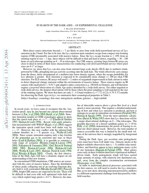
A Two-Dimensional Spectrum for Bistatic SARProcessing Using Series ReversionYew Lam Neo,Student Member,IEEE ,Frank Wong,and Ian G.Cumming,Life Senior Member,IEEEAbstract —This letter derives the two-dimensional point target spectrum for an arbitrary bistatic synthetic aperture radar con-figuration.The method described makes use of series reversion,the method of stationary phase,and Fourier transform pairs to derive the point target spectrum.The accuracy of the spectrum is controlled by keeping enough terms in the two series expansions,and is verified with a point target simulation.Index Terms —Bistatic SAR,point target spectrum,SAR simu-lation,series reversion,synthetic aperture radar (SAR).I.I NTRODUCTIONTHE IDEAL solution for bistatic synthetic aperture radar (SAR)image formation is a two-dimensional (2-D)matched filtering process.The time-domain method [1]is a direct matched filtering of the baseband signal using the exact replica of the echo signal at each location and thus gives the optimum reconstruction.However,this method is computation-ally intensive as it scales with an order of O ((N ×M )2),where N ×M is the number of pixels in the image.Efficiency can be improved by performing the focusing in the frequency domain.The point target spectrum is the basis for most efficient processing algorithms operating in the 2-D or range Doppler domain [2].The individual transmitter and re-ceiver range histories are hyperbolic,as in the monostatic case.However,because the transmit and receive range equations are not the same in the bistatic case,the total range is no longer a hyperbola.This means that the point target spectrum of the monostatic and bistatic cases are inherently different and thus,in general,monostatic algorithms are not able to focus bistatic configurations.The point target spectrum for the monostatic case has been derived in [3],and an approximate point target spectrum for some bistatic cases has been derived in [4].In [5],it was shown how the 2-D spectrum can be modified to change the leader–follower bistatic case with a constant baseline into an equivalent monostatic case for which a conventional monostatic algorithm can be applied.In this letter,the 2-D frequency spectrum is derived for the general bistatic case,based on the reversion of a series approximation.A simulation is performed to illustrate its accuracy.Manuscript received June 1,2006;revised July 10,2006.Y .L.Neo is with the DSO National Laboratories,Singapore 118230.F.Wong is with MacDonald,Dettwiler and Associates Ltd.,Richmond,BC V6V 2J3,Canada.I.G.Cumming is with the Department of Electrical and Computer Engineer-ing,University of British Columbia,Vancouver,BC V6T 1Z4,Canada.Digital Object Identifier 10.1109/LGRS.2006.885862Fig.1.General bistatic configuration of transmitter and receiver at η=0.The results of this letter will be useful for developing efficient bistatic algorithms operating in the 2-D frequency domain or the range Doppler domain.Several bistatic airborne experi-ments involving geometries with fixed baseline [6]and [7]were conducted recently.For these flight configurations,point targets with the same closest range of approach would have the same range Doppler histories.Thus,using the same point target spectrum,we are able to focus a family of points and hence achieve processing efficiency.In another paper [8],this method was used to develop an efficient frequency-domain matched filter.II.B ISTATIC SAR S IGNAL M ODELA general bistatic SAR geometry is shown in Fig.1,includ-ing nonparallel tracks,unequal velocities,and antenna squint.The time-domain matched filter is constructed by forming the instantaneous slant range to a point target,referred to as the range equationR (η)=R T (η)+R R (η)=V 2T η2+R 2Tcen −2V T ηR Tcen sin θsqT +V 2R η2+R 2Rcen −2V R ηR Rcen sin θsqR(1)where ηis azimuth time,V is the velocity of the platform,R is the instantaneous range to the point target,and the subscripts T and R refer to the transmitter and receiver,respectively.The subscript,cen,refers to a target at the center of the imaged area.Zero azimuth time (η=0)is defined as the midpoint of the integration path for the transmitter,as shown in Fig.1.The receiver position is shown at the same time.θsqT is the squint1545-598X/$25.00©2007IEEEangle of the transmitter,andθsqR is the squint angle of the receiver at this time.After demodulation to baseband,the received signal can be written in terms of the range time(fast time)τand azimuth time (slow time)ηs(τ,η)=ρrτ−R(η)cw az(η)exp−j2πR(η)λ(2)whereρr(·)is the range envelope and the azimuth envelope w az(·)is determined by the composite antenna pattern.III.D ERIVATION OF THE S IGNAL S PECTRUMTo derive the2-D spectrum,thefirst step is to remove the linear phase and the linear range cell migration(LRCM).This reason for this step will become apparent when we apply the series reversion at a later step.After removal of these terms,the point target signal in the time domain iss A(τ,η)=ρrτ−R1(η)cw az(η)exp−j2πR1(η)λ(3)whereR1(η)=R cen+k2η2+k3η3+k4η4+ (4)is the range after removing the linear term and R cen is the sum of R Tcen and R Rcen,and the coefficientsk2=12!dR2T(η)dη2+dR2R(η)dη2η=0(5)k3=13!dR3T(η)dη3+dR3R(η)dη3η=0(6)k4=14!dR4T(η)dη4+dR4R(η)dη4η=0(7)...are evaluated at the aperture center.The derivatives of the transmitter range are given byd2R T(η)dη2η=0=V2Tcos2θsqTR Tcen(8)d3R T(η)dη3η=0=3V3T cos2θsqT sinθsqTR2Tcen(9)d4R T(η)dη4η=0=3V4T cos2θsqT(4sin2θsqT−cos2θsqT)R3Tcen.(10)Similar equations can be written for the derivatives of the receiver range R R(η).If we keep the terms up to the fourth-order term in(8)and expand up to the fourth azimuth frequency term,the2-D point target spectrum is given byS A(fτ,η)=W r(fτ)w az(η)exp−j2π(f o+fτ)R1(η)c(11)where W r(·)represents the spectral shape(e.g.,bandwidth)of the transmitted pulse,f o corresponds to the center frequency,and fτis the range frequency.Next,we perform an azimuth Fourier transform(FT).Using the method of stationary phase [9],azimuth frequency is related to azimuth time by−cf o+fτfη=2k2η+3k3η2+4k4η3+ (12)where fηis the azimuth frequency.We can derive an expression ofηin terms of fηby using the series reversion(refer to the Appendix).In the forward function(26),we replace x byη,y by(−c/(f o+fτ))fη,and substitute the coefficients of x by the coefficients ofη.Inverting this power series,we arrive atη(fη)=A1−cf o+fτfη+A2−cf o+fτfη2+A3−cf o+fτfη3+ (13)The rationale for removal of the linear phase term and LRCM becomes clear at this step.In order to apply the series reversion directly in(12),we should remove the constant term in the forward function since the constant term is absent in the forward function(26).Both the linear phase term and the LRCM term are removed so that there is no constant term left after applying azimuth FT to(11).1Using(13)with(11),we obtain the2-D spectrum of s A(τ,η) S A(fτ,fη)=W r(fτ)W az(fη)exp−j2πfηη(fη)×exp−j2π(f o+fτ)cR1(η(fη))(14)where W az(·)represents the shape of the Doppler spectrum and is approximately a scaled version of the azimuth time envelope w az(·).To get the2-D point target spectrum for s(τ,η),we reintroduce the LRCM and linear phase into s A(τ,η)in(3)s(τ,η)=s Aτ−k1ηc,ηexp−j2πf o k1cη=ρrτ−R1(η)+k1ηcw az(η)×exp−j2πf o R1(η)c+f o k1ηc(15) wherek1=dR T(η)dηη=0+dR R(η)dηη=0.(16) The derivatives(16)at the aperture center are given bydR T(η)dηη=0=−V T sinθsqT(17)dR R(η)dηη=0=−V R sinθsqR.(18)1An alternate approach is to move the constant term to the left-hand side of (12)and treat the whole term on the left-hand side as y.We would still end up with the same solution(20).NEO et al.:TWO-DIMENSIONAL SPECTRUM FOR BISTATIC SAR PROCESSING95 TABLE IS IMULATION P ARAMETERSc.(20)The accuracy of the spectrum is limited by the number of terms used in the expansion of(20).In general,we would like to limit the uncompensated phase error to be within±π/4,in order to avoid significant deterioration of the image quality.IV.S IMULATION R ESULTSTo prove the validity of the formulation,a point target signal is simulated in the time domain and matchedfiltering is carried out in the2-D frequency domain.Processing efficiency is achieved by focusing point targets in an invariance region with the same matchedfilter.The size of the invariance region is dependent upon the radar parameters and the imaging geometry. The purpose of this letter is to prove accuracy of the derived spectrum.Analysis of the extent of the invariance region will be investigated in a separate paper.The simulation uses airborne SAR parameters given in Table I.An appreciable amount of antenna squint is assumed, as well as unequal platform velocities and nonparallel tracks. The axes are defined in a right-hand Cartesian coordinate system with theflight direction of the transmitter parallel to the y direction and z is the altitude of the aircraft.The oversampling ratio is1.33in range and azimuth.Rectangular weighting is used for both azimuth and range processing.If we keep the terms up to a fourth-order term in(20)and expand up to the fourth azimuth frequency term,the2-D point target spectrum is given byS(fτ,fη)=W r(fτ)W azfη+(f o+fτ)k1cexp{jφ(fτ,fη)}(21) where the phase is given byφ(fτ,fη)=−2πf o+fτcR cen+2πc4k2(f o+fτ)fη+(f o+fτ)k1c2+2πc2k38k32(f o+fτ)2fη+(f o+fτ)k1c3+2πc39k23−4k2k464k52(f o+fτ)3fη+(f o+fτ)k1c4.(22) The magnitudes of the cubic and quartic terms in(22)are∆φ3≈2πc2k38k32f2oB a23(23)∆φ4≈2πc39k23−4k2k464k52f3oB a24(24)where B a is the Doppler bandwidth.For this simulation case,B a=150Hz,k2=1.31m/s,k3=0.0146m/s2,and k4=0.000184m/s3.The phase component∆φ3is more thanπ/4 and∆φ4is much less thanπ/4.Therefore,it is sufficient to only terms up to the cubic term in the phase expansion (22)for accurate focusing in this radar case.Matchedfiltering is performed by multiplying the2-D spectrum of the point target by exp(−jφ(fτ,fη)).The point target spectrum after matchedfiltering has a 2-D envelope given by W r and W az in(21),as shown in Fig.2(a).Note that the spectrum has a skew as a result of the range/azimuth coupling.This results in skewed sidelobes as shown in Fig.2(b).However,in order to measure image quality parameters such as the3-dB impulse response width(IRW)and the peak sidelobe ratio(PSLR),it is convenient to remove the skew by shearing the image along the range time axis by the amountδτ=−V T sin(θT)+V R sin(θR)cη.(25)The deskewed sidelobes are seen in Fig.2(d).The deskewing operation is equivalent to deskewing the spectrum,as shown in Fig.2(c).The quality of the focus can be examined using the one-dimensional expansions shown in Fig.3.The excellent focus is demonstrated by the IRW,which meets the theoretical limits96IEEE GEOSCIENCE AND REMOTE SENSING LETTERS,VOL.4,NO.1,JANUARY2007Fig.2.Point target spectrum and image before and after the shear operation.(a)Spectrum after matched filtering.(b)Point target after matched filtering.(c)Spectrum after shear operation.(d)Point target after shearoperation.Fig.3.Measurement of point target focus using a matched filter derived fromthe new 2-D point target spectrum.in range (1.184/1.33=0.89)and in azimuth (1.188/1.33=0.89)for rectangular weighting.Furthermore,the sidelobes agree with the theoretical values of −10and −13.3dB for the integrated sidelobe ratio (ISLR)and PSLR,respectively.In addition,the symmetry of the sidelobes is another indication of correct matched filter phase.V .C ONCLUSIONThe 2-D point target spectrum for the general bistatic case is developed by expressing the bistatic range equation as a power series and using the method of series reversion to express azimuth time as a function of azimuth frequency during the azimuth FT.This results in a power series expression for the spectrum of the point target,whose accuracy is controlled by the degree of the power series.The accuracy of the derived spectrum is confirmed using a simulation where the point target is simulated in the time domain,then compressed using a 2-D matched filter derived from the spectrum.The method of series reversion is also applicable to mono-static stripmap and spotlight situations where the simple hyper-bolic range equation does not hold.A PPENDIXS ERIES R EVERSIONSeries reversion is the computation of the coefficients of the inverse function given those of the forward function (26).For a function expressed in a series with no constant term a 0=0y =a 1x +a 2x 2+a 3x 3+···(26)the series expansion of the inverse function is given byx =A 1y +A 2y 2+A 3y 3+···.(27)Substituting (27)into (26),the following equation is obtained:y =a 1A 1y +a 2A 21+a 1A 2 y 2+a 3A 31+2a 1A 1A 2+a 1A 3 y 3+···.(28)By equating terms,the coefficients of the inverse function areA 1=a −11A 2=−a −31a 2A 3=a −512a 22−a 1a 3 (29)The formula for the n th coefficient is given in [10],as summa-rized in the handbook [11].A CKNOWLEDGMENTThe authors would like to thank DSO National Laboratories,Singapore,for providing scholarship funding for Y .L.Neo.R EFERENCES[1]B.Barber,“Theory of digital imaging from orbital synthetic apertureradar,”Int.J.Remote Sens.,vol.6,no.6,pp.1009–1057,1985.[2]I.G.Cumming and F.H.Wong,Digital Processing of Synthetic ApertureRadar Data:Algorithms and Imp lementation .Norwood,MA:Artech House,2005.[3]R.K.Raney,“A new and fundamental Fourier transform pair,”inProc.Int.Geosci.Remote Sens.Symp.,Clear Lake,TX,May 1992,pp.106–107.[4]O.Loffeld,H.Nies,V .Peters,and S.Knedlik,“Models and useful re-lations for bistatic SAR processing,”IEEE Trans.Geosci.Remote Sens.,vol.42,no.10,pp.2031–2038,Oct.2004.[5]D.D’Aria,M.Guarnieri,and F.Rocca,“Focusing bistatic synthetic aper-ture radar using dip move out,”IEEE Trans.Geosci.Remote Sens.,vol.42,no.7,pp.1362–1376,Jul.2004.[6]P.Dubois-Fernandez,H.Cantalloube,B.Vaizan,G.Krieger,R.Horn,M.Wendler,and V .Giroux,“ONERA-DLR bistatic SAR campaign:Plan-ning,data acquistion,and first analysis of bistatic scattering behaviour of natural and urban targets,”Proc.Inst.Electr.Eng.—Radar,Sonar Navig.,vol.153,no.3,pp.214–223,Jun.2006.[7]I.Walterscheid,A.Brenner,and J.Ender,“Geometry and system aspectsfor a bistatic airborne SAR-experiment,”in Proc.EUSAR ,Ulm,Germany,May 2004,pp.567–570.[8]Y .Neo,F.Wong,and I.G.Cumming,“An efficient non-linear chirp scal-ing method of focusing bistatic SAR images,”in Proc.EUSAR ,Dresden,Germany,May 2006.[CD-ROM].[9]A.Papoulis,Signal Analysis .New York:McGraw-Hill,1977.[10]P.M.Morse and H.Feshbach,Methods of Theoretical Physics ,1st ed.New York:McGraw-Hill,1953.[11]H.B.Dwight,Table of Integrals and Other Mathematical Data ,4th ed.New York:Macmillan,1961.。
Q4X传感器快速入门指南说明书
Quick Start GuideClass 1 laser CMOS sensor with a discrete (PNP or NPN) output. Patent pending.This guide is designed to help you set up and install the Q4X Sensor. For complete information on programming, performance, troubleshooting,dimensions, and accessories, please refer to the Instruction Manual at . Search for p/n 181483 to view the Instruction Manual. Use of this document assumes familiarity with pertinent industry standards and practices.For illustration purposes, the threaded barrel model Q4X images are used throughout this document.WARNING:•Do not use this device for personnel protection•Using this device for personnel protection could result in serious injury or death.•This device does not include the self-checking redundant circuitry necessary to allow its use in personnel safetyapplications. A device failure or malfunction can cause either an energized (on) or de-energized (off) output condition.FeaturesFigure 1. Sensor Features—Threaded Barrel Models1.Output Indicator (Amber)2.Display3.ButtonsFigure 2. Sensor Features—Flush Mount Models2The display is a 4-digit, 7-segment LED. The main screen is the Run Mode screen, which shows the percentage matched to the taught reference surface. A display value of 999P indicates the sensor has not been taught.1.Stability Indicator (STB = Green)2.Active TEACH Indicators•COD = Intensity and distance windows for clear object detection•••Stability Indicator (STB)•On—Stable signal within the specified sensing range•Flashing—Marginal signal, the target is outside the limits of thespecified sensing range, or a multiple peak condition exists •Off—No target detected within the specified sensing rangeButtonsUse the sensor buttons (SELECT)(TEACH), (+)(LO/DO), and (-)(MODE) to program the sensor.Figure 4. Buttons(SELECT)(TEACH)•Press to select menu items in Setup mode•Press and hold for longer than 2 seconds to start the ClearObject Detection TEACH mode(+)(LO/DO)•Press to navigate the sensor menu in Setup mode•Press to change setting values; press and hold to increasenumeric values•Press and hold for longer than 2 seconds to switch between lightoperate (LO) and dark operate (DO)Q4X Stainless Steel Laser Sensor for Clear Object DetectionOriginal Document 187731 Rev. D11 January 2023187731(-)(MODE)•Press to navigate the sensor menu in Setup mode•Press to change setting values; press and hold to decreasenumeric values•Press and hold for longer than 2 seconds to enter Setup modeNote: When navigating the menu, the menu items loop.Laser Description and Safety InformationCAUTION:•Return defective units to the manufacturer.•Use of controls or adjustments or performance of procedures other than those specified herein may result inhazardous radiation exposure.•Do not attempt to disassemble this sensor for repair. A defective unit must be returned to the manufacturer.≤ 510 mm Models - IEC 60825-1:2007 Class 1 LaserClass 1 lasers are lasers that are safe under reasonably foreseeable conditions of operation, including the use of optical instruments for intrabeamviewing.Laser wavelength: 655 nm Output: < 0.20 mW Pulse Duration: 7 µs to 2 ms> 510 mm Models - IEC 60825-1:2014 Class 1 LaserClass 1 lasers are lasers that are safe under reasonably foreseeable conditions of operation, including the use of optical instruments for intrabeam viewing.Laser wavelength: 655 nm Output: < 0.39 mW Pulse Duration: 7 µs to 2 msInstallationInstall the Safety LabelThe safety label must be installed on Q4X sensors that are used in the United States.Note: Position the label on the cable in a location that has minimal chemical exposure.1.Remove the protective cover from the adhesive on the label.2.Wrap the label around the Q4X cable, as shown.3.Press the two halves of the label together.Figure 5. Safety Label InstallationSensor Orientation and Mounting Considerations for Transparent and Clear Object DetectionOptimize the reliable detection of transparent and clear objects by applying these principals when selecting your reference surface, positioning your sensor relative to the reference surface, and presenting your target. The robust detection capabilities of the Q4X will allow successful detection even under non-ideal conditions in many cases.1.Select a reference surface with these characteristics where possible:•Matte or diffuse surface finish •Fixed surface with no vibration•Dry surface with no build-up of oil, water, or dust2.Position the reference surface between 50 and 300 mm (threaded barrel models) or 60 mm and 310 mm (flush mount models).3.Position the target to be detected as close to the sensor as possible, and as far away from the reference surface as possible.4.Angle the sensing beam relative to the target and relative to the reference surface 10 degrees or more. - Tel: + 1 888 373 6767P/N 187731 Rev. DFigure 6. Mounting considerationsFigure 7. Common problems and solutions for detecting clear objectsThe object is close to the reference surfacePROBLEM:Move the target closer to the sensorSOLUTION:PROBLEM:Move the sensor closer to the targetSOLUTION:Mount the Device1.If a bracket is needed, mount the device onto the bracket.2.Mount the device (or the device and the bracket) to the machine or equipment at the desired location. Do not tighten the mounting screws atthis time.3.Check the device alignment.4.Tighten the mounting screws to secure the device (or the device and the bracket) in the aligned position.P/N 187731 Rev. D - Tel: + 1 888 373 67673Wiring Diagram —Threaded Barrel Models+–Note: Open lead wires must be connected to a terminal block.Key1 = Brown2 = White3 = Blue4 = Black5 = GrayNote: The input wire function is user-selectable; see the Instruction Manual for details. The default for the input wire function is off (disabled).Wiring Diagram—Flush Mount ModelsNPN ModelsPNP ModelsKey1 = Brown2 = White3 = Blue4 = BlackNote: Open lead wires must be connected to a terminal block.Note: The input wire function is user-selectable; see the Instruction Manual for details. The default for the input wire function is off (disabled).Cleaning and MaintenanceClean the sensor when soiled and use with care.Handle the sensor with care during installation and operation. Sensor windows soiled by fingerprints, dust, water, oil, etc. may create stray light that may degrade the peak performance of the sensor. Blow the window clear using filtered, compressed air, then clean as necessary using only water and a lint-free cloth.Sensor ProgrammingProgram the sensor using the buttons on the sensor or the remote input (limited programming options).In addition to programming the sensor, use the remote input to disable the buttons for security, preventing unauthorized or accidental programming changes. See the Instruction Manual, p/n 181483 for more information.Setup ModeAccess Setup mode and the sensor menu from Run mode by pressing and holding MODEthrough the menu. Press SELECT SELECT to select a submenu option and return to the top menu, or press and hold and return immediately to Run mode.To exit Setup mode and return to Run mode, navigate toand press SELECT . - Tel: + 1 888 373 6767P/N 187731 Rev. DFigure 8. Sensor Menu Map—Channel 1LO = On pulse when a target is detected inside of the switch point(s)DO = On pulse when a target is detected outside of the switch point(s)sec range, set Delay Timer value (seconds have decimal)( default setting)when is selected,1 to 9 ms is range available when Response Speed is Basic TEACH InstructionsUse the following instructions to teach the Q4X sensor.1.Align the sensor to a stable reference surface.2.Rigidly mount the sensor in this alignment.3.Press and hold TEACH for longer than 2 seconds to start the TEACH mode.4.Press TEACH to teach the reference surface. The reference surface is taught, the currently selected switch point value is displayed, and the sensor returns to run mode.The Q4X sensor records the distance to the reference surface and the amount of laser light returned by the reference surface. The output is switched when an object passing between the sensor and the reference surface changes the perceived distance or amount of returned light. The Q4X is able to detect the very small changes caused by transparent and clear objects. Typical reference surfaces are metal machine frame, conveyor side rail, or mounted plastic targets. Please contact Banner Engineering if you require assistance setting up a stable reference surface in your application.The Q4X sensor can be taught non-ideal reference surfaces, such as surfaces outside of the sensor range or very dark surfaces. Teaching non-ideal reference surfaces may enable applications other than transparent or clear object detection, but best results for transparent or clear object detection require a stable reference surface as described above in Sensor Orientation and Mounting Considerations for Transparent and Clear Object Detection on page 2.Manual Adjustments1.flashes slowly.P/N 187731 Rev. D - Tel: + 1 888 373 676752.After the TEACH process is completed, the taught reference point, a combination of the measured distance and returned signal intensity from theThe display shows the current match percentage relative to the taught reference point. The switch point defines the sensitivity; the output switches when the current match percentage crosses the switch point.Your specific application may require some adjustment of the switch point, but these values are recommended starting switch points for common applications.Light Operate/Dark OperateThe default output configuration is light operate. To switch between light operate and dark operate, use the following instructions:1.Press and hold LO/DO for longer than 2 seconds. The current selection displays.2.Press LO/DO again. The new selection flashes slowly.3.Press SELECT to change the output configuration and return to Run mode.Note: If neither SELECT nor LO/DO are pressed after step 2, the new selection flashes slowly for a few seconds, then flashes quickly and the sensor automatically changes the output configuration and returns to Run mode.Locking and Unlocking the Sensor ButtonsUse the lock and unlock feature to prevent unauthorized or accidental programming changes.Three settings are available:•—The sensor is unlocked and all settings can be modified (default).•— The sensor is locked and no changes can be made.•—The switch point value can be changed by teaching or manual adjustment, but no sensor settings can be changed through the menu.When in mode,displays when the (SELECT)(TEACH) button is pressed. The switch point displays when (+)(LO/DO) or (-)(MODE)are pressed, butdisplays if the buttons are pressed and held.When inmode, displays when (+)(LO/DO) or (-)(MODE) are pressed and held. To access the manual adjust options, briefly press and release (+)(LO/DO) or (-)(MODE). To enter TEACH mode, press the (SELECT)(TEACH) button and hold for longer than 2 seconds.To enter.SpecificationsSensing BeamVisible red Class 1 laser, 655 nm Supply Voltage (Vcc)10 V DC to 30 V DCPower and Current Consumption, exclusive of load < 675 mW Sensing Range25 mm to 300 mm (0.98 in to 11.81 in)Output ConfigurationBipolar (1 PNP and 1 NPN) output Output Rating100 mA total maximum (protected against continuous overload and short circuit)Off-state leakage current: < 5 µA at 30 V DCPNP On-state saturation voltage: < 1.5 V DC at 100 mA load NPN On-state saturation voltage: < 1.0 V DC at 100 mA load Remote InputAllowable Input Voltage Range: 0 to VccActive Low (internal weak pullup—sinking current): Low State < 2.0 V at 1 mA max.Supply Protection CircuitryProtected against reverse polarity and transient overvoltagesResponse Speed User selectable:•—1.5 milliseconds •—3 milliseconds •—10 milliseconds •—25 milliseconds•—50 millisecondsChemical CompatibilityCompatible with commonly used acidic or caustic cleaning and disinfecting chemicals used in equipment cleaning and sanitation. ECOLAB ® certified.Compatible with typical cutting fluids and lubricating fluids used in machining centers Application NoteFor optimum performance, allow 10 minutes for the sensor to warm up - Tel: + 1 888 373 6767P/N 187731 Rev. DDelay at Power Up < 750 msMaximum TorqueSide mounting: 1 N·m (9 in·lbs)Nose mounting: 20 N·m (177 in·lbs)Ambient Light Immunity > 5,000 lux at 300 mm ConnectorIntegral 5-pin M12 male quick-disconnect connector ConstructionHousing: 316 L stainless steel Lens cover: PMMA acrylicLightpipe and display window: polysulfoneEnvironmental Rating IP67 per IEC60529IP68 per IEC60529IP69K per DIN 40050-9IP rating is dependent on proper cordset installation.VibrationMIL-STD-202G, Method 201A (Vibration: 10 Hz to 60 Hz, 0.06 inch (1.52 mm) double amplitude, 2 hours each along X, Y and Z axes), with device operating ShockMIL-STD-202G, Method 213B, Condition I (100G 6x along X, Y, and Z axes, 18shocks), with device operating Operating Conditions–10 °C to +50 °C (+14 °F to +122 °F)35% to 95% relative humidity Storage Temperature–25 °C to +75 °C (–13 °F to +167 °F)Excess Gain—Threaded Barrel ModelsTable 1:Excess Gain (Excess Gain 1)Excess Gain—Flush Mount ModelsTable 2:Excess Gain (Excess Gain 2)Beam Spot SizeTable 3: Beam Spot Size—300 mm ModelsRequired Overcurrent ProtectionWARNING: Electrical connections must be made by qualified personnel in accordance with local and national electrical codes and regulations.Overcurrent protection is required to be provided by end product application per the supplied table.Overcurrent protection may be provided with external fusing or via Current Limiting, Class 2 Power Supply.Supply wiring leads < 24 AWG shall not be spliced.For additional product support, go to .• excess gain provides increased noise immunity• excess gain available in 10 ms, 25 ms, and 50 ms response speeds only •excess gain provides increased noise immunityP/N 187731 Rev. D - Tel: + 1 888 373 67677CertificationsBanner Engineering BV Park Lane, Culliganlaan 2F bus3, 1831 Diegem, BELGIUMTurck Banner LTD Blenheim House, Blenheim Court,Wickford, Essex SS11 8YT, Great BritainIndustrial Control Equipment 3TJJ Class 2 powerUL Environmental Rating: Type 1chemical compatibility certifiedECOLAB is a registered trademark of Ecolab USA Inc. All rights reserved.FCC Part 15 Class AThis equipment has been tested and found to comply with the limits for a Class A digital device, pursuant to part 15 of the FCC Rules. These limits are designed to provide reasonable protection against harmful interference when the equipment is operated in a commercial environment. This equipment generates, uses, and can radiate radio frequency energy and, if not installed and used in accordance with the instruction manual, may cause harmful interference to radio communications. Operation of this equipment in a residential area is likely to cause harmful interference in which case the user will be required to correct the interference at his own expense.Industry CanadaThis device complies with CAN ICES-3 (A)/NMB-3(A). Operation is subject to the following two conditions: 1) This device may not cause harmful interference; and 2) This device must accept any interference received, including interference that may cause undesired operation.Cet appareil est conforme à la norme NMB-3(A). Le fonctionnement est soumis aux deux conditions suivantes : (1) ce dispositif ne peut pas occasionner d'interférences, et (2) il doit tolérer toute interférence, y compris celles susceptibles de provoquer un fonctionnement non souhaité du dispositif.Banner Engineering Corp. Limited WarrantyBanner Engineering Corp. warrants its products to be free from defects in material and workmanship for one year following the date of shipment. Banner Engineering Corp. will repair or replace, free of charge, any product of its manufacture which, at the time it is returned to the factory, is found to have been defective during the warranty period. This warranty does not cover damage or liability for misuse, abuse, or the improper application or installation of the Banner product.THIS LIMITED WARRANTY IS EXCLUSIVE AND IN LIEU OF ALL OTHER WARRANTIES WHETHER EXPRESS OR IMPLIED (INCLUDING, WITHOUT LIMITATION, ANY WARRANTY OF MERCHANTABILITY OR FITNESS FOR A PARTICULAR PURPOSE), AND WHETHER ARISING UNDER COURSE OF PERFORMANCE, COURSE OF DEALING OR TRADE USAGE.This Warranty is exclusive and limited to repair or, at the discretion of Banner Engineering Corp., replacement. IN NO EVENT SHALL BANNER ENGINEERING CORP. BE LIABLE TO BUYER OR ANY OTHER PERSON OR ENTITY FOR ANY EXTRA COSTS, EXPENSES, LOSSES, LOSS OF PROFITS, OR ANY INCIDENTAL, CONSEQUENTIAL OR SPECIAL DAMAGES RESULTING FROM ANY PRODUCT DEFECT OR FROM THE USE OR INABILITY TO USE THE PRODUCT, WHETHER ARISING IN CONTRACT OR WARRANTY, STATUTE, TORT, STRICT LIABILITY, NEGLIGENCE, OR OTHERWISE.Banner Engineering Corp. reserves the right to change, modify or improve the design of the product without assuming any obligations or liabilities relating to any product previously manufactured by Banner Engineering Corp. Any misuse, abuse, or improper application or installation of this product or use of the product for personal protection applications when the product is identified as not intended for such purposes will void the product warranty. Any modifications to this product without prior express approval by Banner Engineering Corp will void the product warranties. All specifications published in this document are subject to change; Banner reserves the right to modify product specifications or update documentation at any time. Specifications and product information in English supersede that which is provided in any other language. For the most recent version of any documentation, refer to: .For patent information, see /patents.© Banner Engineering Corp. All rights reserved。
Part one Remote Sensing(lesson thirteen)
However, rarely is digital processing and analysis carried out as a complete replacement for manual interpretation. Often, it is done to supplement and assist the human analyst.
mottled杂色的;斑驳的;斑点的 canopy (篷形)遮盖物; profile侧面(像),侧影 eliminate排除,消除,消灭 Landform 地形 marina小艇码头 recreational消遣的;娱乐的;休养的
In order to take advantage of and make good use of remote sensing data, we must be able to extract meaningful information from the imagery. This brings us to the topic of discussion in this chapter interpretation and analysis - the sixth element of the remote sensing process which we defined in Chapter 1.
Stereoscopically ad. 实(立)体镜地 Simulate 模仿,模拟; benefit对...有益,有益于 visualization 可视化 recognition认出,识别;认识 dramatically戏剧性地;引人注目地 tone 色调 pattern图案mputer environment is more amenable to handling complex images of several or many channels or from several dates. In this sense, digital analysis is useful for simultaneous analysis of many spectral bands and can process large data sets much faster than a human interpreter.
机载平行等速双基SAR极坐标格式成像算法
机载平行等速双基SAR的极坐标格式成像算法摘要:平行等速双基sar是指收发平台速度大小和方向均相同的双基sar系统,该构型具有广阔的应用前景。
在此将传统适用于单基地sar成像的极坐标格式算法(pfa)加以改进,使之适用于平行等速双基sar成像处理。
由于收发异置,回波信号在接收平面和发射平面的斜距几何关系比较复杂。
为了便于后续的二维插值操作,用一个新的几何模型来描述收发平面上斜距的关系。
该算法具有传统pfa算法的操作简单,易于实现的特点。
最后通过仿真数据的成像处理对该方法进行了验证。
关键词:双基合成孔径雷达;极坐标格式算法;成像算法;几何模型引言双基sar在地物分类和识别、干涉测高、高分辨宽域成像等方面有着广阔的应用前景。
与单基地sar相比,双基地sar的主要优点有:作用距离更远,获取信息更丰富,机动性和隐蔽性更高,抗干扰和抗截获性能更好。
关于双基sar系统的研究,在文献[13]中都有所讨论。
在各种构型的双基sar中,接收机和发射机平台速度大小相同,方向平行的双基sar(平行等速双基sar)具有方位不变性,适合大面积连续成像,许多文献讨论过这种构型的双基sar 成像方法。
时域逐点匹配方法可以用于任意一类的双基sar,该方法是理论上最优的,但缺点是运算量效率很低,文献[4]对该方法进行了研究;loffeld用傅里叶变换将回波数据从慢时间域变到多普勒域时,把收、发斜距分别在各自的驻相点处做二阶泰勒近似,然后对二阶近似式用驻相点法求出其多普勒域表达式[5]。
此算法可以得到任意构型下双基二维频域表达式,但其主要缺点是其精度不高,对精确成像不利。
基于这个频谱,文献[68]提出了改进的双基sar成像算法。
neo把回波的相位历程在慢时间进行高阶泰勒级数展开,然后通过使用级数反演法求出信号二维频域的近似表达式[9]。
在该方法的基础上,wong和neo分别提出了改进的非线性csa算法[10]和改进的距离多普勒算法[11]。
DIP开关用户手册说明书
Safety Precautions■CautionsUse the DIP Switch within the rated voltage and current ranges, otherwise the DIP Switch may have a shortened life expectancy, radiate heat, or burn out. This particularly applies to the instanta-neous voltages and currents when switching.■Correct UseCircuit DesignAlthough the minimum current is 10 µA (3.5 VDC), contact reli-ability may need to be improved in some cases. This is particu-larly true when switching causes an increase in instantaneous current, such as in C-MOS IC applications. Do not let the peak current exceed the rated value here or any other time.Only BCD/hexadecimal 1-2-4-8 code is available for A6C/A6CV/ A6R/A6RV models. If BCD/hexadecimal 1-2-4-8 complement code is required, make the appropriate provisions in the circuit. MountingNormally the default striker setting is OFF for slide-type DIP Switches and the default rotor setting is 0 for Rotary DIP Switches. Do not change these settings when mounting, solder-ing, washing or drying Switches. In rare cases, the striker may be deformed by heat generated during soldering.1.Automatic Insertion MachineUse a body stopper system for the chute stopper of automatic insertion machines. When mounting Switches using an insertion machine incorporating a half-lead stopper, make sure the machine will not deform the terminals of the Switch, or improper insertion may result. Check actual mounting conditions prior to using a half-lead stopper system.A printed circuit board that is 1.2 to 1.6 mm thick is recom-mended.Holes on the PCB should be at least 0.9 mm in diameter for auto-matic insertion.2.Manual or IC Socket InsertionCommercially available insertion tools are recommended for mounting ICs on PCBs.T erminal pitch, dimensions and other features are identical to that of standard ICs for IC socket compatibility (except for the A6S-H and A6H).Align the terminals so they slide in simultaneously when the Switch is inserted into socket holes or into mounting holes pre-drilled at the specified dimensions. Apply downward force on the Switch until the terminals are properly seated on the PCB.Do not try to remove a Switch by inserting a screwdriver between it and the PCB, and then twisting the screwdriver to peel the Switch off. Use a commercially available inserter/remover to remove the Switch.SolderingObserve the following conditions when soldering the DIP Switch.1.General Precautions for SolderingMake sure that the striker of slide-type DIP Switches is set fully to either ON or OFF. (For A6E and A6ER models, however, set the Switch to OFF before soldering.) Make sure that Rotary DIP Switches are correctly set to 0. Misalignment may result in reduced sensitivity due to the soldering heat.Before soldering the Switch on a PCB, make sure there is no unnecessary space between the Switch and the PCB.Before soldering the Switch on a multilayer PCB, conduct a test to make sure the Switch will not be deformed by soldering heat on the pattern or land of the multilayer PCB.2.Automatic Soldering Bath (Except A6S-H/A6H)Soldering temperature: 260°C max.Soldering time: 5 s max. for a 1.6-mm thick, single-side PCBDo not use an automatic soldering bath or manual soldering for A6S-H or A6H models.Confirm in advance that flux will not bubble up onto the side of the PCB to which the Switch is mounted. Depending on the type of Switch, the flux may have an adverse effect if it enters the Switch. The A6S-H and A6H are designed specifically for reflow solder-ing. Do not use an automatic soldering bath or manual solderingfor these models.3.Reflow SolderingObserve the following conditions for reflow soldering the A6S-HDo not use reflow soldering for any models other than the A6S-H and A6H. Otherwise the plastic case may melt or deform.The soldering conditions and the temperature around the Switch may vary with the type of reflow bath. Check the temperature pro-file and confirm soldering conditions as well as the amount of heat applied to the Switch prior to soldering.4.Manual Soldering (Except A6S-H/A6H)Soldering temperature: 350°C at the tip of the soldering iron. Soldering time: 3 s max. for a 1.6-mm thick, single-side PCBDo not solder the Switch more than twice including any rectifica-tion soldering. An interval of five minutes is required between the first and second soldering.ing FluxMaking mistakes in the type of flux or in the amount or method in which it is applied can cause flux to enter the interior of the Switch, with adverse effects on Switch performance. Assess the proper flux, conditions, and methods prior to using it.PCB surfaceFlux surfaceWashing1. Washable and Non-washable ModelsThe models for which washing are possible are shown in the fol-lowing table.2. Washing ProcedureUltrasonic cleaning is not available for slide-type DIP Switches with seal tape. These models may be wiped or dipped into wash-ing agents for one minute maximum.Slide-type DIP Switches with seal tape can be washed as long as the seal tape is not removed or pasted before washing. Non-com-pliance here will cause the quality of the seal to decline.Washing equipment incorporating more than one washing bath can be used to clean washable models, provided that the wash-able models are cleaned for one minute maximum per bath and the total cleaning time does not exceed three minutes.3. Washing AgentsApply alcohol-based solvents to clean washable models. Do not apply water or any other agents to clean any washable models,as such agents may degrade the materials or performance of the Switch.4. Washing PrecautionsDo not impose any external force on washable models while washing.Do not clean washable models immediately after soldering. The cleaning agent may be absorbed into the incomplete seal through respiration as the Switch cools. Wait for at least three minutes after soldering before cleaning.Do not use washable Switches submerged in water or in locations exposed to water.Handling1. Slide-type DIP Switch operationDo not apply excessive operating force to the Switch. Otherwise the Switch may be damaged or deformed, and the switch mecha-nism may malfunction as a result. Apply an operating force not exceeding 9.8 N. (Operate the actuator one operation at a time.Do not operate the Switch from the top of actuator. Otherwise the actuator may be damaged, so operate the Switch from the lower part of the actuator.) Apply the operating load from the side of the striker. Do not apply a load from an angle or from above the Set slide-type DIP Switches with a tiny, rounded object, such as the tip of a ball-point pen or a small screwdriver. Do not set the DIP Switch using tweezers or any other sharp object that may damage it. Do not set the DIP Switch using the point of a mechan-ical pencil, or lead powder or fragments may fall into the Switch and internal circuit board, causing the DIP Switch to malfunction and reducing the dielectric strength of the circuit board.Although raised-type and piano-type strikers can be operated by fingertip, do not push too hard or too fast because this will deform or damage the striker.When setting or operating the A6H, use narrow-headed tweezers or similar implement (without a sharp end), to enable smooth,horizontal operation. Pushing the striker at an angle, or applying excessive load from above may damage or deform the striker and thereby prevent operation.2. Rotary DIP Switch OperationSet rotary-type DIP Switches with a flat-blade screwdriver that fits into the screwdriver groove. Using a screwdriver of inappropriate dimensions, or using a tool other than a flat-blade screwdriver may cause damage to the groove that may make the Switch impossible to operate.Insert the flat-blade screwdriver vertically to operate the Switch.The Switch may be damaged if the screwdriver is inserted at an angle.Do not use excessive force to operate the Switch, or it may dam-age or deform the Switch.3. SettingSet the Switch to the correct position before use. An incorrectly aligned position may result in incorrect signals.Rotary DIP Switch OperationWashable A6A, A6C, A6CV, A6D, A6DR, A6T (with seal tape), A6S-H (with seal tape), A6H (with seal tape)Non-washableA6R, A6RV, A6T (standard/raised actuator), A6S-H (standard/raised actuator), A6E, A6ER■Packing specifications•A6S-H models with embossed taping specifications are shown below.•A6H models with embossed taping specifications are shown be-low.1.5 dia. Perforations+0.4−0.2A +0.4−0.2(Seenote.)B ±0.1516±0.152±0.15P=4±0.15Tape drawing direction (ON side)T ape drawing directionLabel13 dia.13±0.5 dia.21±0.8 dia.Three, 2±0.15330±2 dia.Note:The perforations along both sides are for Switch-es with 7 poles or more. The perforations on the bottom of the diagram are not provided on Switches with 6 poles or less.Applicable models A6S-@102-PHStandard Conforms to JEITA.Package quantity 900 per reelNo. of poles 2345678910A 162424242432324444B ±0.157.511.511.511.511.514.214.220.220.2C 6.69.111.614.216.719.221.724.326.8D (22)(30)(30)(30)(30)(38)(38)(50)(50)E---------------28.428.440.440.4Applicable models A6S-@10@-PMH Standard Conforms to JEITA.Package quantity400 per reelNote:The dimensions and quantity of A6S-@104-PH/PMH and1-pole models are different. Enquire for details separately.Applicable models A6H-@102-P Standard Conforms to JEITA.Package quantity4,000 per reelNo. of poles 246810A 1212242424B ±0.13 5.55.511.511.511.5C (4.2)(6.6)(9.2)(11.7)(14.4)D(18)(18)(30)(30)(30)Applicable models A6H-@10@-PM Standard Conforms to JEITA.Package quantity500 per reelRoHS CompliantRoHS CompliantThe "RoHS Compliant" designation indicates that the listed models do not contain the six hazardous substances covered by the RoHS Directive.Reference: The following standards are used to determine compliance for the six substances.•Lead: 1,000 ppm max.•Mercury: 1,000 ppm max.•Cadmium: 100 ppm max.•Hexavelant chromium: 1,000 ppm max.•PBB: 1,000 ppm max.•PBDE: 1,000 ppm max.。
- 1、下载文档前请自行甄别文档内容的完整性,平台不提供额外的编辑、内容补充、找答案等附加服务。
- 2、"仅部分预览"的文档,不可在线预览部分如存在完整性等问题,可反馈申请退款(可完整预览的文档不适用该条件!)。
- 3、如文档侵犯您的权益,请联系客服反馈,我们会尽快为您处理(人工客服工作时间:9:00-18:30)。
A Bistatic Point Target Reference Spectrum forGeneral Bistatic SAR Processing Robert Wang,Member,IEEE,Otmar Loffeld,Senior Member,IEEE,Qurat Ul-Ann,Holger Nies,Amaya Medrano Ortiz,and Ashraf SamarahAbstract—A bistatic point target reference spectrum(BPTRS) based on Loffeld’s bistatic formula(LBF)is derived in this letter. For LBF,the same contributions of the transmitter and receiver to the total azimuth modulation are assumed.This assumption results in the failure of LBF in the extreme configuration(i.e., spaceborne/airborne configuration).For general bistatic configu-rations,the azimuth modulations are unequal for the transmitter and receiver due to the different slant ranges and velocities. Therefore,the azimuth time-bandwidth products(TBPs)from the transmitter and receiver are different;in some cases(e.g., spaceborne/airborne case),one of them might be very small,which might even result in a serious error of the principle of stationary phase.This letter uses TBP to weight the azimuth phase modula-tion contributions of the transmitter and receiver to the common azimuth spectrum to approximately obtain the point of station-ary phase of the total azimuth phase history.Simulations show that the proposed BPTRS can work well for spaceborne/airborne configurations.Index Terms—Bistatic point target reference spectrum (BPTRS),time-bandwidth product(TBP).I.I NTRODUCTIONB ISTATIC synthetic aperture radar(BSAR)is characterizedby different locations for the transmitter and receiver and hence offers considerableflexibility in designing BSAR missions[1],[2].Time-domain methods can focus BSAR data well.However, these methods always have huge computational costs.The efficiency of processing can be highly improved by performing the focusing in the frequency domain.Therefore,frequency-domain methods are preferred.The basic idea of bistatic frequency-domain processing originally comes from monosta-tic SAR data processing,which is based on the monostatic point target reference spectrum(PTRS)[3].The bistatic PTRS (BPTRS)is an important basis for processing in the2-D fre-quency domain[4],[5].However,the slant range history of BSAR includes two range histories from the transmitter and receiver,which means that the range equation consists of a double square root term.This implies that the point target refer-ence spectra of the monostatic and bistatic cases are inherently different[3],[4].Therefore,BPTRS does not offer the analyti-cal simplicity of the single square root in monostatic SAR.Manuscript received September27,2007;revised November22,2007and April1,2008.This work was supported by the Germany Science Foundation under Grant Lo455/7-1BiFocus.The authors are with the Center for Sensorsystems,University of Siegen, 57076Siegen,Germany(e-mail:wang@zess.uni-siegen.de).Color versions of one or more of thefigures in this paper are available online at .Digital Object Identifier10.1109/LGRS.2008.923542Several bistatic point target reference spectra have been reported in[2],[4],and[8].In[2],BPTRS is approximately developed for the azimuth-variant configurations[6],[7].It uses the second-order Taylor expansion to calculate the points of stationary phase of the slant range histories from the transmitter and bining the two individual points yields an approximated bistatic point of stationary phase.The numer-ical method has also been used to derive the BPTRS[8]. It is applicable to high-resolution wide-swath SAR data in the azimuth-invariant bistatic configuration[10].In addition,a BPTRS has been derived based on the method of series rever-sion(MSR)[4].It has a good focusing performance for the gen-eral bistatic configuration,particularly for the high squint cases [11],[12].The method of[2]works well for the general(spaceborne/ spaceborne or airborne/airborne)configurations[9].However, for the spaceborne/airborne case,it will suffer from a significant degradation.For the numerical method,it facilitates the appli-cation of the standard SAR processors where only the conven-tional transfer functions need to be replaced[10];however,it is limited to processing the azimuth-invariant configuration[10]. This limitation restricts its application due to the fact that it places the stringent requirements on the orientation of theflight path of bistatic platforms.The aim of our research is to extend the result of[2]to improve its performance and to further focus the spaceborne/airborne configurations[13].In[2],Loffeld’s bistatic formula(LBF)consists of two com-ponents:quasi-monostatic phase term and bistatic deformation phase term.Due to the fact that a second-order approximation is used in the course of calculating the bistatic spectrum and equally weighted contributions of the transmitter and receiver to the azimuth modulation are assumed,LBF might fail in some extreme bistatic configurations(e.g.,spaceborne/airborne configuration:satellite used as a transmitter/receiver and air-craft used as receiver/transmitter).In the spaceborne/airborne configuration,azimuth signals from the spaceborne and air-borne platforms only cover a part of the total synthetic aperture time,particularly for the airborne case.Therefore,the airborne case has a very small time-bandwidth product(TBP),which might result in the failure of the principle of stationary phase. The different TBPs of slant range histories result in unequal contributions of the transmitter and receiver to the overall phase modulation of the azimuth signal.In this letter,we use TBP as a factor to the weight contributions of the transmitter and receiver to the common bistatic point of stationary phase.After that,using it to substitute the real point of stationary phase of BSAR,we can obtain the BPTRS in the general configuration.1545-598X/$25.00©2008IEEEFig.1.Geometry of the BSAR in the general configuration.The parameters corresponding to the receiver and transmitter are denoted with the subscripts “R”and“T,”respectively.The BPTRS will facilitate the development of the efficient frequency-domain algorithms for the general configuration. This letter is organized as follows.In Section II,we begin with the signal model of BSAR in the general configuration case and derive the PTRS.In order to verify our spectrum, some simulations are performed in Section III.Finally,some comments are given in Section IV.II.S IGNAL M ODEL OF BSARIn this section,we evaluate the signal model of BSAR based on a general bistatic geometry,shown in Fig.1.The mathematical symbols and their definitions used in this letter are given as follows.s Azimuth time variable.(s0R,r0R)Receiver-referenced coordinates defined asthe coordinates of image space.r0R,r0T Closest ranges of receiver and trans-mitter,respectively,to the point targetP(s0R,r0R).R R(s),R T(s)Instantaneous slant ranges from the receiverand transmitter,respectively,to the pointtarget P(s0R,r0R).v R,v T Platform velocities of the receiver andtransmitter,respectively.λ,f0Carrier wavelength and carrier frequency ofthe transmitted signal.c Speed of light.f,f a Range and azimuth frequency variables.s0R,s0T Zero Doppler times of the receiver andtransmitter,respectively.s P R,s P T Points of stationary phase of the slantrange histories of receiver and transmitter,respectively.The phase of the echoed signal after demodulation to base-band and range Fourier transform can be expressed as follows (a negative symbol and a second-order phase term from the transmitted signal are neglected):φb(s,f)=2πf+f0c[R R(s)+R T(s)]+f a s(1)whereR R(s)=r20R+(s−s0R)2v2R(2)R T(s)=r20T+(s−s0T)2v2T.(3)If s p is assumed to be the actual point of the stationary phase of(1),according to[5],our desired BPTRS can be written asφb(s p,f)=2πf+f0c[R R(s p)+R T(s p)]+f a s p.(4)Due to the fact that two square root terms are included in(1),the analytical point of stationary phase s p,regardless ofthe squint and aperture width,cannot be obtained easily,atleast analytically.In order to circumvent this limitation,twoequivalent terms are introduced into(1)[2]φb(s,f)=φRW(s)+φT W(s)(5)φRW(s)=2πf+f0cR R(s)+k r f a s(6)φT W(s)=2πf+f0cR T(s)+k t f a s(7)where k r and k t are weighting factors defined as follows:k r=TBP rTBP r+TBP t(8)k t=TBP tTBP r+TBP t.(9)TBP r and TBP t are the TBPs of the azimuth modulationsignals from the receiver and the transmitter,respectively.Forthe calculation of TBP,we use the composite synthetic aperturetime.Therefore,the weighting factor with TBP is also equal tothe one with an azimuth chirp rate.Obviously,k r+k t=1isalways satisfied.Via this weighting operation,the range historycontributions of the transmitter and receiver to the azimuthDoppler spectrum are restricted by their TBPs.In[2],theircontributions are equally weighted(k r=k t=1/2),i.e.,thetwo equivalent terms are given as follows:φR(s)=2πf+f0cR R(s)+12f a s(6a)φT(s)=2πf+f0cR T(s)+12f a s.(7a)To address the problem of the double square root term,we ex-pand(6)and(7)around s P R and s P T that satisfyφ RW(s P R)=0andφ T W(s P T)=0.The expanded series are truncated at thesecond-order term and expressed as follows:φRW(s)≈φRW(s P R)+12φ RW(s P R)(s−s P R)2(10)φT W(s)≈φT W(s P T)+12φ T W(s P T)(s−s P T)2(11)W ANG et al.:BISTATIC POINT TARGET REFERENCE SPECTRUM 519whereφ RW (s P R )=2πc v 2Rr 0R F 3R (f +f 0)2(12)φ T W (s P T )=2πc v 2Tr 0T F 3T (f +f 0)2(13)s P R =s 0R −k r cr 0R v 2R f aF R (14)s P T =s 0T −k tcr 0T v 2T f a F T(15)F R =(f +f 0)2−k r cf av R 2(16)F T =(f +f 0)2−k t cf a v T2.(17)Using (10)and (11),we getφb (s,f )≈φbW =φRW (s )+φT W (s ).(18)We apply the principle of stationary phase to (18)because(10)and (11)are the second-order polynomials.Based on the results in [2],the approximated point of stationary phase s W P can be formulated as follows:s W P=φ RW (s P R )×s P R +φT W (s P T )×s P Tφ RW (s P R )+φ T W(s P T ).(19)The substitution of (12)–(17)into (19)gives s W P=r 0T v 2RF 3R s 0R +r 0R v 2T F 3T s 0T r 0T v 2R F 3R+r 0R v 2T F 3T −cf a r 0R r 0T k r F 2R +k t F 2Rr 0T v 2R F 3R+r 0R v 2T F 3T .(20)In order to obtain the approximated BPTRS,substituting (20)for the actual point of stationary phase s p into (4)yields ΨB (f a ,f )=φb (s W P ,f )=2πf +f 0c[R R (s W P )+R T (s W P )]+f a s W P .(21)When the bistatic configuration reduces to a monostatic configuration,we have k r =k t =0.5.As a result,(20)and (21)can be simplified as follows:s W P =s 0−cr 02v 2(f +f 0)2−(cf a /2v )2f a(22)Ψ(f a ,f )=4πr 0c(f +f 0)2−cf a 2v2+2πf a s 0(23)where v is the platform velocity,s 0denotes the zero Doppler time,and r 0represents the slant range at the zero Doppler time.Equation (23)is the monostatic spectrum [5],which shows the general feature of ourBPTRS.TABLE ISAR S YSTEM P ARAMETERSc r 0R F R +2πcr 0T F T(24)ΨBDW=φ RW (s P R )(s W P −s P R )2+φT W (s W P −s P T )2=2πv 2Rv 2T F 3R F 3T c (f +f 0)2(r 0R v 2T F 3T +r 0T v 2R F 3R )×(s 0T −s 0R )−cf av 2R v 2T F R F T× k t r 0T v 2R F R −k r r 0R v 2T F T 2.(25)The proposed results in this letter can be regarded as anextended Loffeld’s Bistatic Formula (ELBF).III.S IMULATION R ESULTSIn order to verify the validity of our BPTRS,simulations with the parallel velocity vectors are carried out in this section.In the simulation,the following three configurations are designed.A)Azimuth invariant configuration (transmitter and receiverfollow the same velocity vector).B)Azimuth variant configuration (transmitter and receiverhave different velocity vectors).C)Spaceborne/airborne configuration (our TerraPAMIR ex-periment:TerraSAR-X is the transmitter,and Forschung-sgesellschaft für Angewandte Naturwissenschaften (FGAN)’s airborne PAMIR system will serve as the receiver).The system parameters are listed in Table I.In this simulation,the distances of the simulated point target P away from the scene center in the azimuth and range direc-tions are 200and 1000m,respectively,shown in Fig.2.As mentioned in the previous discussions,the analytical BPTRS cannot be obtained.We numerically assume the 2-D frequency phase of point target P to be an analytical BPTRS.It can be achieved by performing a 2-D Fourier transform for the simulated signal of P .For comparison,we use the BPTRS proposed in [2]and in this letter as the matched filter to focus520IEEE GEOSCIENCE AND REMOTE SENSING LETTERS,VOL.5,NO.3,JULY2008Fig.2.Simulated scene with one point target.the assumed analytical BPTRS.In addition,we also focus the assumed BPTRS using itself.It needs to be emphasized that no weighting function is used in this simulation.The azimuth impulse responses of the focusing results in the three configura-tions are shown in Fig.3.In Fig.3,analytical (ANA)represents the focusing output of the assumed BPTRS,ELBF is the focus-ing output of this letter,and LBF is the one proposed in [2].In Fig.3,for clearness,all azimuth impulse responses are enlarged by a time of 60using an interpolation operation.For A and B,the results in [2]and in this letter agree well with the analytical BPTRS.However,in configuration C (spaceborne/airborne configuration),using LBF suffers a significant degra-dation in the azimuth and ELBF still shows a nice focusing.To quantitatively compare the focusing performance,quality parameters corresponding to Fig.3are listed in Table II where impulse response width (IRW),peak sidelobe ratio (PSLR),and integration sidelobe ratio (ISLR)are used as criteria.From Table II,in configuration C,it can be seen that the IRW with ELBF focusing has an azimuth broadening of about 0.6%and the one with LBF has a broadening of about 50%.In addition,the PSLR and ISLR with LBF also have a significant degradation.Thus,the proposed BPTRS has a better perfor-mance with respect to the result of [2]and agrees well with the analytical one.IV .C ONCLUSIONIn this letter,the bistatic stationary point is obtained via considering the different contributions of the slant range histo-ries of the transmitter and receiver.For the proposed spectrum,the approximation comes from the difference between s p and s W P .The simulation shows that the spectrum works well in the general configuration.It can be considered as an extension or generalization of LBF.For future work,some processing algorithms for the general BSAR data will be developed based on the spectrum proposed in this letter.A CKNOWLEDGMENTThis work reported herein is part of the joint Deutsche Forschungsgemeinschaft research initiative Bistatic Explora-tion (PAK 59)of the Center for Sensorsystems (ZESS)and FGAN,which is gratefully acknowledged.The authorswouldFig.3.Azimuth impulse response output.(a)Comparison results in configu-ration A.(b)Comparison results in configuration B.(c)Comparison results in configuration C.TABLE IIQ UALITY P ARAMETERS OF THE P RECEDING T HREE CONFIGURATIONSW ANG et al.:BISTATIC POINT TARGET REFERENCE SPECTRUM521R EFERENCES[1]J.H.Ender,I.Walterscheid,and A.Brennner,“New aspects of bistaticSAR:Processing and experiments,”in Proc.IGARSS,Anchorage,AK, Sep.2004,pp.1758–1762.[2]O.Loffeld,H.Nies,V.Peters,and S.Knedlik,“Models and useful re-lations for bistatic SAR processing,”IEEE Trans.Geosci.Remote Sens., vol.42,no.10,pp.2031–2038,Oct.2004.[3]R.K.Raney,“A new and fundamental Fourier transform pair,”in Proc.IGARSS,Clear Lake,TX,May1992,pp.106–107.[4]Y.L.Neo,F.H.Wong,and I.G.Cumming,“A two-dimensional spectrumfor bistatic SAR processing using series reversion,”IEEE Geosci.Remote Sens.Lett.,vol.4,no.1,pp.93–96,Jan.2007.[5]I.G.Cumming and F.H.Wong,Digital Processing of Synthetic ApertureRadar Data Algorithms and Implementation.Norwood,MA:Artech House,2005.[6]K.Natroshvili,O.Loffeld,H.Nies,and A.Medrano Ortiz,“Firststeps to bistatic focusing,”in Proc.IGARSS,Seoul,Korea,Jul.2005, pp.1072–1076.[7]O.Loffeld,K.Natroshvili,H.Nies,U.Gebhardt,S.Knedllik,A.Medrano-Ortiz,and A.Amankwah,“2D-scaled inverse Fourier trans-formation for bistatic SAR,”in Proc.EUSAR,Dresden,Germany, May2006.[CD-ROM].[8]R.Bamler and E.Boerner,“On the use of numerically computedtransfer function for processing of data from bistatic SARs and high squint orbital SARs,”in Proc.IGARSS,Seoul,Korea,Jul.2005, pp.1051–1055.[9]K.Natroshvili,O.Loffeld,H.Nies,A.Medrano Ortiz,and S.Knedlik,“Focusing of general bistatic SAR configuration data with2-D inverse scaled FFT,”IEEE Trans.Geosci.Remote Sens.,vol.44,no.10,pp.2718–2727,Oct.2006.[10]R.Bamler,F.Meyer,and W.Liebhart,“Processing of bistatic SAR datafrom quasi-stationary configurations,”IEEE Trans.Geosci.Remote Sens., vol.45,no.11,pp.3350–3358,Nov.2007.[11]Y.L.Neo,F.H.Wong,and I.G.Cumming,“An efficient non-linearchirp scaling method of focusing bistatic SAR images,”in Proc.EUSAR, May2006.[CD-ROM].[12]Y.L.Neo,F.H.Wong,and I.G.Cumming,“Processing of azimuth-invariant bistatic SAR data using the range Doppler algorithm,”IEEE Trans.Geosci.Remote Sens.,vol.46,no.1,pp.14–21,Jan.2008. [13]J.H.G.Ender,“The double sliding spotlight mode for bistatic SAR,”inProc.IRS,Cologne,Germany,Sep.2007,pp.329–333.。