Eigenfaces for recognition
第8章-线性判别分析--机器学习与应用第二版

第8章线性判别分析主成分分析的目标是向量在低维空间中的投影能很好的近似代替原始向量,但这种投影对分类不一定合适。
由于是无监督的学习,没有利用样本标签信息,不同类型样本的特征向量在这个空间中的投影可能很相近。
本章要介绍的线性判别分析也是一种子空间投影技术,但是它的目的是用来做分类,让投影后的向量对于分类任务有很好的区分度。
8.1用投影进行分类线性判别分析(Linear discriminant analysis,简称LDA)[1][2]的基本思想是通过线性投影来最小化同类样本间的差异,最大化不同类样本间的差异。
具体做法是寻找一个向低维空间的投影矩阵W,样本的特征向量x经过投影之后得到新向量:y Wx=同一类样本投影后的结果向量差异尽可能小,不同类的样本差异尽可能大。
直观来看,就是经过这个投影之后同一类的样本尽量聚集在一起,不同类的样本尽可能离得远。
下图8.1是这种投影的示意图:图8.1最佳投影方向上图中特征向量是二维的,我们向一维空间即直线投影,投影后这些点位于直线上。
在上图中有两类样本,通过向右上方的直线投影,两类样本被有效的分开了。
绿色的样本投影之后位于直线的下半部分,红色的样本投影之后位于直线的上半部分。
由于是向一维空间投影,这相当于用一个向量w和特征向量x做内积,得到一个标量:Ty=w x8.2寻找投影矩阵8.2.1一维的情况问题的关键是如何找到最佳投影矩阵。
下面先考虑最简单的情况,把向量映射到一维空间。
假设有n 个样本,它们的特征向量为i x ,属于两个不同的类。
属于类1C 的样本集为1D ,有1n 个样本;属于类2C 的样本集为2D ,有2n 个样本。
有一个向量w ,所有向量对该向量做投影可以得到一个标量:T y =w x投影运算产生了n 个标量,分属于与1C 和2C 相对应的两个集合1Y 和2Y 。
我们希望投影后两个类内部的各个样本差异最小化,类之间的差异最大化。
类间差异可以用投影之后两类样本均值的差来衡量。
Face Recognition
Introduction
Identification
– When an unknown face is input, the system determines the identity through a one-to-many matching with all the known individuals in the database.
Let the a set of training face images be represented by a X x , , x N by M matrix: 1 M N: the number of pixels in images; M: image number
T C xi mxi m
Face Recognition
[name]
Outline
Introduction Difficulties for face recognition Methods
– Feature based face recognition – Appearance based face recognition – Elastic Bunch Graph Matching Face Database
cv人物表

CV人物4:Matthew Turk毕业于MIT,最有影响力的研究成果:人脸识别。其和Alex Pentland在1991年发表了"Eigenfaces for Face Recognition".该论文首次将PCA(Principal Component Analysis)引入到人脸识别中,是人脸识别最早期最经典的方法,且被人实现,开源在OpenCV了。主页:/~mturk/
CV人物16: William T.Freeman毕业于MIT;研究领域:应用于CV的ML、可视化感知的贝叶斯模型、计算摄影学;最有影响力的研究成果:图像纹理合成;Alex Efros和Freeman在2001年SIGGRAPH上发表了"Image quilting for texture synthesis and transfer",其思想是从已知图像中获得小块,然后将这些小块拼接mosaic一起,形成新的图像。该算法是图像纹理合成中经典中的经典。主页:/billf/
CV人物17: Feifei Li李菲菲,毕业于Caltech;导师:Pietro Perona;研究领域:Object Bank、Scene Classification、ImageNet等;最有影响力的研究成果:图像识别;她建立了图像识别领域的标准测试库Caltech101/256。是词包方法的推动者。主页:/~feifeili/
CV人物8:Michal Irani毕业于Hebrew大学,最有影响力的研究成果:超分辨率。她和Peleg于1991年在Graphical Models and Image Processing发表了"Improving resolution by image registration",提出了用迭代的、反向投影的方法来解决图像放大的问题,是图像超分辨率最经典的算法。我在公司实现的产品化清晰化增强算法就参考了该算法思想哈哈。主页:http://www.wisdom.weizmann.ac.il/~irani/
翻译2
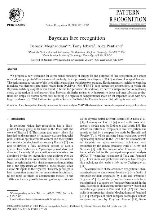
Bayesian face *, Tony Jebara , Alex Pentland
Mitsubishi Electric Research Laboratory, 201 Broadway, 8th yoor, Cambridge, MA 02139, USA Massachusettes Institute of Technology, Cambridge, MA 02139, USA Received 15 January 1999; received in revised form 28 July 1999; accepted 28 July 1999
1772
B. Moghaddam et al. / Pattern Recognition 33 (2000) 1771 } 1782
discriminant analysis (LDA) as used by Etemad and Chellappa [16], the `Fisherfacea technique of Belhumeur et al. [17], hierarchical discriminants used by Swets and Weng [18] and `evolutionary pursuita of optimal subspaces by Liu and Wechsler [19] * all of which have proved equally (if not more) powerful than standard `eigenfacesa. Eigenspace techniques have also been applied to modeling the shape (as opposed to texture) of the face. Eigenspace coding of shape-normalized or `shape-freea faces, as suggested by Craw and Cameron [20], is now a standard pre-processing technique which can enhance performance when used in conjunction with shape information [21]. Lanitis et al. [22] have developed an automatic face-processing system with subspace models of both the shape and texture components, which can be used for recognition as well as expression, gender and pose classi"cation. Additionally, subspace analysis has also been used for robust face detection [12,14,23], nonlinear facial interpolation [24], as well as visual learning for general object recognition [13,25,26].
基于eigenfaces的人脸识别算法实现大学论文

河北农业大学本科毕业论文(设计)题目:基于Eigenfaces的人脸识别算法实现摘要随着科技的快速发展,视频监控技术在我们生活中有着越来越丰富的应用。
在这些视频监控领域迫切需要一种远距离,非配合状态下的快速身份识别,以求能够快速识别所需要的人员信息,提前智能预警。
人脸识别无疑是最佳的选择。
可以通过人脸检测从视频监控中快速提取人脸,并与人脸数据库对比从而快速识别身份。
这项技术可以广泛应用于国防,社会安全,银行电子商务,行政办公,还有家庭安全防务等多领域。
本文按照完整人脸识别流程来分析基于PCA(Principal Component Analysis)的人脸识别算法实现的性能。
首先使用常用的人脸图像的获取方法获取人脸图像。
本文为了更好的分析基于PCA人脸识别系统的性能选用了ORL人脸数据库。
然后对人脸数据库的图像进行了简单的预处理。
由于ORL人脸图像质量较好,所以本文中只使用灰度处理。
接着使用PCA提取人脸特征,使用奇异值分解定理计算协方差矩阵的特征值和特征向量以及使用最近邻法分类器欧几里得距离来进行人脸判别分类。
关键词:人脸识别PCA算法奇异值分解定理欧几里得距离ABSTRACTWith the rapid development of technology, video surveillance technology has become increasingly diverse applications in our lives. In these video surveillance urgent need for a long-range, with rapid identification of non-state, in order to be able to quickly identify people the information they need, advance intelligence warning. Face recognition is undoubtedly the best choice. Face detection can quickly extract human faces from video surveillance, and contrast with the face database to quickly identify identity. This technology can be widely used in national defense, social security, bank e-commerce, administrative offices, as well as home security and defense and other areas.In accordance with the full recognition process to analyze the performance of PCA-based face recognition algorithm. The first to use the method of access to commonly used face images for face images. In order to better analysis is based on the performance of the PCA face recognition system selected ORL face database. Then the image face database for a simple pretreatment. Because ORL face image quality is better, so this article uses only gray scale processing. Then use the PCA for face feature extraction using singular value decomposition theorem to calculate the covariance matrix of the eigenvalues and eigenvectors, and use the Euclidean distance of the nearest neighbor classifier to the classification of human face discrimination.KEYWORDS: face recognition PCA algorithm SVD Euclidean distance目录摘要 (1)ABSTRACT (2)1 人脸识别概述 (4)1.1 人脸识别的研究概况和发展趋势 (4)1.1.1 人脸识别的研究概况 (4)1.1.2 人脸识别的发展趋势 (5)1.2 人脸识别的主要难点 (6)1.3 人脸识别的流程 (6)1.3.1 人脸图像采集 (7)1.3.2 预处理 (7)1.3.3 特征提取 (7)1.4 本章小结 (8)2 人脸图像 (9)2.1 人脸图像获取 (9)2.2 人脸图像数据库 (9)2.3 人脸图像预处理 (10)2.3.1 灰度变化 (10)2.3.2 二值化 (11)2.3.3 图像锐化 (11)2.4 本章小结 (12)3 人脸识别 (13)3.1 PCA算法理论 (13)3.2 PCA人脸识别算法的实现 (14)3.2.1 K-L变换 (14)3.2.2 SVD 定理 (14)3.2.3 PCA算法 (15)3.2.4 人脸识别过程 (16)3.3 程序运行效果 (16)3.4 程序代码 (17)3.4.1 代码类关系 (17)3.4.2 代码的OpenCV相关 (18)3.4.3 关键函数代码 (18)3.5 本章小结 (22)结论 (23)致谢 (24)参考文献 (25)1人脸识别概述1.1 人脸识别的研究概况和发展趋势1.1.1 人脸识别的研究概况人脸识别的研究开始于上世纪七十年代,当时的研究主要是基于人脸外部轮廓的方法。
Face Recognition Eigen-faces with 99 PCA coefficients
Results – Gender Classification
KNN
Male
Female
Accurac y
77.81% 23.07% 34.61% 4.63% 88.83% 67.95%
Overall Accuracy:
Overall Accuracy:
DiscussionDiscussion- Race Classification
Bad Data Issues
As it invariably happens with any real-world realproblem data base, this problem also contains few bad faces, missing faces and outliers. In the implementation here the faces with missing descriptors are taken out from the data base where as outliers and bad faces are kept as it is.
Summary of the Work
Parzen Window K- nearest neighborhood Generalized linear discriminant Neural network Boosting (neural nets as component classifiers) I have implemented all 5 Algorithms for almost all feature classification excluding Facial Expressions.
基于pca算法的eigenfaces人脸识别算法大学论文
河北农业大学现代科技学院毕业论文(设计)题目:基于PCA算法的Eigenfaces人脸识别算法摘要人脸识别技术就是利用计算机分析人脸图像,提取有效的识别信息来辨认身份或者判别待定状态的一门技术。
它涉及模式识别、图像处理、计算机视觉等诸多学科的知识,是当前研究的热点之一。
然而影响计算机人脸识别的因素非常之多,主要是人脸表情丰富,人脸随年龄增长而变化,人脸所成图像受光照、成像角度及成像距离等影响,极大地影响了人脸识别走向实用化。
基于PCA算法的人脸识别过程大致分为训练、测试、识别这三个阶段完成,在训练阶段,通过寻找协方差矩阵的特征向量,求出样本在该特征向量上的投影系数;在测试阶段,通过将测试样本投影到特征向量上,得到测试样本在该特征向量上的投影系数。
最后,采用最小欧氏距离,找到了与测试样本最相近的训练样本图像。
关键词Eigenfaces、PCA算法、人脸识别算法、matlab、SVD。
AbstractFace recognition technology is the use of computer analysis of facial images to extract valid identification information to identify or determine the identity of a technology Pending state. It involves knowledge of pattern recognition, image processing, computer vision, and many other disciplines, is one of the hotspots of current research. However, factors affecting the computer face recognition very much, mainly rich facial expression, face changes with age, face a picture of the affected light, imaging and imaging distance, angle, greatly influenced the Face to practical use.PCA algorithm based recognition process is roughly divided into training and testing, the identification of these three stages, in the training phase, to find the eigenvectors of the covariance matrix is obtained on the sample feature vector projection coefficient; in the test phase by the test feature vector is projected onto the sample to obtain a test sample on the projection of the feature vector of coefficients.Finally, the minimum Euclidean distance, the test sample to find the closest sample images.Keywords Eigenfaces PCA Algorithm、Face Recognition Algorithm、matlab、SVD.目录1 绪论---------------------------------------------------------------------- 11.1计算机人脸识别技术及应用--------------------------------------------- 11.2常用的人脸识别方法简介----------------------------------------------- 11.3本论文内容安排------------------------------------------------------- 12 PCA ----------------------------------------------------------------------- 32.1 PCA简介------------------------------------------------------------- 32.2 PCA的实质----------------------------------------------------------- 32.3 PCA理论基础--------------------------------------------------------- 32.3.1投影----------------------------------------------------------- 32.3.2最小平方误差理论----------------------------------------------- 42.3.3 PCA几何解释--------------------------------------------------- 82.4 PCA降维计算--------------------------------------------------------- 83 PCA在人脸识别中的应用--------------------------------------------------- 113.1 人脸识别技术简介--------------------------------------------------- 113.2 图片归一化--------------------------------------------------------- 113.3 基于PCA的人脸识别------------------------------------------------- 113.3.1 人脸数据特征提取---------------------------------------------- 113.3.2计算均值------------------------------------------------------ 123.3.3计算协方差矩阵C ----------------------------------------------- 123.3.4求出协方差C的特征值和特征向量-------------------------------- 123.4奇异值分解定理------------------------------------------------------ 123.5 基于PCA的人脸识别的训练------------------------------------------- 133.5.1 训练集的主成分计算-------------------------------------------- 133.5.2 训练集图片重建------------------------------------------------ 133.6 识别--------------------------------------------------------------- 144 实验--------------------------------------------------------------------- 154.1 实验环境----------------------------------------------------------- 154.2 PCA人脸识别实验过程------------------------------------------------ 154.2.1 训练阶段------------------------------------------------------ 154.2.2 测试阶段------------------------------------------------------ 224.2.3 采用欧氏最小距离识别------------------------------------------ 234.3实验结果------------------------------------------------------------ 245 总结--------------------------------------------------------------------- 265.1.1内容总结:---------------------------------------------------- 265.1.2工作总结:---------------------------------------------------- 26 6致谢--------------------------------------------------------------------- 27 参考文献------------------------------------------------------------------- 281 绪论1.1计算机人脸识别技术及应用计算机人脸识别技术就是利用计算机分析人脸图像,进而从中提取出有效的识别信息,用来“辨认”身份的一门技术,它涉及图像处理、模式识别、计算机视觉、神经网络、生理学、心理学等诸多学科领域的知识。
基于PCA和图像分块加权的人脸识别方法
摘要:鉴于人脸的表情变化时人脸的不同部位变化的程度大小不同,本文提出了人脸分块加权和主元分析(PCA,Principal Compo-nent Analysis)相结合的识别方法。
关键词:人脸识别PCA 图像矩阵子图像人脸识别技术作为一种既方便快捷又安全可靠的身份认证手段,被广泛应用于诸多领域。
根据人脸识别技术的特征和分类差异可将其分为以下三种类型:提取人脸几何特征的方法、基于特征分析的模板匹配、统计分析的方法。
其中,基于主元分析的本征脸法,因其计算程序简单和准确率高,受到了使用者的一致欢迎。
1主元分析(PCA)方法主元分析法又称本征脸法,是人脸识别技术中最常用的一种方法。
在使用时,使用者采用PCA 方法来表征被测试者的人脸图像,所得到的任意一幅图像都可以用一组本征脸的线性加权和来近似重构。
而要想获得这一组本征脸的权重系数,使用者需对此进行空间投影。
M.Turk 和A.Pentland 将PCA 方法应用于人脸识别和检测中,取得了极大成功。
其工作原理如下:假设训练图像按行叠成长度为N 的矢量Γ1,Γ2,…,ΓM ,其均值矢量(即平均脸)为Ψ=1M Mi =1∑Γi,则每个图像相对于均值图像的差为Φi =Γi -Ψ(i=1,2,…,M)。
令矩阵A=[Φ1,Φ2,…,ΦM ],则散布矩阵∑可以表示为:∑=AA T ≅1M Mi =1∑Φi ΦT i (1)求出∑的本征值λk 和本征矢量u k 。
由于u k 看起来像一张人脸,因此u k 称作本征矢量。
由于∑是N×N 的矩阵,而且N 的值较大,一般远大于训练样本的个数M,因此,为了降低计算量,通常不直接求∑的本征矢量u k ,而是先计算大小为M×M 的矩阵A T A 的本征矢量v k ,然后,根据代数理论,有u k =1λk√Av k(2)按照这些相互正交的本征矢量对应的本征值大小顺序进行排列,根据从前到后的顺序进行取值,任取J(J<M)个本征矢量,将其作为主元建立一个本征空间S。
英文翻译
成都信息工程学院毕业设计英文翻译介绍了人脸检测和人脸识别系别电子工程学院姓名王雄专业电子信息工程班级信号处理2班学号2010021176Introduction to Face Detection and Face RecognitionLast updated on 4th Feb, 2012 by Shervin Emami. Posted originally on 2nd June, 2010."Face Recognition" is a very active area in the Computer Vision and Biometrics fields, as it has been studied vigorously for 25 years and is finally producing applications in security, robotics, human-computer-interfaces, digital cameras, games and entertainment."Face Recognition" generally involves two stages:Face Detection, where a photo is searched to find any face (shown here as a green rectangle), then image processing cleans up the facial image for easier recognition. Face Recognition, where that detected and processed face is compared to a database of known faces, to decide who that person is (shown here as red text).Since 2002, Face Detection can be performed fairly reliably such as with OpenCV's Face Detector, working in roughly 90-95% of clear photos of a person looking forward at the camera. It is usually harder to detect a person's face when they are viewed from the side or at an angle, and sometimes this requires 3D Head Pose Estimation. It can also be very difficult to detect a person's face if the photo is not very bright, or if part of the face is brighter than another or has shadows or is blurry or wearing glasses, etc. However, Face Recognition is much less reliable than Face Detection, generally 30-70% accurate. Face Recognition has been a strong field of research since the 1990s, but is still far from reliable, and more techniques are being invented each year such as the ones listed at the bottom of this page (Alternatives to Eigenfaces such as 3D face recognition or recognition from video).I will show you how to use Eigenfaces (also called "Principal Component Analysis" or PCA), a simple and popular method of 2D Face Recognition from a photo, as opposed to other common methods such as Neural Networks orFisher Faces.To learn the theory of how Eigenface works, you should read Face Recognition With Eigenface from Servo Magazine (April 2007), and perhaps the mathematical algorithm. First I will explain how to implement Eigenfaces for offline training from the command-line, based on the Servo Magazine tutorial and source-code (May 2007). Once I have explained to you how offline training and offline face recognition works from the command-line, I will explain how this can be extended to online training directly from a webcam in realtime :-)How to detect a face using OpenCV's Face Detector:As mentioned above, the first stage in Face Recognition is Face Detection. The OpenCV library makes it fairly easy to detect a frontal face in an image using its Haar Cascade Face Detector (also known as the Viola-Jones method).The function "cvHaarDetectObjects" in OpenCV performs the actual face detection, but the function is a bit tedious to use directly, so it is easiest to use this wrapper function: // Perform face detection on the input image, using the given Haar Cascade. // Returns a rectangle for the detected region in the given image.CvRect detectFaceInImage(IplImage *inputImg, CvHaarClassifierCascade* cascade) {// Smallest face size.CvSize minFeatureSize = cvSize(20, 20);// Only search for 1 face.int flags = CV_HAAR_FIND_BIGGEST_OBJECT | CV_HAAR_DO_ROUGH_SEARCH;// How detailed should the search be.float search_scale_factor = 1.1f;IplImage *detectImg;IplImage *greyImg = 0;CvMemStorage* storage;CvRect rc;double t;CvSeq* rects;CvSize size;int i, ms, nFaces;storage = cvCreateMemStorage(0);cvClearMemStorage( storage );// If the image is color, use a greyscale copy of the image.detectImg = (IplImage*)inputImg;if (inputImg->nChannels > 1) {size = cvSize(inputImg->width, inputImg->height);greyImg = cvCreateImage(size, IPL_DEPTH_8U, 1 );cvCvtColor( inputImg, greyImg, CV_BGR2GRAY );detectImg = greyImg; // Use the greyscale image.}// Detect all the faces in the greyscale image.t = (double)cvGetTickCount();rects = cvHaarDetectObjects( detectImg, cascade, storage,search_scale_factor, 3, flags, minFeatureSize);t = (double)cvGetTickCount() - t;ms = cvRound( t / ((double)cvGetTickFrequency() * 1000.0) );nFaces = rects->total;printf("Face Detection took %d ms and found %d objects\n", ms, nFaces);// Get the first detected face (the biggest).if (nFaces > 0)rc = *(CvRect*)cvGetSeqElem( rects, 0 );elserc = cvRect(-1,-1,-1,-1); // Couldn't find the face.if (greyImg)cvReleaseImage( &greyImg );cvReleaseMemStorage( &storage );//cvReleaseHaarClassifierCascade( &cascade );return rc; // Return the biggest face found, or (-1,-1,-1,-1).}Now you can simply call "detectFaceInImage" whenever you want to find a face in an image. You also need to specify the face classifier that OpenCV should use to detect the face. For example, OpenCV comes with several different classifiers for frontal face detection, as well as some profile faces (side view), eye detection, nose detection, mouth detection, whole body detection, etc. You can actually use this function with any of these other detectors if you want, or even create your own custom detector such as for car or person detection (read here), but since frontal face detection is the only one that is very reliable, it is the only one I will discuss.For frontal face detection, you can chose one of these Haar Cascade Classifiers that come with OpenCV (in the "data\haarcascades\" folder):"haarcascade_frontalface_default.xml""haarcascade_frontalface_alt.xml""haarcascade_frontalface_alt2.xml""haarcascade_frontalface_alt_tree.xml"Each one will give slightly different results depending on your environment, so you could even use all of them and combine the results together (if you want the most detections). There are also some more eye, head, mouth and nose detectors in the downloads section of Modesto's page.So you could do this in your program for face detection:// Haar Cascade file, used for Face Detection.char *faceCascadeFilename ="haarcascade_frontalface_alt.xml";// Load the HaarCascade classifier for face detection.CvHaarClassifierCascade* faceCascade;faceCascade = (CvHaarClassifierCascade*)cvLoad(faceCascadeFilename, 0, 0, 0);if( !faceCascade ) {printf("Couldnt load Face detector '%s'\n", faceCascadeFilename);exit(1);}// Grab the next frame from the camera.IplImage *inputImg = cvQueryFrame(camera);// Perform face detection on the input image, using the given Haar classifierCvRect faceRect = detectFaceInImage(inputImg, faceCascade);// Make sure a valid face was detected.if (faceRect.width > 0) {printf("Detected a face at (%d,%d)!\n", faceRect.x, faceRect.y);}.... Use 'faceRect' and 'inputImg' ....// Free the Face Detector resources when the program is finished cvReleaseHaarClassifierCascade( &cascade );How to preprocess facial images for Face Recognition:Now that you have detected a face, you can use that face image for Face Recognition. However, if you tried to simply perform face recognition directly on a normal photo image, you will probably get less than 10% accuracy!It is extremely important to apply various image pre-processing techniques to standardize the images that you supply to a face recognition system. Most face recognition algorithms are extremely sensitive to lighting conditions, so that if it was trained to recognize a person when they are in a dark room, it probably wont recognize them in a bright room, etc. This problem is referred to as "lumination dependent", and there are also many other issues, such as the face should also be in a very consistent position within the images (such as the eyes being in the same pixel coordinates), consistent size, rotation angle, hair and makeup, emotion (smiling, angry, etc), position of lights (to the left or above, etc). This is why it is so important to use a good image preprocessing filters before applying face recognition. You should also do things like removing the pixels around the face that aren't used, such as with an elliptical mask to only show the inner face region, not the hair and image background, since they change more than the face does.For simplicity, the face recognition system I will show you is Eigenfaces using greyscale images. So I will show you how to easily convert color images to greyscale (also called 'grayscale'), and then easily apply Histogram Equalization as a very simplemethod of automatically standardizing the brightness and contrast of your facial images. For better results, you could use color face recognition (ideally with color histogram fitting in HSV or another color space instead of RGB), or apply more processing stages such as edge enhancement, contour detection, motion detection, etc. Also, this code is resizing images to a standard size, but this might change the aspect ratio of the face. You can read my tutorial HERE on how to resize an image while keeping its aspect ratio the same.Here you can see an example of this preprocessing stage:Here is some basic code to convert from a RGB or greyscale input image to a greyscale image, resize to a consistent dimension, then apply Histogram Equalization for consistent brightness and contrast:// Either convert the image to greyscale, or use the existing greyscale image. IplImage *imageGrey;if (imageSrc->nChannels == 3) {imageGrey = cvCreateImage( cvGetSize(imageSrc), IPL_DEPTH_8U, 1 );// Convert from RGB (actually it is BGR) to Greyscale.cvCvtColor( imageSrc, imageGrey, CV_BGR2GRAY );}else {// Just use the input image, since it is already Greyscale.imageGrey = imageSrc;}// Resize the image to be a consistent size, even if the aspect ratio changes.IplImage *imageProcessed;imageProcessed = cvCreateImage(cvSize(width, height), IPL_DEPTH_8U, 1);// Make the image a fixed size. // CV_INTER_CUBIC or CV_INTER_LINEAR is good for enlarging, and // CV_INTER_AREA is good for shrinking / decimation, but bad at enlarging.cvResize(imageGrey, imageProcessed, CV_INTER_LINEAR);// Give the image a standard brightness and contrast.cvEqualizeHist(imageProcessed, imageProcessed);..... Use 'imageProcessed' for Face Recognition ....if (imageGrey)cvReleaseImage(&imageGrey);if (imageProcessed)cvReleaseImage(&imageProcessed);How Eigenfaces can be used for Face Recognition:Now that you have a pre-processed facial image, you can perform Eigenfaces (PCA) for Face Recognition. OpenCV comes with the function "cvEigenDecomposite()", which performs the PCA operation, however you need a database (training set) of images for it to know how to recognize each of your people.So you should collect a group of preprocessed facial images of each person you want to recognize. For example, if you want to recognize someone from a class of 10 students, then you could store 20 photos of each person, for a total of 200 preprocessed facial images of the same size (say 100x100 pixels).The theory of Eigenfaces is explained in the two Face Recognition with Eigenface articles in Servo Magazine, but I will also attempt to explain it here.Use "Principal Component Analysis" to convert all your 200 training images into a set of "Eigenfaces" that represent the main differences between the training images. First it will find the "average face image" of your images by getting the mean value of each pixel. Then the eigenfaces are calculated in comparison to this average face, where the first eigenface is the most dominant face differences, and the second eigenface is the second most dominant face differences, and so on, until you have about 50 eigenfaces that represent most of the differences in all the training set images.In these example images above you can see the average face and the first and last eigenfaces that were generated from a collection of 30 images each of 4 people. Notice that the average face will show the smooth face structure of a generic person, the first few eigenfaces will show some dominant features of faces, and the last eigenfaces (eg: Eigenface 119) are mainly image noise. You can see the first 32 eigenfaces in the image below.Explanation of Face Recognition using Principal Component Analysis:To explain Eigenfaces (Principal Component Analysis) in simple terms, Eigenfaces figures out the main differences between all the training images, and then how to represent each training image using a combination of those differences.So for example, one of the training images might be made up of:(averageFace) + (13.5% of eigenface0) - (34.3% of eigenface1) + (4.7% of eigenface2) + ... + (0.0% of eigenface199).Once it has figured this out, it can think of that training image as the 200 ratios: {13.5, -34.3, 4.7, ..., 0.0}.It is indeed possible to generate the training image back from the 200 ratios by multiplying the ratios with the eigenface images, and adding the average face. But since many of the last eigenfaces will be image noise or wont contribute much to the image, this list of ratios can be reduced to just the most dominant ones, such as the first 30 numbers, without effecting the image quality much. So now its possible to represent all 200 training images using just 30 eigenface images, the average face image, and a list of 30 ratios for each of the 200 training images.Interestingly, this means that we have found a way to compress the 200 images into just 31 images plus a bit of extra data, without loosing much image quality. But this tutorial is about face recognition, not image compression, so we will ignore that :-)To recognize a person in a new image, it can apply the same PCA calculations to find 200 ratios for representing the input image using the same 200 eigenfaces. And once again it can just keep the first 30 ratios and ignore the rest as they are less important. It can then search through its list of ratios for each of its 20 known people in its database, to see who has their top 30 ratios that are most similar to the 30 ratios for the input image. This is basically a method of checking which training image is most similar to the input image, out of the whole 200 training images that were supplied. Implementing Offline Training:For implementation of offline training, where files are used as input and output through the command-line, I am using a similar method as the Face Recognition with Eigenface implementation in Servo Magazine, so you should read that article first, but I have made a few slight changes.Basically, to create a facerec database from training images, you create a text file that lists the image files and which person each image file represents.For example, you could put this into a text file called "4_images_of_2_people.txt":1 Shervindata\Shervin\Shervin1.bmp1 Shervindata\Shervin\Shervin2.bmp1 Shervindata\Shervin\Shervin3.bmp1 Shervindata\Shervin\Shervin4.bmp2 Chandandata\Chandan\Chandan1.bmp2 Chandandata\Chandan\Chandan2.bmp2 Chandandata\Chandan\Chandan3.bmp2 Chandandata\Chandan\Chandan4.bmpThis will tell the program that person 1 is named "Shervin", and the 4 preprocessedfacial photos of Shervin are in the "data\Shervin" folder, and person 2 is called "Chandan" with 4 images in the "data\Chandan" folder. The program can then loaded them all into an array of images using the function "loadFaceImgArray()". Note that for simplicity, it doesn't allow spaces or special characters in the person's name, so you might want to enable this, or replace spaces in a person's name with underscores (such as Shervin_Emami).To create the database from these loaded images, you use OpenCV's "cvCalcEigenObjects()" and "cvEigenDecomposite()" functions, eg:// Tell PCA to quit when it has enough eigenfaces.CvTermCriteria calcLimit = cvTermCriteria( CV_TERMCRIT_ITER, nEigens, 1);// Compute average image, eigenvectors (eigenfaces) and eigenvalues (ratios).cvCalcEigenObjects(nTrainFaces, (void*)faceImgArr, (void*)eigenVectArr, CV_EIGOBJ_NO_CALLBACK, 0, 0, &calcLimit,pAvgTrainImg, eigenValMat->data.fl);// Normalize the matrix of eigenvalues.cvNormalize(eigenValMat, eigenValMat, 1, 0, CV_L1, 0);// Project each training image onto the PCA subspace.CvMat projectedTrainFaceMat = cvCreateMat( nTrainFaces, nEigens, CV_32FC1 );int offset = projectedTrainFaceMat->step / sizeof(float);for(int i=0; i<nTrainFaces; i++) {cvEigenDecomposite(faceImgArr[i], nEigens, eigenVectArr, 0, 0,pAvgTrainImg, projectedTrainFaceMat->data.fl + i*offset);}You now have:the average image "pAvgTrainImg",the array of eigenface images "eigenVectArr[]" (eg: 200 eigenfaces if you used nEigens=200 training images),the matrix of eigenvalues (eigenface ratios) "projectedTrainFaceMat" of each training image.These can now be stored into a file, which will be the face recognition database. The function "storeTrainingData()" in the code will store this data into the file "facedata.xml", which can be reloaded anytime to recognize people that it has beentrained for. There is also a function "storeEigenfaceImages()" in the code, to generate the images shown earlier, of the average face image to "out_averageImage.bmp" and eigenfaces to "out_eigenfaces.bmp".Implementing Offline Recognition:For implementation of the offline recognition stage, where the face recognition system will try to recognize who is the face in several photos from a list in a text file, I am also using an extension of the Face Recognition with Eigenface implementation in Servo Magazine.The same sort of text file that is used for offline training can also be used for offline recognition. The text file lists the images that should be tested, as well as the correct person in that image. The program can then try to recognize who is in each photo, and check the correct value in the input file to see whether it was correct or not, for generating statistics of its own accuracy.The implementation of the offline face recognition is almost the same as offline training:The list of image files (preprocessed faces) and names are loaded into an array of images, from the text file that is now used for recognition testing (instead of training). This is performed in code by "loadFaceImgArray()".The average face, eigenfaces and eigenvalues (ratios) are loaded from the face recognition database file "facedata.xml", by the function "loadTrainingData()".Each input image is projected onto the PCA subspace using the OpenCV function "cvEigenDecomposite()", to see what ratio of eigenfaces is best for representing this input image.But now that it has the eigenvalues (ratios of eigenface images) to represent the input image, it looks for the original training image that had the most similar ratios. This is done mathematically in the function "findNearestNeighbor()" using the "Euclidean Distance", but basically it checks how similar the input image is to each training image, and finds the most similar one: the one with the least distance in Euclidean Space. As mentioned in the Servo Magazine article, you might get better results if you use the Mahalanobis space (define USE_MAHALANOBIS_DISTANCE in the code).The distance between the input image and most similar training image is used to determine the "confidence" value, to be used as a guide of whether someone wasactually recognized or not. A confidence of 1.0 would mean a good match, and a confidence of 0.0 or negative would mean a bad match. But beware that the confidence formula I use in the code is just a very basic confidence metric that isn't necessarily too reliable, but I figured that most people would like to see a rough confidence value. You may find that it gives misleading values for your images and so you can disable it if you want (eg: set the confidence always to 1.0).Once it knows which training image is most similar to the input image, and assuming the confidence value is not too low (it should be atleast 0.6 or higher), then it has figured out who that person is, in other words, it has recognized that person! Implementing Realtime Recognition from a Camera:It is very easy to use a webcam stream as input to the face recognition system instead of a file list. Basically you just need to grab frames from a camera instead of from a file, and you run forever until the user wants to quit, instead of just running until the file list has run out. OpenCV provides the 'cvCreateCameraCapture()' function (also known as 'cvCaptureFromCAM()') for this.Grabbing frames from a webcam can be implemented easily using this function:// Grab the next camera frame. Waits until the next frame is ready, and // provides direct access to it, so do NOT modify or free the returned image! // Will automatically initialize the camera on the first frame.IplImage* getCameraFrame(CvCapture* &camera){IplImage *frame;int w, h;// If the camera hasn't been initialized, then open it.if (!camera) {printf("Acessing the camera ...\n");camera = cvCreateCameraCapture( 0 );if (!camera) {printf("Couldn't access the camera.\n");exit(1);}// Try to set the camera resolution to 320 x 240.cvSetCaptureProperty(camera, CV_CAP_PROP_FRAME_WIDTH, 320);cvSetCaptureProperty(camera, CV_CAP_PROP_FRAME_HEIGHT, 240);// Get the first frame, to make sure the camera is initialized.frame = cvQueryFrame( camera );if (frame) {w = frame->width;h = frame->height;printf("Got the camera at %dx%d resolution.\n", w, h);}// Wait a little, so that the camera can auto-adjust its brightness.Sleep(1000); // (in milliseconds)}// Wait until the next camera frame is ready, then grab it.frame = cvQueryFrame( camera );if (!frame) {printf("Couldn't grab a camera frame.\n");exit(1);}return frame;}This function can be used like this:CvCapture* camera = 0; // The camera device.while ( cvWaitKey(10) != 27 ) { // Quit on "Escape" key.IplImage *frame = getCameraFrame(camera);...}// Free the camera.cvReleaseCapture( &camera );Note that if you are developing for MS Windows, you can grab camera frames twice as fast as this code by using the videoInput Library v0.1995 by Theo Watson. It uses hardware-accelerated DirectShow, whereas OpenCV uses VFW that hasn't changed in 15 years!Putting together all the parts that I have explained so far, the face recognition systemruns as follows:Grab a frame from the camera (as I mentioned here).Convert the color frame to greyscale (as I mentioned here).Detect a face within the greyscale camera frame (as I mentioned here).Crop the frame to just show the face region (using cvSetImageROI() and cvCopyImage()).Preprocess the face image (as I mentioned here).Recognize the person in the image (as I mentioned here).Implementing Online Training from a Camera:Now you have a way to recognize people in realtime using a camera, but to learn new faces you would have to shutdown the program, save the camera images as image files, update the training images list, use the offline training method from the command-line, and then run the program again in realtime camera mode. So in fact, this is exactly what you can do programmatically to perform online training from a camera in realtime!So here is the easiest way to add a new person to the face recognition database from the camera stream without shutting down the program:Collect a bunch of photos from the camera (preprocessed facial images), possibly while you are performing face recognition also.Save the collected face images as image files onto the hard-disk using cvSaveImage().Add the filename of each face image onto the end of the training images list file (the text file that is used for offline training).Once you are ready for online training the new images (such as once you have 20 faces, or when the user says that they are ready), you "retrain" the database from all the image files. The text file listing the training image files has the new images added to it, and the images are stored as image files on the computer, so online training works just like it did in offline training.But before retraining, it is important to free any resources that were being used, and re-initialize the variables, so that it behaves as if you shutdown the program and restarted. For example, after the images are stored as files and added to the training list text file, you should free the arrays of eigenfaces, before doing the equivalent of offline training (which involves loading all the images from the training list file, then findingthe eigenfaces and ratios of the new training set using PCA).This method of online training is fairly inefficient, because if there was 50 people in the training set and you add one more person, then it will train again for all 51 people, which is bad because the amount of time for training is exponential with more users or training images. But if you are just dealing with a few hundred training images in total then it shouldn't take more than a few seconds.Download OnlineFaceRec:The software and source-code is available here (open-source freeware), to use on Windows, Mac, Linux, iPhone, etc as you wish for educational or personal purposes, but NOT for commercial, criminal-detection, or military purposes (because this code is way too simple & unreliable for critical applications such as criminal detection, and also I no longer support any military).Click here to download "OnlineFaceRec" for Windows: onlineFaceRec.zip(0.07MB file including C/C++ source code, VS2008 project files and the compiled Win32 program, created 4th Feb 2012).Click here to download "OnlineFaceRec" for Linux: onlineFaceRec_Linux.zip(0.003MB file including C/C++ source code and a compiled Linux program, created 30th Dec 2011).If you dont have the OpenCV 2.0 SDK then you can just get the Win32 DLLs and HaarCascade for running this program (including 'cvaux200.dll' and 'haarcascade_frontalface_alt.xml'): onlineFaceRec_OpenCVbinaries.7z (1.7MB 7-Zip file).And if you want to run the program but dont have the Visual Studio 2008 runtime installed then you can just get the Win32 DLLs ('msvcr90.dll', etc): MS_VC90_CRT.7z (0.4MB 7-Zip file).To open Zip or 7z files you can use the freeware 7-Zip program (better than WinZip and WinRar in my opinion) from HERE.The code was tested with MS Visual Studio 2008 using OpenCV v2.0 and on Linux with GCC 4.2 using OpenCV v2.3.1, but I assume it works with other versions & compilers fairly easily, and it should work the same in all versions of OpenCV before v2.2. Students also ported this code to Dev-C++ athttps:///projects/facerec/.There are two different ways you can use this system:As a realtime program that performs face detection and online face recognition from a web camera.As a command-line program to perform offline face recognition using text files, just like the eigenface program in Servo Magazine.How to use the realtime webcam FaceRec system:If you have a webcam plugged in, then you should be able to test this program by just double-clicking the EXE file in Windows (or compile the code and run it if you are using Linux or Mac). Hit the Escape key on the GUI window when you want to quit the program.After a few seconds it should show the camera image, with the detected face highlighted. But at first it wont have anyone in its face rec database, so you will need to create it by entering a few keys. Beware that to use the keyboard, you have to click on the DOS console window before typing anything (because if the OpenCV window is highlighted then the code wont know what you typed).In the console window, hit the 'n' key on your keyboard when a person is ready for training. This will add a new person to the facerec database. Type in the person's name (without any spaces) and hit Enter.It will begin to automatically store all the processed frontal faces that it sees. Get a person to move their head around a bit until it has stored about 20 faces of them. (The facial images are stored as PGM files in the "data" folder, and their names are appended to the text file "train.txt").Get the person in front of the camera to move around a little and move their face a little, so that there will be some variance in the training images.Then when you have enough detected faces for that person, ideally more than 30 for each person, hit the 't' key in the console window to begin training on the images that were just collected. It will then pause for about 5-30 seconds (depending on how many faces and people are in the database), and finally continue once it has retrained with the extra person. The database file is called "facedata.xml".It should print the person's name in the console whenever it recognizes them. Repeat this again from step 1 whenever you want to add a new person, even after you have shutdown the program.。
外文1
Face Recognition Using EigenfacesAbstractWe present an approach to the detection and identification of human faces and describe a working, near-real-time face recognition system which tracks a subject’s head and then recognizes the person by comparing characteristics of the face to those of known individuals. Our approach treats face recognition as a two-dimensional recognition problem, taking advantage of the fact that faces are are normally upright and thus may be described by a small set of 2-D characteristic views.Face images are projected onto a feature space (“face space”)that best encodes the variation among known face images.The face space is defined by the “eigenfaces”, which are the eigenvectors of the set of faces;they do not necessarily correspond to isolated features such as eyes, ears, and noses.The framework provides the ability to learn to recognize new faces in an unsupervised manner.1 IntroductionDeveloping a computational model of face recognition is quite difficult, because faces are complex, multidimensional, and meaningful visual stimuli. They are a natural class of objects, and stand in stark contrast to sine wave gratings, the “blocks world”, and other artificial stimuli used in human and computer vision research[l]. Thus unlike most early visual functions, for which we may construct detailed models of retinal or striate activity,face recognition is a very high level task for which computational approaches can currently only suggest broad constraints on the corresponding neural activityWe therefore focused our research towards developing a sort of early, preattentive pattern recognition capability that does not depend upon having full three-dimensional models or detailed geometry.Our aim was to develop a computational model of face recognition which is fast, reasonably simple, and accurate in constrained environments such as an office or a household.Although face recognition is a high level visual problem, there is quite a bit of structure imposed on the task. We take advantage of some of this structure by proposing a scheme for recognition which is based on an information theory approach, seeking to encode the most relevant information in a group of faces which will best distinguish them from one another.The approach transforms face images into a small set of characteristic feature images, called “eigenfaces”,which are the principalcomponents of the initial training set of face images. Recognition is performed by projecting a new image into the subspace spanned by the eigenfa ces (“face space”) and then classifying the face by comparing its position in face space with the positions of known individuals.Automatically learning and later recognizing new faces is practical within this framework. Recognition under reasonably varying conditions is achieved by training on a limited number of characteristic views (e.g., a “straight on” view, a 45’ view, and a profile view).The approach has advantages over other face recognition schemes in its speed and simplicity, learning capacity, and relative insensitivity to small or gradual changes in the face image.1.1 Background and related workMuch of the work in computer recognition of faces has focused on detecting individual features such as the eyes, nose, mouth, and head outline, and defining a face model by the position, size, and relationships among these features.Beginning with Bledsoe’s[2]and Kanade’s[3]early systems, a number of automated or semi-automated face recognition strategies have modeled and classified faces based on normalized distances and ratios among feature points.Recently this general approach has been continued and improved by the recent work of Yuilleet al.[4].Such approaches have proven difficult to extend to multiple views, and have often been quite fragile. Research in human strategies of face recognition, moreover,has shown that individual features and their immediate relationships comprise an insufficient representation to account for the performance of adult human face identification [5].Nonetheless, this approach to face recognition remains the most popular one in the computer vision literature.Connectionist approaches to face identification seek to capture the configurationally, or gestalt-like nature of the task. Fleming and Cottrell [6], building on earlier work by Kohonen and Lahtio [7], use nonlinear units to train a network via back propagation to classify face images. Stoneham’s WISARD system [8] has been applied with some success to binary face images, recognizing both identity and expression.Most connectionist systems dealing with faces treat the input image as a general 2-D pattern, and can make no explicit use of the configurational properties of a face.Only very simple systems have been explored to date, and it is unclear how they will scale to larger problems.Recent work by Burt et al. [9] uses a “smart sensing” approach based on multiresolution template matching.The face models are built by hand from faceimages.2 Eigenfaces for RecognitionMuch of the previous work on automated face recognition has ignored the issue of just what aspects of the face stimulus are important for identification,assuming that predefined measurements were relevant and sufficient.This suggested to us that an information theory approach of coding and decoding face images may give insight into the information content of face images, emphasizing the significant local and global “features”.Such features may or may not be directly related to our intuitive notion of face features such as the eyes, nose, lips, and hair.In the language of information theory, we want to extract the relevant information in a face image,encode it as efficiently as possible, and compare one face encoding with a database of models encoded similarly.A simple approach to extracting the information contained in an image of a face is to somehow capture the variation in a collection of face images, independent of any judgment of features, and use this information to encode and compare individual face images.In mathematical terms, we wish to find the principal components of the distribution of faces, or the eigenvectors of the covariance matrix of the set of face images.These eigenvectors can be thought of as a set of features which together characterize the variation between face images.Each image location contributes more or less to each eigenvector, so that we can display the eigenvector as a sort of ghostly face which we call an eigenface.Some of these faces are shown in Figure 2.Each face image in the training set can be represented exactly in terms of a linear combination of the eigenfaces.The number of possible eigenfaces is equal to the number of face images in the training set. However the faces can also be approximated using only the “best” eigenfaces - those that have the largest eigenvalues, and which therefore account for the most variance within the set of face images.The primary reason for using fewer eigenfaces is computational efficiency, The best M’ eigenfaces span an M’-dimensional subspace ~ “face space” ~ of all possible images.As sinusoids of varying frequency and phase are the basis functions of a Fourier decomposition (and are in fact eigenfunctions of linear systems), the eigenfaces are the basis vectors of the eigenface decomposition.They argued that a collection of face images can be approximately reconstructed by storing a small collection of weights for each face and a small set of standard pictures.It occurred to us that if a multitude of face images can be reconstructed by weighted sums of a smallcollection of characteristic images,then an efficient way to learn and recognize faces might be to build the characteristic features from known face images and to recognize particular faces by comparing the feature weights needed to (approximately) reconstruct them with the weights associated with the known individuals.The following steps summarize the recognition process:1.Initialization: Acquire the training set of face images and calculate the eigenfaces, which define the face space.2.When a new face image is encountered, calculate a set of weights based on the input image and the M eigenfaces by projecting the input image onto each of the eigenfaces.3.Determine if the image is a face at all (whether known or unknown) by checking to see if the image is sufficiently close to “face space.”4.If it is a face, classify the weight pattern as either a known person or as unknown.5.(Optional) If the same unknown face is seen several times, calculate its characteristic weight pattern and incorporate into the known faces(i.e., learn to recognize it).2.1 Calculating EigenfacesLet a face image 1(z, y) be a two-dimensional N by N array of intensity values, or a vector of dimension N.A typical image of size 256 by 256 describes a vector of dimension 65,536, or, equivalently, a point in 65,536-dimensional space.An ensemble of images, then, maps to a collection of points in this huge space.Images of faces, being similar in overall configuration, will not be randomly distributed in this huge image space and thus can be described by a relatively low dimensional subspace.The main idea of the principal component analysis (or Karhunen-Loeve expansion) is to find the vectors which best account for the distribution of face images within the entire image space.These vectors define the subspace of face images, which we call “face spa ce”. Each vector is of length N2 , describes an N by N image, and is a linear combination of the original face images.Because these vectors are the eigenvectors of the covariance matrix corresponding to the original face images, and because they are face-li ke in appearance, we refer to them as “eigenfaces.”Figure 1: (a) Face images used as the training set, (b) The average face Ψ.Let the training set of face images be T 1T 2T 3……T M ,The average face of the set is defined by Ψ =11M n n T M =∑. Each face differs from the average by the vector Φi =T i –Ψ An example training set is shown in Figure l (a) , with the average face Ψ shown in Figure l(b). This set of very large vectors is then subject to principal component analysis. Which seeks a set of M orthonormal vectors u n and their associated eigenvalues λk which best describes the distribution of the data. The vectors u k and scalars λk are the eigenvectors and eigenvalues. Respectively of the covariance matrix. C = 11M T n n n M =ΦΦ∑ Where the matrix A = [Φ1Φ2…Φ3], The matrix C, however, is N 2 by N 2, and determining the N 2 eigenvectors and eigenvalues is an intractable task for typical image sizes. We need a computationally feasible method to find these eigenvectors. Fortunately we can determine the eigenvectors by first solving a much smaller M byM matrix problem. And taking linear combinations of the resulting vectors. (See [ll] for the details.)With this analysis the calculations are greatly reduced from the order of the number of pixels in the images(N2)to the order of the number of images in the training set(M),In practice. the training set of face images will tie relatively small (M 《N2).and the calculation become quite manageable.The associated eigenvalues allow us to rank the eigenvectors according to their usefulness in characterizing the variation among the images.Figure 2 shows the top seven eigenfaces derived from the input images of Figure 1. Normally the background is removed by cropping training images. so that the eigenfaces have zero values outside of the face area.Figure 2: Seven of the eigenfaces calculated from the images of Figure 1, without the background removed.2.2 Using Eigenfaces to classify a face imageOnce the eigenfaces are created identification becomes a pattern recognition task. The eigenfaces span an M’-dimensional subspace of the original N2image space.The M’ significant eigenvectors of the L matrix are chosen as those with the largest associated eigenvalues.In many of our test cases based on M = 16 face images M’ =7 eigenfaces were used.The number of eigenfaces to be used is chosen heuristically based on the eigenvalues.A new face image (г) is transformed into its eigenface components (projected into “face space” ) by a simple operation. W k = Tu (г- Ψ), k = 1, 2, 3, 4…M’,thisKdescribes a set of point-by-point image multiplications and summations.Figure 3 shows three images and their projections into the seven-dimensional face space.The weights form a vector ΩT = [W1.W2…W M’] that describes the contribution of cach eigenface in representing the input face image.treating the eigenfaces as a basis set for face images.The vector is used to find which of a number of pre-defined face classes, if any, best describes the face.The simplest method for determining which face class provides the best description of an input face image is to find the face class K that minimizes the Euclidian distance. where Ωk is a vector describing the both face class.A face is classified as belonging to class K when the minimum εk is below somechosen threshold θε Otherwise the face is classified as “unknown”.Figure 3: Three images and their projection onto the face space defined by the eigenfaces of Figure 22.3 Using Eigenfaces to detect facesWe can also use knowledge of the face space to detect and locate faces in single images. This allows us to recognize the presence of faces apart from the task of identifying them. Creating the vector of weights for an image is equivalent to projecting the image onto the low dimensional face space. The distance ε between the image and its projection onto the face space is simply the distance between the mean-adjusted input images. '1i M f k k i w u ==Φ=∑ Its projection onto face space. Thisbasic idea is used to detect the presence of faces in a scene: at every location in the image, calculate the distance ε between the local subimage and face space. This distance from face space is used as a measure of “faceness”, so the result of calculating the distance from face space at every point in the image is a “face map”ε(x ,y ), Figure 4 shows an image and its face map - low values (the dark area) indicate the presence of a face. There is a distinct minimum in the face mapcorresponding to the location of the face in the image.Unfortunately, direct calculation of this distance measure is rather expensive. We have therefore developed a simpler, mote efficient method of calculating the face map ε(x,y), which is described in [11].Figure 4: (a) Original image. (b) Face map, where low values (dark areas) indicate the presence of a face.2.4 Face space revisitedAn image of a face, and in particular the faces in the training set, should lie near the face space, which in general describes images that are “face-like”. In other words, the projection distance ε should be within some threshold θε. Images of known individuals should project to near the corresponding face class, i.e. εk< θε,Thus there are four possibilities for an input image and its pattern vector: (1) near face space and near a face class; (2) near face space but not near a known face class; (3) distant from face space and near a face class; and (4) distant from face space and not near a known face class. Figure 5 shows these four options for the simple example of two eigenfaces.In the first case, an individual is recognized and identified. In the second case, an unknown individual is present. The last two cases indicate that the image is not a face image. Case three typically shows up as a false positive in most recognition systems; in our framework, however, the false recognition may be detected because of the significant distance between the image and the subspace of expected face images. in our framework, however, the false recognition may be detected because of the significant distance between the image and the subspace of expected face images. Figure 3 shows some images and their projections into face space. In our current system calculation of the eigenfaces is done offline as part of the training.The recognition currently takes about 350 msec running rather inefficiently inLisp on a Sun Sparcstation 1, using face images of size 128x128.Figure 5: A simplified version of face space to illustrate the four results of projecting an image into face space. In this case, there are two eigenfaces (u1and u2) and three known individuals (Ω1, Ω2 and Ω3) .3 Recognition ExperimentsTo assess the viability of this approach to face recognition, we have performed experiments with stored face images and built a system to locate and recognize faces in a dynamic environment.We first created a large database of face images collected under a wide range of imaging ing this database we have conducted several experiments to assess the performance under known variations of lighting, scale, and orientation.Sixteen subjects were digitized at all combinations of three head orientations, three head sizes or scales, and three lighting conditions.A six level gaussian pyramid was constructed for each image, resulting in image resolution from 512 x 512 pixels down to 16 x16 pixels.In the first experiment the effects of varying lighting, size, and head orientation were investigated using the complete database of 2500 images.V arious groups of sixteen images were selected and used as the training set.Within each training set there was one image of each person, all taken under the same conditions of lighting, image size, and head orientation.All images in the database were then classified as being one of these sixteen individuals - no faces were rejected as unknown.Statistics were collected measuring the mean accuracy as a function of the difference between the training conditions and the test conditions.In the case of infinite θεand θδ, the system achieved approximately 96% correct classification averaged over lighting variation, 85% correct averaged over orientation variation, and 64% correct averaged over size variation.In a second experiment the same procedures were followed, but the acceptance threshold θε, was also varied. only images which project very closely to the known face classes (cases 1 and 3 in Figure (5) will be recognized, so that there will be fewerrors but many of the images will be rejected as unknown. At high values of θε, most images will be classified, but there will be more errors. Adjusting θε, to achieve 100% accurate recognition boosted the unknown rates to 19% while varying lighting, 39% for orientation, and 60% for size. Setting the unknown rate arbitrarily to 20% resulted in correct recognition rates of 100%, 94%, and 74% respectively.These experiments show an increase of performance accuracy as the acceptance threshold decreases.This can be tuned to achieve effectively perfect recognition as the threshold tends to zero, but at the cost of many images being rejected as unknown. The tradeoff between rejection rate and recognition accuracy will be different for each of the various face recognition applications.The results also indicate that changing lighting conditions causes relatively few errors, while performance drops dramatically with size change.This is not surprising, since under lighting changes alone the neighborhood pixel correlation remains high, but under size changes the correlation from one image to another is quite low.It is clear that there is a need for a multiscale approach, so that faces at a particular size are compared with one another.Figure 6: The head tracking and locating system.4 Real-time recognitionPeople are constantly moving. Even while sitting, we fidget and adjust our body position, blink, look around, and such.For the case of a moving person in a static environment,we built a simple motion detection and tracking system,depicted in Figure 6, which locates and tracks the position of the head.Simple spatio-temporal filtering followed by a nonlinearity accentuates image locations that change in intensity over time, so a moving person “lights up” in the filtered image.After thresholding the filtered image to produce a binary motion image, weanalyze the “motion blobs”over time to decide if the motion is caused by a person moving and to determine head position.A few simple rules are applied, such as “the head is the small upper blob above a larger blob (the body)”, and “head motion must be reasonably slow and contiguous” (heads aren’t expected to jump around the image erratically).Figure 7 shows an image with the head located, along with the path of the head in the preceding sequence of frames.We have used the techniques described above to build a system which locates and recognizes faces in near-real-time in a reasonably unstructured environment.When the motion detection and analysis programs finds a head, a subimage, centered on the head, is sent to the face recognition module.Recognition occurs in this system at rates of up to two or three times per ing the distance-from-face-space measure ε , the image is either rejected as not a face, recognized as one of a group of familiar faces, or determined to be an unknown face.Figure 7:The head has been located - the image in the box is sent to the face recognition process. Also shown is the path of the head tracked over several previous frames.5 Further Issues and ConclusionWe are currently extending the system to deal with a range of aspects (other than full frontal views) by defining a small number of face classes for each known person corresponding to characteristic views.Because of the speed of the recognition, the system has many chances within a few seconds to attempt to recognize many slightly different views, at least one of which is likely to fall close to one of the characteristic views.An intelligent system should also have an ability to adapt over time.Reasoning about images in face space provides a means to learn and subsequently recognize new faces in an unsupervised manner.When an image is sufficiently close to face space (i.e., it is face-like) but is not classified as one of the familiar faces, it is initially labeled as “unknown”.The computer stores the pattern vector and the correspondingunknown image. If a collection of “unknown” pattern vector s cluster in the pattern space, the presence of a new but unidentified face is postulated.A noisy image or partially occluded face should cause recognition performance to degrade gracefully, since the system essentially implements an autoassociative memory for the known faces (as described in [7]). This is evidenced by the projection of the occluded face image of Figure 3(b).The eigenface approach to face recognition was motivated by information theory, leading to the idea of basing face recognition on a small set of image features that best approximate the set of known face images, without requiring that they correspond to our intuitive notions of facial parts and features.Although it is not an elegant solution to the general object recognition problem, the eigenface approach does provide a practical solution that is well fitted to the problem of face recognition.It is fast, relatively simple, and has been shown to work well in a somewhat constrained environment.References[1]Davies, Ellis, and Shepherd (eds.), Perceiving and Remembering Faces, Academic Press, London, 1981.[2]W. W. Bledsoe, “The model method in facial recognition,” Panoramic Research Inc., Palo Alto, CA, Rep. PRI: 15, Aug. 1966.[3]T. Kanade, “Picture processing system by computer co mplex and recognition of human faces,” Dept. of Information Science, Kyoto University, Nov. 1973.[4]A. L. Yuille, D. S. Cohen, and P. W. Hallinan, “Feature extraction from faces using deformable templates,” Proc. CVPR, San Diego,CA, June 1989.[5]S. Car ey and R. Diamond, “From piecemeal to configurational representation of faces,” Science,V ol. 195, Jan. 21, 1977, 312-13.[6]M. Fleming and G. Cottrell, “Categorization of faces using unsupervised feature extraction,” Proc. IJCNN-90, V ol. 2.[7]T. Kohonen and P. Lehtio, “Storage and processing of information in distributed associative memory systems,” in G. E. Hinton and J. A. Anderson, Parallel Models of Associative Memory, Hillsdale, NJ: Lawrence Erlbaum Associates, 1981, pp. 105-143.[8]T. 3. Stonham, “Practical face recognition and verification with WISARD,” in H. Ellis, M. Jeeves, F. Newcombe, and A. Y oung (eds.), Aspects of Face Processing, Martinus Nijhoff Publishers, Dordrecht, 1986.[9]P. Burt, “Smart sensing within a Pyramid Vision Machine,” Pro c. IEEE, V ol. 76, No. 8, Aug. 1988.[10]L. Sirovich and M. Kirby, “Low-dimensional procedure for the characterization of human faces,” J . Opt. Soc. Am. A, V ol. 4, No. 3, March 1987, 519-524.[11]M. Turk and A. Pentland, “Eigenfaces for Recognition”, Journal of Cognitive Neuroscience, March 1991.。
- 1、下载文档前请自行甄别文档内容的完整性,平台不提供额外的编辑、内容补充、找答案等附加服务。
- 2、"仅部分预览"的文档,不可在线预览部分如存在完整性等问题,可反馈申请退款(可完整预览的文档不适用该条件!)。
- 3、如文档侵犯您的权益,请联系客服反馈,我们会尽快为您处理(人工客服工作时间:9:00-18:30)。
Real-time detection of elliptic shapes for automated objectrecognition and object trackingChristian Teutsch a and Dirk Berndt a and Erik Trostmann a and Michael Weber aa Fraunhofer Institute for Factory Operation and Automation,Sandtorstrasse22,39106Magdeburg,GermanyABSTRACTThe detection of varying2D shapes is a recurrent task for Computer Vision applications,and camera based object recogni-tion has become a standard procedure.Due to the discrete nature of digital images and aliasing effects,shape recognition can be complicated.There are many existing algorithms that discuss the identification of circles and ellipses,but they are very often limited inflexibility or speed or require high quality input data.Our work considers the application of shape recognition for processes in industrial environments and,especially the automatization requires reliable and fast algorithms at the same time.We take a very practical look at the automated shape recognition for common industrial tasks and present a very fast novel approach for the detection of deformed shapes which are in the broadest sense elliptic.Furthermore,we consider the automated recognition of bacteria colonies and coded markers for both3D object tracking and an automated camera calibration procedure.Keywords:real-time ellipse detection,shape recognition,shape classification1.INTRODUCTIONImage processing is an integral part of our everyday life.Digital cameras automatically correct the pictures they have taken and at the airport,face recognition is an often discussed application.Processing images for object recognition is widely used in the industry,too.Cameras have to detect debris and impurity to assure a constant workflow,and the corresponding algorithms realize an automated segmentation of several objects.These systems are fast and mostly generate reproducible results.Basically,the function is quite simple.Objects are segmented from the known background and forwarded to an evaluation algorithm.If the background is unknown,then the objects texture and shape are analyzed.But there are many other applications where only a few information about the object structure and its environment is available.This requires complex and mostly time-consuming matching algorithms,which is problematic for automation and industrial applications. Especially in this scope,robust and fast algorithms are needed,based on adequate hardware,constant environmental conditions and a defined set of objects that must be detected.(a)(b)(c)(d)Figure1.Applications for the detection of ellipses and deformed elliptic shapes:variably grown colonies of bacteria(a)and(b),coded markers on a board for camera calibration procedures(c)and markers on a car for spatial motion tracking and analysis(d).Further author information:christian.teutsch@iff.fraunhofer.de,Telephone:+49(0)3914090239Since special objects can not be identified and segmented by color or texture only,shape analysis provides interesting and promising solutions.We discuss the segmentation and identification of shapes and objects based on their contour.The contours we are looking for are circular or free-formed but in the broadest sense elliptic.We call the corresponding shapes Deformed Elliptic Shapes (DES)(see Figure 1).Our approach uses a mechanism for an automated detection of such DES in real-time.The high speed is required by the considered industrial applications and the speed of the production line.The mathematical description of the shapes we are looking for are mostly unknown.But we don’t want to perform a search for a specific shape but for a class of objects and shapes.Furthermore,the proposed methods describe a fast shape estimator that allows at least a weak differentiation between several classes of shapes.We consider two major steps:presenting a new approach to robustly identify DES in a set of varying objects automati-cally and in real-time.Furthermore,our method allows us to distinguish between several DES.By extracting and analyzing its contour,we determine if the actual object belongs to a class of interesting objects and forward valid objects to evaluation procedures.We derive the contour using a robust edge estimator and obtain a sorting of the contour points with a region growing approach.The second part focuses on important applications,where a fast detection of DES is required.Taking colonies of bacteria as an example,we describe the extraction of the contour.For the automated segmentation of valid colonies we evaluate the contour,assuming that it is a DES.Additionally,the feasibility of our method is analyzed at the example of detecting coded markers for automated camera calibration on the one hand and a 3D object tracking system on the other.2.RELATED WORKImage segmentation and shape recognition based on contours is a recurrent application for image processing algorithms.Especially methods of shape analysis and shape matching support classical color and texture based segmentation.For each problem,there are varying algorithms,partially self-learning and adaptive.We consider the detection of deformed elliptic shapes and even the actual research on the detection of ellipses shows,that there is still a potential.Assuming that only the contour of an object is available,there are basic mathematical descriptions based on the area and the perimeter to indirectly check if the contour represents a circle.For general elliptic shapes the following relations in table 1are valid.shape factorf 0=b /a compactness C =4πarea /perimeter 2flatteningf =(a −b )/a roundness R =4πarea /(convex perimeter )2linear eccentricitye =√a 2−b 2elongation E =width boundingbox /height boundingbox numerical eccentricity ε=e /a ,ε =e /b bending energy E c =1L ∑L p =1κ(p )2Table 1.General shape descriptors.It is obvious that the detection based on these mathematical relationships is an extremely fast but also a weak indicator to distinguish between shapes if they only depend on the two ellipse radii a and b ,which are approximated by the shortest and longest distance of two points to the center of gravity of the object.More robustness is reached by considering the overall contour behavior.Many existing direct methods for detecting ellipses use a direct Hough transform to distinguish between several elliptic shapes.But the classical Hough transform is very time-consuming and requires precise input data for accuracy and robust-ness.The generalized Hough transform and its application to machine vision problems,including the detection of circles,ellipses and free-formed shapes is discussed by D AVIS in.1However,the GHT needs a model decription to search for,and an extension for rotation and scale invariance comes with significantly higher computation time.A fast method of ellipse detection is introduced by X IE .This method takes the advantages of the major axis to find ellipse parameters effipared to a Hough transform it only needs a one-dimensional accumulator array to accumulate the length information for the minor axis of the ellipse.2Further actual methods for a direct and fast detection of mathematical ellipses are considered in.3–6Contour matching has been approached in a number of ways including the generalized Hough transform,7wavelet transform 8and Fourier descriptors 9or deformable templates.10B ACHELDER ET AL .propose a scheme that takes partial constraints on the matching between contours in two images and finds the matches using local affine transformations.11Another algorithm for comparing and matching contours is presented by S ERRA ET AL.They describe a sub-pixel contour matching algorithm using a novel dynamic programming scheme.12Their approach allows the determination of the optimal continuous path in the generated graph.The matching is obtained as a piecewise parametric function,and a measure of the deformation of the matched contours is possible.Furthermore,they introduce a new general purpose algorithm that allows the optimal geometric match between contours to be determined.13L EUNG provides a way of incorporating curvilinear grouping into region based image segmentation.Soft contour infor-mation is obtained through orientation energy.14M ALIK ET AL.provide an algorithm for partitioning grayscale images into disjoint regions of coherent brightness and texture.15Since natural images contain both textured and untextured re-gions,the cues of contour and texture differences are exploited simultaneously.C OHEN has proposed a formalism to deal with unknown deformations.16However the implementation is iterative and the use of curvature measures forces a high degree of differentiation along contours,thus requiring contour smoothing.This method offers a good approach but it can not be realized in real-time.The shapes we are looking for are neither real circles nor ellipses but deformed.Methods for a direct ellipse detection won’t be robust enough.Additionally,we don’t know the exact mathematical shape and the texture,so a template matching procedure would also become problematic.Our approach considers the classification of several types of objects and estimates the shape based on the deviation from a standard circle.3.DETECTING ELLIPTIC SHAPESThis section describes the mechanisms to extract the contour of the considered objects.On the one hand the methods use a prior color segmentation for an indirect classification and on the other hand,an edge detector is used to obtain the contour of the objects.After the contours are computed,we apply a classification based on an angular relationship between the normal vector of the contour and its vector to the center of gravity.3.1.Extracting the ContourStarting from an image which contains the objects we are looking for,ourfirst step is the fast extraction of the contour. Depending on the image quality and the structure of the shape there are at least two possibilities.Thefirst one is performing an image segmentation based on color or texture.Since we know neither the object color nor the exact shape we have to estimate it.We apply an adaptive image binarization based on the mean background colorµ.A region is segmented if its varianceσ2of the estimated background exceeds a predefined value t.Since we use RGB images the difference is the sum of the variances,which are calculated separately for each channel using Eq.(1).If there is any information about the background color then the corresponding probabilities P(x i)should be weighted differently for each channel.σ2=N∑i=1P(x i)(x i−µ)2,with P(x i)=1(1)As a result there are binary regions of interest,which potentially contain the contours.The fastest way to compute the contour is the evaluation of the edges of the binary boundary in a8-neighborhood,which is trivial(see Figure2(b)).If the contour obviously is to short or tends to become very long it is rejected.If a color(or texture)based segmentation is not possible due to unknown information about the objects,then our second way to compute the contour is a direct edge detection.Since we need contours with a thickness of one pixel,the Canny edge detector17is the best choice,also with regard to robustness(see Figure2(c)).In one of thefirst steps of this edge detector a gradientfield has to be computed,which is then post-processed with two thresholds by the Canny algorithm. Edge detection in color images can be ambiguous because of contrary edge directions in different channels.Nevertheless, the most popular and fastest approach is to compute the sum of the squared magnitudes of the channels P and the image dimension W(2).P∑p=1|∇g p|2=P∑p=1W∑w=1(∂g p∂x w)2(2)After all gradients have been computed,the edge tracking procedure evaluates possible and definitive edge position based on the hysteresis thresholds.For efficiency we combined this method with a region growing algorithm that collects(a)(b)(c)Figure2.Extracting the contours in image(a)with a simple color based segmentation(b)and the modified Canny edge detector(c). all points of the edge contour with a known sorting.An alternative segmentation approach based on the human vision system and phase congruency is given in.18Additionally,S HEN and C ASTAN provide a promising alternative to Canny’s edge detector.While Canny uses an approximation of the derivatives of the Gaussian,Shen/Castan directly apply an infinite symmetric exponentialfilter(ISEF),which can give a better signal-to-noise ratio.193.2.Evaluating the ContourThe detection and segmentation of deformed objects is based on the contours continuity.The basic approach is to measure the deviation from a circle and uses its unique properties.Therefore we define a deformed elliptic shape as a shape with an at least elliptic contour with moderate deformation.That means,its center of gravity is central and inside the contour.This constraint allows a very fast approach for the detection of deformed circles and ellipses.A contour can be described using its curvature and tangential behavior as it is done by many template matching algo-rithms.A local analysis for neighboring points of a contour is ambiguous and leads to no meaningful global conclusion about the shape.For example there are similar neighboring tangents for rectangles and triangles,because they consist of line segments.For our similarity measures we compare the actual contour of a shape against a circle as a special type of an ellipse.The matching of an unknown and free-formed DES against a circle uses the basic principles of the nonlinear matching distance.There are twofinite sets of ordered contour points A andB with A={a1,...,a m}and B={b1,...,b n}. Let f be the correspondence function between all points in set A and all points in set B such that there are no a i<a i+1, with f(a i)>f(a i+1).The stretch s(a i,b j)of(a i,f(a i)=b j)is1if either f(a i)=b j or f(a i)=b j−1,or0otherwise.The nonlinear elastic matching distance NEM(A,B)is the minimum over all correspondences f of∑s(a i,b j)+d(a i,b j),with d(a i,b j)the difference between the tangent angles at a i and b j.The robustness and the optimal matching strongly depends on the tangent vectors of the two contours.Therefore,we use a circle as the optimal matching contour and make use of some of its unique properties.The center point of a circle is its center of gravity,the radius vector is always the normal vector of the contour and has an angle ofπto the tangents of the contour,respectively.The more the contour becomes el-liptic,the more neighboring tangents change and,finally,the higher becomes the angle between gradient and radius vector (see Figure3).puting the Shape Angle Dαof a deformed contour.The basis are the center of gravity,the tangents t i and the vectors m i from each point of the contour to the center.The Shape Angle is computed based on the anglesαi between m i and the gradient vectors g i.Considering only local tangent vector changes is very sensitive to outliers and thus,not robust enough.Therefore we additionally use the center of gravity as a central point,that is equal for all points of the contour.A central point stabilizes the calculation notedly.Thus,we calculate the sum of all the deviation angles αi between the gradient vectors g i and the vectors from each contour point to the center of gravity m i using equation (3).The mean value of all αi is a sufficient approximation for the quantity of the deviation from a circle.D α=1N N −1∑i =0arccos ( g i · m i ); g i = g i | g i |and m i = m i | m i |(3)Assuming the objects contour is a circle,then D αis zero,because αi is zero at all positions.The maximum angle is π,because the gradient is always perpendicular to the line itself.By using each single measured point of the contour,a high robustness is achieved.We do not allow that the center of gravity exists outside of the contour.In this case,our method will not work reliably.Therefore,an additional point-in-polygon test assures that no objects are classified as valid if their contour is obviously not circular or elliptic.This method also works for discontinuous contours,presumed that its center is inside.Statistically,the median is a better estimator than the mean,but it is more time-consuming.It is a robust estimation based on linear combinations of order statistics (L -estimate).The median of a statistical distribution with cumulative distribution function D (x )is the value x so that D (x )=1/2.For a nearly regular deformed contour,the values αi are distributed symmetrically and the median is therefore equal to the mean.The efficiency of the median,measured as the ratio of the variance of the mean to the variance of the median,depends on the sample size N ≡2n +1as 4n /π(2n +1)which tends to converge to 2/πif N becomes large.Although,the median is less time efficient than the mean,it is less sensitive to outliers.For a small number of values the median can be computed based on a prior sorting.Thus,the complexity is O (nlogn ).If there are a lot of values to compare this can be time-critical.The fastest general method is selection and partitioning as it is done in the Quicksort algorithm and reduces the complexity to O (n ).(a)(b)(c)Figure 4.Sections of petri dishes with different kinds of bacteria colonies.Evaluable colonies must be elliptic (marked white)otherwise different colonies merged (marked gray).This general approach is robust against lines,curve segments and arbitrary contours and preserves its high recognition rate even if the contour is open up to 15%.Furthermore this method ensures the invariance against rotation and scaling due to the usage of angular relationships rather than distances.High performance is reached by multiple using gradient information for both the edges and the computation of the shape angle.The only difference between color and grayscale processing is the edge detection.Thereafter we just have to process sorted contours.Besides the efficiency on the one hand,the robustness decreases for ellipses and deformed shapes that have a ratio smaller than about 1:4between the major axes.F (x )=12a 0+∞∑n =1a n cos nx +∞∑n =1b n sin nx (4)(a)22.54(b)76.07(c)05.35(d)89.00(e)57.26(f)30.41(g)30.73(h)33.87(i)35.11(j)70.30(k)53.72(l)39.52Table2.Images generated from synthetic contours with the corresponding Dα(in degree)based on the median.Smaller deviations from the theoretical value are due to rasterization.In some cases the image consists of a wide variety of objects,including elliptic shapes but also triangular,rectangular and arbitrary boundaries.A robust segmentation and differentiation between this kind of objects is possible by changing to polar coordinates and using a harmonic analysis of the contours.Therefore we have to compute the Fourier series of the contours with respect to the center of gravity.The1st two harmonics determine the deviation from circle and ellipse and the third from a triangle and so on.This method is also invariant against rotations and can be computed very efficiently but requires nearly convex objects.The Generalized Fourier Series is given by equation4.We applied our approach to synthetic images and tested a variety of images taken from our industrial applications, which we will introduce in Section4.3.3.Test ResultsAdditionally we generated a set of geometric objects to verify our methods.Table2shows several geometrical primitives, deformed shapes and other special geometries including the results based on the median deviation angle Dα.The results also show that typical,deformed elliptical shapes have a Dα≈π6.The more the shapes become circularthe less Dαbecomes.Objects with complex and square-edged structures show a notedly higher value.Solely the square itself seems to be a problem,but otherwise its contour is very regular.Practically,we have to detect DES among lots of artifacts and exact regular structures are very rare(see Section4).Looking at Table2(i),there is a free formed object which value indicates,that the contour may be a DES.But this object does not satisfy the criteria for a DES,because its center of gravity is outside the contour(see Sec.3.2).In addition,the results also show that it may be possible to distinguish between contours,that represent a circle,a DES, a rectangle and a line.Otherwise,it is not possible to distinguish between all shapes.But we remark,that this approach is not designed to classify objects but to distinguish between artifacts and circular or deformed elliptic contours.A direct and robust classification for stars,triangles,squares and lines may be based on templates or on representations in polar coordinates like a harmonic analysis as described in the last section.4.APPLICATIONSThis section shows three exemplary applications where a fast detection of ellipses and deformed elliptic shapes is required. Thefirst example is the recognition of bacteria colonies in a production line.The second example explains the identification of coded markers for a precise and full automated camera calibration procedure.The last one describes the fast detection of coded markers in an industrial environment for a3D tracking of cars and robots in real-time.We used1.3Mpix images for color and grayscale and a standard PC Pentium IV with2GHz.One essential part for the use of the proposed methods in this areas is the automation.Additionally,it allows the applications work reliable with high speeds.The detailed internal methods and procedures of the applications itself are not part of this work.4.1.Bacteria Colony RecognitionFor the analysis of possible diseases,colonies of bacteria should be analyzed automatically.Therefore a method was required,which selects appropriate colonies.The considered bacteria live on an agar and slowly begin to proliferate until they form a colony.Single colonies of bacteria uniformly grow in all directions.In this ideal case,the resulting contour is a circle.Practically,the shape of a colony is a deformed ellipse,depending on their natural growing behavior.A robot automatically picks a colony and transfers a probe to an external biological analyzer.Sometimes colonies,which are near to each other,tend to merge.But for a reliable analysis it is necessary to assure that the robot only picks authentic biological populations.A color based segmentation of authentic colonies is not possible,because there are different bacteria with the same color.The only criteria to distinguish authentic colonies is their shape,and the contours are neither a circle nor an ellipse but a deformed elliptic shape(DES).(a)authentic.(b)authentic.(c)authentic.(d)mixed.Figure5.Sections of images with colonies of bacteria grown on different agars.Figures5and4clearly illustrate the problem for an automated shape analysis.Within this application no information about the background is available(e.g.color of the agar),and since texture can not be used to classify colonies,the deformed shapes must be used.The colonies in Fig.5(a)–5(c)are authentic and the colony in Fig.5(d)consists of several species of bacteria with the same color.The user wants to known how many different authentic and how many mixed colonies there are.We successfully applied our methods and reached a detection/classification rate in the fully automated processing at an average of98%.An additional differentiation between authentic and mixed colonies(based on color and texture variances)is done afterwards.The average number of potential objects is40and the average number of valid colonies is 20.Detecting and evaluating the deformed shapes in the color images is done in about230ms,which can be said to be real-time for this purpose.4.2.Automated Camera CalibrationAnother application where an ellipse detection is required is camera calibration.There are many commercial camera calibration tools.Their main capability is their precise mathematical calculation of the extrinsic and intrinsic parameters. Actual image processing methods use some additional information projected or manually brought to the objects surface. On this basis,the transformation from the world to the image space can be reconstructed.To achieve a high precision,as many as possible transformation parameters have to be determined.A common method for calibrating camera systems is to use boards and prismatic objects with coded markers.With the known code of each marker,a unique mapping from the world to the image coordinate system is possible.While a lot of tools require a manual picking of the markers,we examined several methods for an automated camera calibration.The coded markers we used werefirst introduced by A HN in.20A locomotor system translates and rotates a calibrationfield and the markers are detected(Fig.6(c)).Their contour is extracted using a Canny edge detector.The precision of the calibration strongly depends on the precision of the markers in the image.The goal is tofind an ellipse which optimally represents a given set of points.Therefore,we use an iterative ellipsefitting algorithm.21 This procedure uses a least squares method based on the perpendicular distance.Starting from seed values,defined by the contour,an iterative approachfits an ellipse with sub-pixel precision to the contour points.Another self-learning method uses bootstraps.Thus,not the entire contour is used for thefitting but parts of an ellipse are determined,which finally results in one set of ellipse parameters.However,camera calibration needs rarely to be done in real-time,even(a)original.(b)Canny edges.(c)result.Figure6.Section of a larger marker board(a)and the edge based shape detection(b)and(c).if it is done automatically.But increasing the performance of algorithms is always desirable.Furthermore,many of the iterative ellipsefitting methods require well distributed input data,otherwise they won’t converge.So,before we apply any ellipsefitting procedures to all possible objects,wefirst segment obviously elliptical shapes from artifacts using our DES approach.This increases the computation speed for the entire procedure up to300%and notedly stabilizes thefitting. The detection of40different and elliptical distorted markers among more than130objects(40markers,40rectangles and artifacts)takes about150ms and330ms with ellipsefitting.4.3.3D Position TrackingThe third industrial application also deals with coded markers.These markers are used for a real-time tracking of cars and robots.Spatial calibrated cameras are permanently observing a car.The actual position is calculated based on the positions of the coded markers.The challenges for the image processing are the permanently varying objects in thefield of view and(a)(b)(c)Figure7.Detection of coded markers on a moving car from different viewing directions.the lighting conditions.Furthermore,the coded markers appear and disappear,depending on their actual spatial position with respect to the position of the cameras.The center of gravity of the determined DES is a sufficient approximation for this application.Ellipsefitting would increase the precision but at the cost of the overall processing speed.The detection of the DES is done in real-time and averages out at210ms per image,which allows an object tracking of about35markers with5images per second.This approached is furthermore extended to motion tracking of an automated welding robot in an industrial environment.22Additionally,the computation speed can be drastically increased if a search is only performed in a defined range that changes between two images in a sequence.5.SUMMARYWe presented a universal detector for circles,ellipses and deformed elliptical shapes(DES)for real-time applications.A contour evaluation of the tangential behavior and based on a comparison to a circle allows the fast computation of a deviation quantity,which isfinally used to separate elliptical shapes from artifacts.The contours are extracted with a modified edge detector,that collects objects while connecting edge pixels.Finally,we verified our methods as well as on synthetic data as under industrial conditions and successfully integrated the algorithm.。