SPSS两阶聚类法如何自动确定聚类数

合集下载

【SPSS数据分析】SPSS聚类分析的软件操作与结果解读

【SPSS数据分析】SPSS聚类分析的软件操作与结果解读
在对数据进行统计分析时，我们会遇到将一些数据进行分类处理的情况，但是又没有明确分类标准，这时候就需要用到SPSS聚类分析。

SPSS聚类分析分为两种：一种为R型聚类，是针对变量进行的聚类分析；另一种为Q型聚类，是针对样本的聚类分析。

下面我们就通过实际案例先来给大家讲解Q型聚类分析。

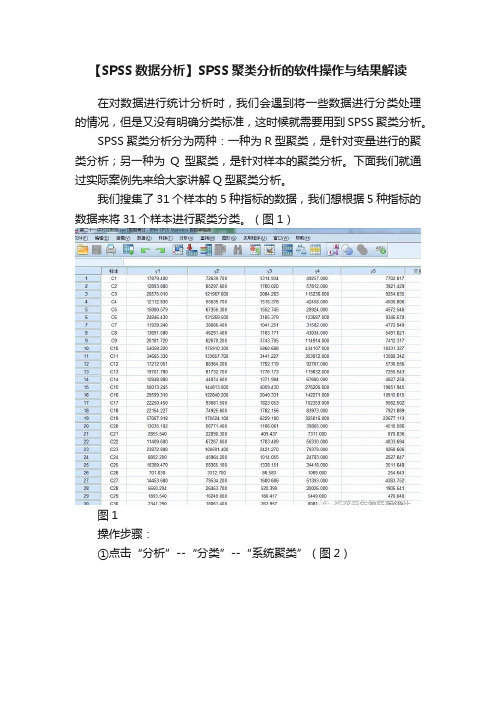
我们搜集了31个样本的5种指标的数据，我们想根据5种指标的数据来将31个样本进行聚类分类。

（图1）
图1
操作步骤：
①点击“分析”--“分类”--“系统聚类”（图2）
图2
③将“样本”选入个案标注依据，将γ1-5选入变量，并勾选下方“个案”标签（图3）
图3
④点击右侧“统计”按钮，将解的范围设置为2-4，意思为分聚为2,3,4类，这里可根据自己分类需求设置（图4）
图4
⑤点击右侧“图”，勾选“谱系图”（图5），点击右侧“方法”，将聚类方法设置为“组间联接”，将区间设置为“平方欧氏距离”（图6）
图5
图6
⑥点击“保存”，将解的范围设置为2-4（图7）
图7
⑦分析结果
图8
由上图（图8）可以看出，第一列为31个样本聚为4类的结果，第二列为31个样本聚为3类的结果，第三列为31个样本聚为2类的结果。

至于冰柱图和谱系图都是用图形化来进一步表达这个些结果，这里就不再赘述，想学习的朋友可以关注我们公众号进行深入学习。

以上就是今天所讲解的SPSS聚类分析的软件操作与分析结果详解，回顾一下重点，Q型聚类是根据变量数据针对样本进行的聚类。

然而还有R型聚类我们将在下一期中进行详细的讲解和分析。

敬请大家的关注！。

第九章SPSS的聚类分析

第九章SPSS的聚类分析1.引言聚类分析是一种数据分析方法，用于将相似的对象划分到同一组中，同时将不相似的对象划分到不同的组中。

SPSS是一种常用的统计软件，提供了聚类分析的功能。

本章将介绍SPSS中的聚类分析方法及其应用。

2.数据准备在进行聚类分析之前，需要准备好待分析的数据。

数据应该是定量变量或者定性变量，可以包含多个变量。

如果存在缺失值，需要处理之后才能进行聚类分析。

3.SPSS中的聚类分析方法在SPSS中，聚类分析方法有两种：基于距离的聚类和基于密度的聚类。

基于距离的聚类方法将对象划分到不同的组中，使得组内的对象之间的距离最小，组间的对象之间的距离最大。

常见的基于距离的聚类方法包括单链接聚类、完全链接聚类和平均链接聚类。

基于密度的聚类方法则通过考虑对象周围的密度来划分对象所属的组。

在SPSS中，可以使用层次聚类和K均值聚类这两种方法进行聚类分析。

3.1层次聚类层次聚类又称为分级聚类，它将对象分为一个个的层级，直到每个对象都成为一个单独的组为止。

层次聚类分为两种方法：凝聚层次聚类和分化层次聚类。

凝聚层次聚类是从每个对象作为一个单独的组开始，然后根据对象之间的距离逐渐合并组，直到所有的对象都合并到一个组为止。

凝聚层次聚类的最终结果是一个层级的分组结构，可以根据需要确定分组的层数。

分化层次聚类是从所有的对象开始，然后根据对象之间的距离逐渐分离成不同的组，直到每个对象都成为一个单独的组为止。

在SPSS中，可以使用层次聚类方法进行聚类分析。

通过选择合适的距离度量和链接方法，可以得到不同的聚类结果。

3.2K均值聚类K均值聚类是一种基于距离的聚类方法，通过计算对象之间的距离，将对象分为K个组。

K均值聚类的基本思想是：首先随机选择K个对象作为初始的聚类中心，然后将每个对象分配到离它最近的聚类中心，重新计算聚类中心的位置，直到对象不再发生变化为止。

K均值聚类的结果是每个对象所属的聚类，以及聚类的中心。

在SPSS中，可以使用K均值聚类方法进行聚类分析。

SPSS聚类分析具体操作步骤spss如何聚类

算法步骤：初始化聚类中心、分配数据点到最近的聚类中心、重新计算聚类中心、迭代直到聚类中心不再变化
适用场景：探索性数据分析、市场细分、异常值检测等
注意事项：选择合适的聚类数目、处理空值和异常值、考虑数据的尺度问题
定义：根据数据点间的距离或相似性，将数据点分为多个类别的过程常用方法：层次聚类、K-均值聚类、DBSCAN聚类等适用场景：适用于探索性数据分析，发现数据中的模式和结构注意事项：选择合适的距离度量方法、确定合适的类别数目等
常见的聚类分析方法包括层次聚类、Kmeans聚类、DBSCAN聚类等。
聚类分析基于数据的相似性或距离度量，将相似的数据点归为一类，使得同一类中的数据点尽可能相似，不同类之间的数据点尽可能不同。
聚类分析广泛应用于数据挖掘、市场细分、模式识别等领域。
K-means聚类：将数据划分为K个簇，使得每个数据点到所在簇中心的距离之和最小
聚类结果的可视化：通过图表展示聚类结果聚类质量的评估：使用适当的指标评估聚类效果的好坏聚类结果的解释：根据实际需求和背景知识，对聚类结果进行合理的解释和解读聚类结果的应用：探讨聚类结果在各个领域的应用场景和价值
SPSS聚类分析常用方法
定义：将数据集划分为K个聚类，使得每个数据点属于最近的聚类中心
聚类结果展示：通过图表或表格展示聚类结果，包括各类别的样本数和占比
聚类质量评估：采用适当的指标评估聚类效果，如轮廓系数、Davies-Bouldin指数等
聚类结果解读：根据业务背景和数据特征，解释各类别的含义和特征聚类结果应用：说明聚类分析在具体场景中的应用，如市场细分、客户分类等
SPSS聚类分析注意事项
确定聚类变量：选择与聚类目标相关的变量，确保变量间无高度相关性。

SPSS两步聚类的设置_SPSS 统计分析从入门到精通_[共3页]

分类分析第 12 章（2）AIC准则和BIC准则。

在两步聚类的第二步中用到的两个确定聚类个数的判断依据。

（3）调谐算法（Tuning the Algorithm）。

两步聚类过程既可以自动聚类，也可以人为控制聚类过程。

在人为控制时，需要用户指定参数，在这里称作调谐（tuning），参数指定了，聚类特征树的规模就基本确定了。

（4）噪声处理（Noise Handling）。

构建CFT树时，如果指定了聚类个数等参数，而观测量又很多的话，有可能发生CFT树长满而不能再长的情况。

那些没有长在树上的观测量就称为噪声，可以调整参数重新计算以让CFT树容纳更多的观测；也可以直接把它们归入某个类中或者直接丢掉。

（5）局外者（Outlier）。

对CFT树进行噪声处理后，被丢掉的观测量称之为局外者，它们单独构成一类，但不计入聚类结果的类别个数中。

12.4.2 问题描述和数据准备本节仍使用关于汽车制造商的例子（第12.3节系统聚类曾使用），目的是通过对多种车型在售价、物理特性等数据的聚类分析对这些车型进行归类和描述。

在系统聚类中，选取了对车种和销量进行特定限制的车型进行分析；在两步聚类中，将对所有数据进行分析。

案例数据均摘录自SPSS自带的演示文件“~\Samples\English\car_sales.sav”，所用数据文件来自随盘文件“Chapter 12\汽车销售初始数据.sav”，数据格式如图12-22所示。

图12-22 汽车销售初始数据的格式12.4.3 SPSS两步聚类的设置依次单击菜单“分析→分类→两步聚类…”打开两步聚类分析过程的主设置面板，如图12-23所示，在此指定分析变量、聚类个数等内容。

1．主面板的设置在左侧的变量列表中选中从“价格”到“用油效率”的9个变量，单击从上至下第二个按钮，将其指定为待分析的连续变量；在左侧的变量列表中单击选中“车种”变量，单击从上至下第一个按钮，将其指定为待分析的分类变量。

第九章SPSS的聚类分析

第九章SPSS的聚类分析聚类分析是一种将相似个体或对象归类到同一组中的统计方法，它通过测量个体或对象之间的相似性或距离来确定聚类的结构。

聚类分析在许多领域中都有广泛的应用，如市场分析、社会科学研究和生物学等。

在SPSS中进行聚类分析可以帮助研究人员和分析师更好地理解数据的结构和模式。

SPSS的聚类分析功能位于“分析”菜单下的“分类”子菜单中。

在打开聚类分析对话框后，用户需要选择聚类变量，并可以设置合适的聚类方法和距离度量。

可以使用的聚类方法包括层次聚类和K均值聚类，常用的距离度量有欧氏距离和曼哈顿距离等。

此外，用户还可以选择是否进行标准化处理和设置聚类数目等。

在进行聚类分析之前，用户需要对变量进行适当的数据准备工作，如缺失值处理、异常值处理和变量转换等。

这些数据准备步骤可以在“转换”菜单中的相应功能中完成。

对于聚类分析的结果，SPSS提供了多种显示和解释的方法。

在聚类过程完成后，SPSS会自动生成聚类结果的总结报告，该报告包含了关于聚类数目和每个聚类的统计信息。

用户可以通过“聚类概括”选项卡中的预览按钮查看聚类结果的总结报告。

此外，用户还可以通过“数量聚类输出”选项卡中的可视化按钮来生成聚类结果的可视化图形，如散点图和聚类树等。

在解释聚类分析的结果时，用户应该关注聚类数目和每个聚类的特征。

聚类数目可以根据数据的结构和目标进行选择，一般来说，聚类数目越多，聚类结果更详细，但也更复杂。

每个聚类的特征指的是在该聚类中具有相似特征的个体或对象。

用户可以通过查看每个聚类的平均值和标准差来得到关于每个聚类的特征。

总之，在SPSS中进行聚类分析可以帮助研究人员和分析师更好地理解数据的结构和模式。

通过选择合适的聚类变量、聚类方法和距离度量，以及适当的数据准备和结果解释，用户可以得到有关数据聚类结构的有用信息。

SPSSAU聚类分析步骤说明

聚类分析聚类分析：聚类分析是通过数据建模简化数据的一种方法。

“物以类聚，人以群分”正是对聚类分析最好的诠释。

一、聚类分析可以分为：对样本进行聚类分析（Q型聚类）,此类聚类的代表是K-means聚类方法；对变量（标题）进行聚类分析（R型聚类），此类聚类的代表是分层聚类。

常见为样本聚类，比如有500个人，这500个人可以聚成几个类别。

下面具体阐述对样本进行聚类分析的方法说明（分层聚类将在之后的文章中介绍）：聚类分析（Q型聚类）用于将样本进行分类处理，通常是以定量数据作为分类标准。

如果是按样本聚类，则使用SPSSAU的进阶方法模块中的“聚类分析”功能，其会自动识别出应该使用K-means聚类算法还是K-prototype聚类算法。

二、Q型聚类分析的优点：1、可以综合利用多个变量的信息对样本进行分类；2、分类结果是直观的，聚类谱系图非常清楚地表现其数值分类结果；3、聚类分析所得到的结果比传统分类方法更细致、全面、合理。

三、分析思路以下分析思路为对样本进行聚类分析（1）指标归类当研究人员并不完全确定题项应该分为多少个变量，或者研究人员对变量与题项的对应关系并没有充分把握时，可以使用探索性因子分析将各量表题项提取为多个因子（变量），利用提取得到的因子进行后续的聚类分析。

特别提示：分析角度上，通过探索性因子分析，将各量表题项提取为多个因子，提取出的因子可以在后续进行聚类分析。

比如：可先讲20个题做因子分析，并且得到因子得分。

将因子得分在进一步进行聚类分析。

最终聚类得到几个类别群体。

再去对比几个类别群体的差异等。

（2）聚类分析第一步:进行聚类分析设置如果使用探索性因子分析出来的因子进行聚类分析，当提取出五个因子时，应该首先计算此五个因子对应题项的平均分，分别使用平均得分代表此五个因子(比如因子1对应三个题项，则计算此三个题项的平均值去代表因子1)，利用计算完成平均得分后得到的因子进行聚类分析。

第二步:结合不同聚类类别人群特征进行类别命名聚类分析完成后，每个类别的样本应该如何称呼，或者每个类别样本的名字是什么，软件并不能进行判断。

IBM SPSS MODELER 实验一、聚类分析

IBM SPSS Modeler 实验一、聚类分析在数据挖掘中，聚类分析关注的内容是一些相似的对象按照不同种类的度量构造成的群体。

聚类分析的目标就是在相似的基础上对数据进行分类。

IBM SPSS Modeler提供了多种聚类分析模型，其中主要包括两种聚类分析，K-Mean 聚类分析和Kohonen聚类分析，下面对各种聚类分析实验步骤进行详解。

1、K-Means聚类分析实验首先进行K-Means聚类实验。

（1）启动SPSS Modeler 14.2。

选择“开始”→“程序”→“IBM SPSS Modeler 14.2”→“IBM SPSS Modeler 14.2”，即可启动SPSS Modeler程序，如图1所示。

图1 启动SPSS Modeler程序（2）打开数据文件。

首先选择窗口底部节点选项板中的“源”选项卡，再点击“可变文件”节点，单击工作区的合适位置，即可将“可变文件”的源添加到流中，如图2所示。

右键单击工作区的“可变文件”，选择“编辑”，打开如图3的编辑窗口，其中有许多选项可供选择，此处均选择默认设定。

点击“文件”右侧的“”按钮，弹出文件选择对话框，选择安装路径下“Demos”文件夹中的“DRUG1n”文件，点击“打开”，如图4所示。

单击“应用”，并点击“确定”按钮关闭编辑窗口。

图2 工作区中的“可变文件”节点图3 “可变文件”节点编辑窗口图4 文件选择对话框图5 工作区中的“表”节点（3）借助“表（Table）”节点查看数据。

选中工作区的“DRUG1n”节点，并双击“输出”选项卡中的“表”节点，则“表”节点出现在工作区中，如图5所示。

运行“表”节点（Ctrl+E或者右键运行），可以看到图6中有关病人用药的数据记录。

该数据包含7个字段（序列、年龄(Age)、性别(Sex)、血压(BP)、胆固醇含量(Cholesterol)、钠含量(Na)、钾含量(K)、药类含量(Drug)），共200条信息记录。

SPSS聚类和判别分析

在层次聚类中，度量数据之间的亲疏程度是极为关键的。在衡量样本与样本之间的距离时，一般使用的距离有Eulcidean Distance、Squared Euclidean Distance、切比雪夫距离、Block距离、明可斯基距离（Minkowshi ）、夹角余弦（Cosine）等。
1 8.193 3.909 1.303 .434 .145 .048 .016 .005 .002 .001
聚类中心内的更改
2
3
9.889
13.472
7.631
4.701
1.526
.672
.305
.096
.061
.014
.012
.002
.002
.000
.000
3.996E-5
9.768E-5
5.709E-6
➢ 变量间的关系度量模型与样本间相类似，只不过一个用矩阵的行进行计算，另一个用矩阵的列进行计算。
6
SPSS 19(中文版)统计分析实用教程
主要内容
9.1 聚类与判别分析概述 9.2 二阶聚类 9.3 K-均值聚类 9.4 系统聚类 9.5 判别分析
电子工业出版社
7
SPSS 19(中文版)统计分析实用教程
聚类 1 2 3
有效缺失
2.000 4.000 6.000 12.000
.000
可看出第1，2，3类中分别含有2，4，6个样本
21
SPSS 19(中文版)统计分析实用教程
9.3 K-均值聚类
➢分类保存情况
电子工业出版社
查看数据文件，可看到多出两个变量，分别表示每个个案的具体分类归属和与类中心的距离。
SPSS 19(中文版)统计分析实用教程

使用SPSS做两步聚类分析

SPSS T WO S TEP C LUSTER–A F IRST E VALUATION∗Johann Bacher†,Knut Wenzig‡,Melanie V ogler§Universit¨a t Erlangen-N¨u rnbergSPSS11.5and later releases offer a two step clustering method.According to the authors’knowledge the procedure has not been used in the social sciences until now.This situation is surprising:The widely used clustering algorithms,k-means clustering and agglomerative hierarchical techniques,suffer from well known problems,whereas SPSS TwoStep clustering promises to solve at least some of these problems.In particular,mixed type attributes can be handled and the number of clusters is automatically determined.These properties are promising. Therefore,SPSS TwoStep clustering is evaluated in this paper by a simulation study. Summarizing the results of the simulations,SPSS TwoStep performs well if all variables are continuous.The results are less satisfactory,if the variables are of mixed type.One reason for this unsatisfactoryﬁnding is the fact that differences in categorical variables are given a higher weight than differences in continuous variables.Different combinations of the categor-ical variables can dominate the results.In addition,SPSS TwoStep clustering is not able to detect correctly models with no cluster tent class models show a better perfor-mance.They are able to detect models with no underlying cluster structure,they result more frequently in correct decisions and in less unbiased estimators.Key words:SPSS TwoStep clustering,mixed type attributes,model based clustering,latent class models 1INTRODUCTIONSPSS11.5and later releases offer a two step clustering method(SPSS2001,2004).According to the authors’knowledge the procedure has not been used in the social sciences until now. This situation is surprising:The widely used clustering algorithms,k-means clustering and agglomerative hierarchical techniques,suffer from well known problems(for instance,Bacher 2000:223;Everitt et al.2001:94-96;Huang1998:288),whereas SPSS TwoStep clustering promises to solve at least some of these problems.In particular,mixed type attributes can be handled and the number of clusters is automatically determined.These properties are promising.∗AUTHORS’NOTE:The study was supported by the Staedtler Stiftung N¨u rnberg(Project:”Was leisten Clus-teranalyseprogramme?Ein systematischer Vergleich von Programmen zur Clusteranalyse“).We would like tothank SPSS Inc.(Technical Support),Jeroen Vermunt and David Wishart for invaluable comments on an earlierdraft of the paper and Bettina Lampmann-Ende for her help with the English version.†bacher@wiso.uni-erlangen.de‡knut@wenzig.de§vogler.m@gmx.deTherefore,SPSS TwoStep clustering will be evaluated in this paper.The following questionswill be analyzed:1.How is the problem of commensurability(different scale units,different measurementlevels)solved?2.Which assumptions are made for models with mixed type attributes?3.How well does SPSS TwoStep–especially the automatic detection of the number ofclusters–perform in the case of continuous variables?4.How well does SPSS TwoStep–especially the automatic detection of the number ofclusters–perform in the case of variables with different measurement levels(mixed typeattributes)?The model of SPSS TwoStep clustering will be described in the next section.The evaluationwill be done in section3.Section4will give concluding remarks.2SPSS TWOSTEP CLUSva.21249.471(TW)10.0583(O)0.3.STEPTwotep cluste e11Phrelioe li-310.061a6421995c01737(n=)0.2e0078–451.582(v)24.9835(a.)24423)0.132331)-0.160512(t).552(v)24.9835(a5.97593-0.132(;)Tj0.582 clektva725.986l ne(e)-0.161737(d)-240512((b)0.131718d70.132331(7(d)-240512((b)0.131718td)5533 12((b)0.13whereξi=−n i p∑j=112log(ˆσ2i j+ˆσ2j)−q∑j=1m j∑l=1ˆπi jl log(ˆπi jl) (2)ξs=−n s p∑j=112log(ˆσ2s j+ˆσ2j)−q∑j=1m j∑l=1ˆπs jl log(ˆπs jl) (3)ξ i,s =−n i,s p∑j=112log(ˆσ2 i,s j+ˆσ2j)−q∑j=1m j∑l=1ˆπ i,s jl log(ˆπ i,s jl) (4)ξv can be interpreted as a kind of dispersion(variance)within cluster v(v=i,s, i,s ).ξvconsists of two parts.Theﬁrst part−n v∑12log(ˆσ2v j+ˆσ2j)measures the dispersion of the con-tinuous variables x j within cluster v.If onlyˆσ2v j would be used,d(i,s)would be exactly the decrease in the log-likelihood function after merging cluster i and s.The termˆσ2j is added to avoid the degenerating situation forˆσ2v j=0.The entropy−n v∑q j=1∑m j l=1ˆπv jl log(ˆπv jl)is used in the second part as a measure of dispersion for the categorical variables.Similar to agglomerative hierarchical clustering,those clusters with the smallest distance d(i,s)are merged in each step.The log-likelihood function for the step with k clusters is com-puted asl k=k∑v=1ξv.(5)The function l k is not the exact log-likelihood function(see above).The function can be interpreted as dispersion within clusters.If only categorical variables are used,l k is the entropy within k clusters.Number of clusters.The number of clusters can be automatically determined.A two phase estimator is used.Akaike’s Information CriterionAIC k=−2l k+2r k(6) where r k is the number of independent parameters or Bayesian Information CriterionBIC k=−2l k+r k log n(7) is computed in theﬁrst phase.BIC k or AIC k result in a good initial estimate of the maximum number of clusters(Chiu et al.2001:266).The maximum number of clusters is set equal to number of clusters where the ratio BIC k/BIC1is smaller than c1(currently c1=0.04)1for the ﬁrst time(personal information of SPSS Technical Support).In table1this is the case for eleven clusters.The second phase uses the ratio change R(k)in distance for k clusters,deﬁned asR(k)=d k−1/d k,(8) 1The value is based on simulation studies of the authors of SPSS TwoStep Clustering.(personal information of SPSS Technical Support,2004-05-24)where d k−1is the distance if k clusters are merged to k−1clusters.The distance d k is deﬁned similarly.2The number of clusters is obtained for the solution where a big jump of the ratio change occurs.3The ratio change is computed asR(k1)/R(k2)(11) for the two largest values of R(k)(k=1,2,...,k max;k max obtained from theﬁrst step).If the ratio change is larger than the threshold value c2(currently c2=1.154)the number of clusters is set equal to k1,otherwise the number of clusters is set equal to the solution with max(k1,k2). In table1,the two largest values of R(k)are reported for three clusters(R(3)=2.129;largest value)and for eight clusters(R(8)=1.952).The ratio is1.091and smaller than the threshold value of1.15.Hence the maximum of3resp.8is selected as the best solution.Cluster membership assignment.Each object is assigned deterministically to the closest clus-ter according to the distance measure used toﬁnd the clusters.The deterministic assignment may result in biased estimates of the cluster proﬁles if the clusters overlap(Bacher1996:311–314,Bacher2000).Modiﬁcation.The procedure allows to deﬁne an outlier treatment.The user must specify a value for the fraction of noise,e.g.5(=5%).A leaf(pre-cluster)is considered as a potential outlier cluster if the number of cases is less than the deﬁned fraction of the maximum cluster size.Outliers are ignored in the second step.pared to k-means algorithm(QUICK CLUSTER)or agglomerative hierarchical techniques(CLUSTER),SPSS has improved the output signiﬁcantly.An additional modul allows to statistically test the inﬂuence of variables on the classiﬁcation and to compute conﬁdence levels.3EV ALUATION3.1CommensurabilityClustering techniques(k-means-clustering,hierarchical techniques etc.)require commensu-rable variables(for instance,Fox1982).This implies interval or ratio scaled variables with equal scale units.In the case of different scale units,the variables are usually standardized by the range(normalized to the range[0,1],range weighted)or z-transformed to have zero mean and unit standard deviation(autoscaling,standard scoring,standard deviation weights).If the variables have different measurement levels,either a general distance measure(like Gower’s general similarity measure;Gower1971)may be used or the nominal(and ordinal)variables may be transformed to dummies and treated as quantitative5(Bender et al.2001;Wishart2003). 2The distances d k can be computed from the output in the following way:d k=l k−1−l k(9)l v=(r v log n−BIC v)/2or l v=(2r v−AIC v)/2for v=k,k−1(10) However,using BIC or AIC results in different solutions.3The exact decision rules are described vaguely in the relevant literature and the software documentation(SPSS 2001;Chiu et al.2001).Therefore,we report the exact decision rule based on personal information of SPSS Technical Support.A documentation in the output,like“solution x was selected because...”,would be helpfull for the user.4Like c1,c2is based on simulation studies of the authors of SPSS TwoStep Clustering.(personal information of SPSS Technical Support,2004-05-24)5The term“quantitative”will be used for interval or ratio scaled variables.Table1.SPSS TwoStep Auto Clustering ResultsSchwarz’s Bayesian Criterion (BIC)BICChange aRatio ofBICChanges bRatio ofDistanceMeasures c181490.274256586.953−24903.3201.0001.467339624.406−16962.547.6812.129←Maximum ratio of distance 431686.789−7937.617.3191.343525792.248−5894.541.2371.010619955.794−5836.454.2341.745716636.600−3319.194.1331.177813825.500−2811.100.1131.952←SPSS decision(see text) 912414.105−1411.396.0571.0141011022.935−1391.169.0561.036max.number119682.323−1340.612.0541.755←of clusters128943.800−738.523.0301.005in phase1a The changes result from the previous number of clusters in the table.b The ratio of changes is with respect to the change at the two clusters.c The ratio of distance measures is based on the current number of clusters in relation to the previous number of clusters.Treshold values of Fraley&Raftery(1998:582):BIC Change less than2=weak evidence;BIC Change between two and six=positive evidence;BIC Change between six and ten=strong evidence;BIC Change greater than ten =strong evidence.Note:SPSS TwoStep computes either BIC or AIC.If both measures are needed the procedure must be run two times.The ratio of distance measure is equal for BIC and AIC.SPSS TwoStep clustering offers the possibility to handle continuous and categorical variables. Hence,SPSS TwoStep cluster model only provides a solution for a special case of variables of mixed type.Quantitative variables with different scale units and nominal scaled variables may be simultaneously analyzed.The user must decide to handle ordinal variables either as continuous or as categorical if they are present.Continuous variables are z-standardized by default in order to make them commensurable. This speciﬁcation is not the consequence of the statistical model used in SPSS TwoStep.Hence, other procedure can be used too.Z-standardization may be appropriate in some applications, in others not(Bacher1996:173–198;Everitt1981:10;Everitt et al.2001:51–52).If random errors are the reasons of larger variances,z-standardization has a positive effect:Variables with large proportions of random errors are given lower weights.However,if differences between clusters result in larger variances,z-standardization has a negative effect:Variables that separate the clusters well are given lower weights.In empirical studies the reasons for high variances are unknown.Probably,both reasons apply so that both effects cancel out.Simulation studies suggest,that z-standardization is ineffective(for a summary of simulation results;see Everitt et al.2001:51).Better results are reported for standardization to unit range(ibidem).However, standardization to unit range is problematic for mixed type attributes(see below).In the case of different measurement levels,the distance measures for the different kinds of variables must be normalized in order to make them commensurable.The log-likelihood dis-tance uses the following normalization.If two objects i and s differ only in one categorical variable and are merged to one cluster i,s ,the log-likelihood distance is0.602.This distancecorresponds to a difference of2.45scale units(=standard deviation)if two objects differ in one standardized continuous variable.6Hence,a difference in one categorical variable is equal to a difference of2.45scale units in one standardized continuous variable.This normalization may favor categorical variables to deﬁne clusters(see below).This effect would even be stronger for standardization by range:The maximum difference between two objects that differ only in one continuous variable is0.1767,whereas the maximum difference between two objects that differ only in one categorical variable is0.602.Hence,a difference in one categorical variable is given a three times higher weight than the maximum difference in continuous variables that are standardized by range.This disadvantage seems to be more serious than the above men-tioned better perfomance of standardization by range.Therefore,z-standardization seems an acceptable approach.Table2compares SPSS TwoStep clustering with other clustering procedures.K-means im-plementation and latent class models tent probabilistic clustering models8are used. Compared to k-means-implementations,SPSS TwoStep allows to handle continuous and cat-egorical variables.9Compared to latent class models,SPSS TwoStep performs worse.Both latent models are able to handle all kind of measurement levels.Different scale units cause no problems,they are model based transformed.3.2Automatic Determination Of The Number Of ClustersChiu et al.(2001)report excellent results for the proposed algorithm to determine the number of clusters automatically.For about98%of the generated data sets(more than thousands),SPSS TwoStep clustering was able toﬁnd the correct number of clusters.For the rest the clusters were indistinguishable due to much overlap.Data sets with overlapping clusters are characteristic for the social sciences.Therefore,we analyzed artiﬁcial datasets with overlap.Five different cluster models were studied(see table3). 6According to formula1,the log-likelihood distance d(i,s)is equal tod(i,s)=0+0− −2 0quantitative var.−(0.5log(0.5)+0.5log(0.5))=0.6021,(12)if two objects i and s that differ only in one nominal variable are combinded.(ξi(formula2)andξs(formula3) are zero,because“clusters”i and s contain only one object.)This corresponds to a difference of+2 12log ˆσ2 i,s j+ˆσ2j =0.6021⇔100.6021=4=ˆσ2 i,s j+ˆσ2j 1⇔3=(x i j−x s j)2/2ˆσ2 i,s j⇔±2.45=x i j−x s j,(13)if n−1is used to estimate the variances.If n is used,x i j−x s j=±1.73.The different weighting of differences in categorical and continuous variables can be illustrated by the following example,too:If a standard normal distribution N(0,1)is dichotomized at point0,the average distance between two randomly selected objects is0.24if the variable is treated as continuous.If the variable is treated as categorical,the average distance between two randomly selected objects is0.30and1.25times higher than the value if the variable is speciﬁed as continuous.Intuitively,one would expect that both values are equal.7The value of d(i,s)is equal to+2(12log(ˆσ2i,s +ˆσ2j))=log(+0.5+1)=0.1761,if we setˆσ2j=1in order toguarantee positive values for d(i,s).If n is used to estimate the variances,d(i,s)is equal0.301.8Bacher(2000)proves that latent class models can be interpreted as probabilistic clustering models.In contrast to deterministic clustering techniques,cases are assigned to the cluster probabilistically.9Note:This comparision refers only to the solutions of the problem of commensurabilty for the different k-means implementations.Hence,this comparisions is not a benchmark test of k-means implementations or statistical clustering software.3EV ALUATION Table 2.Solutions Of Incommensurabilty In Different Software Packagesk-means-clustering latent class modelsSPSS Quick Cluster a ALMO Prog37b SAS c CLUSTAN k-means dSPSS TwoStep a LatentGold e ALMO Prog37bdifferent scale units no,syntax lan-guage can be used to standardize and weight variables,variables may be standardized with the procedure DESCRIPTIVESz-standardization resp.different methods of weighting can be used;syntax language can beused,tooz-standardization recommended,SAS procedure STANDARD is availablez-standardization,standardization to (unit)range,weighting possible z-standardization not necessary,commensurability is solved model based not necessary,commensurabilityis solved modelbaseddifferent measurement levels no,syntax can be used to solve the problem (see Bacher 2002;Bender et al.2001)nominal (including binary)and quantitative are allowed;ordinal variables are treated as interval no,similar to SPSS syntax can be used nominal (including binary),ordinal and quantitative nominal and quantitative variables only,user must decide how to handle ordinal variablesnominal (including binary),ordinal and quantitative,different model based procedures nominal (including binary),ordinal and quantitative,different modelbased proceduressyntax and other procedures to solve the problem of incommensura-bilityyes yes yes Auto Script allows a script ﬁle to be run (since Version 6.03)yes no,except some basic transforma-tionsyesa SPSS Version 11.5was used.Further information is available under http//:b Version 7.1.ALMO is a standard statistical package developed by Kurt Holm (http://www.almo-statistik.de ).The cluster program was developed by the author of this paper.Prog37contains models for k-means-clustering using a general variance formula and models for probabilistic clustering.The probabilistic clustering model is described in Bacher (2000).It allows to handle variables with mixed measurement levels.c The SAS OnlineDoc (SAS 2002)has been consulted,online available under /sasdoc/d ClustanGraphics is perhaps the best known stand alone clustering software und has been developed by David Wishart.ClustanGraphics contains a convincing dendrogramme technique and new develepments like focal point clustering,bootstrap validation and techniques for medoids (exemplars).FocalPoint uses different starting values to ﬁnd the best solution.Procedures to solve the problem of incommensurability are described in (Wishart 2003)and are available in version 6.06(personal information of David Wishart).Further information is available under .e Version 2.0was tent GOLD was developed by Jeroen K.Vermut and Jay Magidson.Version 3.0is available since the beginning of 2003.The default number of start sets as well as the default number of iterations per set.Version 4.0will come up after this summer and will contain new features.It will allow new scale types,namely “binomial count”,“truncated Poisson”,“truncated binomial count”,“truncated normal”and “censored normal”.Model validation will be improved by a bootstrap technique for the -2LL value (personal information of Jeroen Vermunt,2004-05-24).Information is available under 73EV ALUATIONOne model consists of one cluster.Two models consist of two clusters with different overlap. The fourth model consists of three clusters and theﬁfth model consists ofﬁve clusters.Two sets of variables were deﬁned for each model:one data set with three independent variables and one with six independent variables.A standard normal distribution was assumed for all variables.Two(resp.four)of the variables were categorized for the analysis.A category value of0was assigned if the values of the variable were less than or equal to−1;if the values were greater than−1and less than+1,a category value of1was assigned;and if the value was greater than or equal to+1,a category value of2was assigned.One of the two(resp.two of the four)variables were treated as nominal variables.The other categorical variable(s)were treated as ordinal variable(s).In order to test the effect of categorization and the performance of SPSS TwoStep for mixed type attributes the analysis was repeated with the original(uncategorized) variables.For purpose of illustrations,the quantitative variables can be interpreted as income(e.g.per-sonal income in the experiments with three variables,income of father and mother in the case of six variables to analyse the social status of children);the ordinal variables can be interpreted as education(e.g.personal education cation of father and mother)and the nominal variables can be interpreted as occupation(e.g.personal occupation resp.occupation of father and mother).The clusters represent social classes.The model with one cluster represents a so-ciety with no class structure.The model with two clusters corresponds to a two class structure (lower class and upper class are distinguishable),the model with three clusters represents a three class structure(lower class,middle class and upper class can be differentiated).The model with ﬁve clusters corresponds to aﬁve class structure.Two of theﬁve clusters have an inconsistent pattern.On the average,persons of cluster4have a high income,but a middle education(and occupation).They may be labeled the class of self-made man.In contrast,persons of cluster5 on the average have a middle income,but a high education(and occupation).This class may be labeled as the class of intellectuals.The other clusters correspond to upper class,middle class and lower class.For each model six artiﬁcial data sets with20,000cases were generated.In order to test the inﬂuence of sample size,we analyzed the total sample of20,000cases and subsamples with 10,000,5,000,2,000,1,000and500cases.In total,900data sets were generated.The results are summarized in table4.10Continuous resp.quantitative variables only.SPSS TwoStep is able to detect the correct number of clusters for the models with two and three classes(models M2a,M2b and M3). Sample size has no effect for those conﬁgurations.Some problems occur for the model with three clusters,if only three variables are used.The procedure selects sometimes two or four clusters.However,these defects are not severe(4of36).In contrast to these postive results,the model withﬁve clusters(M5)results in wrong deci-sions for the number of clusters in all experiments with20,000cases.SPSS TwoStep is not able toﬁnd the two small inconsistent clusters that were added to the three class structure.If three variables are analyzed the results are unstable.For instance,the procedure decides for six,four,ﬁve or three clusters if the sample size is10,000.In the case of six variables,the procedure results in three clusters.Model M0(no class structure)results in instable results,too.SPSS TwoStep is not able to analyze the question whether a cluster model underlies the data.10The simulation study was done with the German version of SPSS11.5.A replication with SPSS12.0(German version)and the English version of SPSS11.5reports differentﬁndings for some constellations.The differences are probably due to improvements of the algorithm(personal information of SPSS Technical Support,2004-05-24).3EV ALUATION Table 3.Analysed Artiﬁcial DatasetsCluster models Variablesthree resp.six random N(0,1)-variables x 1,x 2,...,x 6;three constellations of variables:SPSS TwoStep speciﬁcation:(1)all variables are quantitative ⇔mixed type attributes (2)ordinal variables are treated as quantitative ⇔(3)ordinal variables are treated as nominal ⇔(1)all variables are continuoustwo of them resp.four of them were categorized(2)one resp.two of them are treated as categorical(3)two resp.four of them are treated as categorical substantive interpretation (for purpose of illustration)one cluster (M0)cluster 1µ(x i )=0.00;i =1,2,3;n =20000resp.100%no class structure exists in the analyzed population two clusters (M2a)cluster 1cluster 2µ(x i )=−0.75;i =1,2,3;n =10000resp.50%µ(x i )=+0.75;i =1,2,3;n =10000resp.50%lower class upper class two classes are present,the classes are not well seperatedtwo clusters (M2b)cluster 1cluster 2µ(x i )=−1.50;i =1,2,3;n =10000resp.50%µ(x i )=+1.50;i =1,2,3;n =10000resp.50%lower class upper class two classes are present,the classes are well seperatedthree clusters (M3)cluster 1cluster 2cluster 3µ(x i )=−1.50;i =1,2,3;n =5000resp.25%µ(x i )=0.00;i =1,2,3;n =10000resp.50%µ(x i )=+1.50;i =1,2,3;n =5000resp.25%lower class middle classupper classthree not well seperated classesﬁve clusters (M5)cluster 1cluster 2cluster 3cluster 4cluster 5µ(x i )=−1.50;i =1,2,3;n =3000resp.15%µ(x i )=0.00;i =1,2,3;n =10000resp.50%µ(x i )=+1.50;i =1,2,3;n =3000resp.15%µ(x 1)=1.50;µ(x 2)=µ(x 3)=0.00;n =2000resp.10%µ(x 1)=0.00;µ(x 2)=µ(x 3)=1.50;n =2000resp.10%lower class middle class upper classselfmade manintellectualsthree not well seperated classes plus twoinconsistent classes µ(x i )=mean of a variable x i 93EV ALUATIONTable4.Number Of Clusters Computed By SPSS TwoStep(Results Of Simulation Studies)Cluster Model SampleSize nonly quantitativevariablesordinal var.treated ascategoricalordinal var.treated ascontinuous three var.six var.three var.six var.three var.six var.M020,0005,4,4,9,43,3,11,2,108,8,6,8,88,4,6,4,82,6,2,6,23,6,3,3,3 10,00010,2,6,9,56,8,7,7,56,3,3,8,85,4,4,6,46,2,2,2,23,6,3,3,35,0006,5,3,9,47,6,7,7,46,6,3,8,84,6,5,5,52,2,6,6,63,3,3,3,32,0004,5,7,4,116,5,5,4,33,8,3,3,84,4,4,8,62,2,6,6,63,3,3,3,31,0002,7,7,4,44,8,3,6,23,8,3,3,34,10,5,5,52,6,2,6,63,3,3,3,35003,3,6,2,24,4,4,5,63,3,6,3,85,4,5,5,42,2,2,6,63,3,3,3,3 M2a20,0002,2,2,2,22,2,2,2,210,7,7,10,72,2,2,2,23,3,3,3,38,8,8,8,8 10,0002,2,2,2,22,2,2,2,27,10,10,7,72,2,2,2,23,3,3,3,38,8,8,8,85,0002,2,2,2,22,2,2,2,27,7,7,10,72,2,2,2,23,3,3,3,38,8,8,8,82,0002,2,2,2,22,2,2,2,27,7,7,7,72,2,2,2,24,3,3,3,38,8,8,8,81,0002,2,2,2,22,2,2,2,27,7,7,7,72,2,3,2,23,3,3,3,38,8,8,8,85002,2,2,2,22,2,2,2,27,7,7,7,72,2,2,2,24,3,3,3,38,8,7,8,8 M2b20,0002,2,2,2,22,2,2,2,27,7,7,7,72,2,2,2,23,3,3,3,32,2,2,2,2 10,0002,2,2,2,22,2,2,2,27,7,7,7,72,2,2,2,23,3,3,3,32,2,2,2,25,0002,2,2,2,22,2,2,2,27,7,7,7,72,2,2,2,23,3,3,3,32,2,2,2,22,0002,2,2,2,22,2,2,2,27,7,7,7,72,2,2,2,23,3,3,3,32,2,2,2,21,0002,2,2,2,22,2,2,2,27,7,7,7,72,2,2,2,23,3,3,3,32,2,2,2,25002,2,2,2,22,2,2,2,27,7,7,7,72,2,2,2,23,3,3,3,32,2,2,2,2 M320,0003,3,3,2,33,3,3,3,310,7,7,7,73,3,2,3,33,3,3,3,37,7,7,7,7 10,0003,3,3,3,33,3,3,3,310,7,7,7,73,3,3,2,23,3,3,3,37,7,7,7,75,0003,3,4,3,33,3,3,3,310,7,7,10,102,2,3,2,23,3,3,3,37,7,7,7,72,0003,3,3,2,33,3,3,3,37,7,7,7,73,3,3,2,23,3,3,3,37,8,7,7,71,0003,3,3,3,33,3,3,3,37,7,7,7,73,3,2,3,23,3,3,3,37,7,7,7,75003,2,3,3,33,3,3,3,37,7,7,7,72,3,4,2,43,3,3,3,37,7,7,7,7 M520,0002,3,2,2,33,3,3,3,37,7,7,7,76,5,6,4,43,3,3,3,37,7,7,7,7 10,0006,4,4,5,33,3,3,3,37,7,7,7,76,5,6,3,33,3,3,3,37,7,7,7,75,0002,3,3,3,23,3,3,3,37,7,7,7,76,3,3,4,23,3,3,3,37,7,7,7,72,0003,3,6,2,43,3,3,3,37,7,7,7,76,7,2,6,63,3,3,3,37,7,7,7,71,0002,5,3,3,23,3,3,3,37,7,7,7,73,3,7,4,23,3,3,3,34,7,7,7,75003,2,4,2,43,3,3,3,37,7,7,7,76,2,3,6,33,3,3,3,34,4,7,7,7 A closer look to the distance ratio reveals that a small difference between the largest distance ratio and the second largest distance ratio occurs if SPSS TwoStep has problems to detect the correct number of clusters.The situation is similar to those reported in table1.Two or more cluster solutions have similar distance ratio around1.3to3.8.In contrast to this ambiguous situation,a large difference is computed in those cases where SPSS TwoStep computes the correct number of clusters:There is one large distance ratio(for the different models values greater than4.0,8.0,13.0,18.0or50.0)whereas the second largest value is small(maximum values of1.2to2.0).The results suggest that the ratio change R(k1)/R(k2)(formula11)should。

SPSS_Statistics_19_聚类分析

自然条件：降水、土地、日照、湿度等经济指标：收入水平、教育程度、医疗条件、基础设施等

平均的方法？

容易忽视相对重要程度的问题

要进行多元分类－聚类分析
3
1 聚类分析

聚类分析基本目标

一种探索性的数据分析技术
是根据数据本身结构特征对数据点进行分类的方法基本目标：在数据中寻找某种“自然的”分组结构
确定样品间相似的度量

距离度量相似性度量

确定样本点的聚类数量

实际应用中，一般推荐4-6类(5% < 细分群体占比 < 35%)

对聚类结果进行描述和解释

验证细分方案的可接受性描述各细分群体(交叉表分析) 市场定位(Positioning)
7
©确定目标消费群体 (Targeting) 2009 SPSS Inc.

24
3 K-均值聚类

非系统聚类

K均值聚类
优点

K均值聚类的速度快于系统聚类，是处理大型数据集聚类的常用方法
内存占用小

不足

只适用于连续型变量；只能对记录进行聚类，而不能对变量聚类；对初始聚类中心有一定的依赖性；由于要事先选定聚类数，所以要尝试多次，以找出最佳聚类
25
此外还有中间距离法（Median Clustering)、类内平均法(Within-Groups
Linkage)等
ቤተ መጻሕፍቲ ባይዱ12
2 系统聚类

系统聚类

优点

聚类变量可以是分类或连续型变量；既可以对变量聚类，也可以对数据点/记录聚类(市场细分一般都是对记录聚类)；一次运行即可得到完整的分类序列；

1、下载文档前请自行甄别文档内容的完整性，平台不提供额外的编辑、内容补充、找答案等附加服务。
2、"仅部分预览"的文档,不可在线预览部分如存在完整性等问题,可反馈申请退款(可完整预览的文档不适用该条件!)。
3、如文档侵犯您的权益，请联系客服反馈,我们会尽快为您处理(人工客服工作时间：9:00-18:30)。

・
２２・０
中国卫生统计２ｌ４月第２ｏＯ年７卷第２期
ＳＳＰＳ两阶聚类法如何自动确定聚类数
汪存友余嘉元・两阶聚类法（ｗｏｔｌｓｒＴＣ）ＳＳ１．ＴＳｅＣｕｔ，Ｓ是ＰＳ１５ｐｅ及之后版本中新增的一种聚类分析方法。与ＳＳＰＳ中提供的Ｋ—ｍｅｌ法和层次聚类分析法不同，法采ａｓｌ该有时会出现这样的情况，：着聚类个数的增加。即随ＢＣ会不断较小，此没有最小值。需要说明的是，Ｉ因ＴＣ还提供了与ＢＣ相近的统计指标ＡａｃＳＩｆｒＳＩｋｉ ’ ｏ－ｋｎｍａｏｒｒｎＡＣ，ＳＳｉｒｎＣｉｉ（Ｊ）但ＰＳ默认使用ＢＣｅｔｏＩ。
版本）带数据ｃｒｓｅ．ａ自ａａｓｓ＿ｌｙ为例阐述ＴＣ自动确定Ｓ聚类个数的规则。１操作演示．
打开ＳＳ１．，Ａａｚ－￣ｌｓｙ－ｗｏｔＰＳ３０按ｎｌｅ－ａｉ－ＴＳｐｙＣｓｆ＊ｅ
Ｃｕｔ顺序单击菜单项，ｌｓｒｅ进入两阶聚类分析主对话框。选择分类变量ｔｐ，人Ｃｔｒｉｌ中；择ｐｉ、ｙｅ送ａｇｏｃ框ｅａ选ｒｅｃ
表１自动聚类表
用对数极大似然估计值度量类间距离，并能根据施瓦兹贝叶斯准则（Ｉ）ＡａｅＢＣ或ｋｉ信息准则（Ｉ等指ｋＡＣ）标自动确定最佳聚类个数。ＴＣ的这一优点有利于Ｓ研究者在无任何先验知识时进行探索性聚类分析，因此该法在医学、融、金商业和心理学等领域有着广泛应
ｈｒｅｏｏｓｐｗｗｈｅｂｓｗｉｔｅｇｈ、ｕｂｗｇｅｌａ，ｄｈ、ｌｎｔｃｒｔ
—
ｆｅｃｕｌａｐ和
ｍｇ等９个连续变量，ｐ送人ＣｎｉｏｓｉｏｔｕｕｌｎＶａ—
ｏｆｒｎＣｔｉｉ — ｅ
ａｌｓ中，Ｏｕｕ对话框中勾选 “ｎｏｂｅ框在ｔｔｐＩｆ￣
类结果，ＳＴＣ将统计相应的联合对数极大似然估计值（ｏｎｅｔｔｎｏｇｍａｉｕｋｌｏｄＪＬＪｉｔｓｍａｏｆｏｘｍｍｌｅｈｏ，ＥＭＬ）ｉｉｌｉｉ，
大似然估计值的变化。与ｒＩＢＣ不同，该变化率是联合对数极大似然估计值在本次合并中发生的变化与前一
用。然而，内外鲜有学者论及ＴＣ究竟如何自动确国Ｓ定聚类个数 ¨ ；ＰＳ的技术文档虽然阐述了ＴＣＳＳＳ确定聚类个数的规则，其表述与ＳＳ但ＰＳ的实际输出结果却并不一致Ｊ。这导致人们对ＴＣ的自动确定Ｓ聚类数功能难以理解。为此，文以ＳＳ本ＰＳ软件（３０１．
２对自动聚类表的解读．ＳＳＰＳ输出的自动聚类表共有５列。
第一列为聚类个数。ＴＣ借鉴了凝聚型层次聚Ｓ类法的思路，：即系统默认最大聚类个数为ｌ，后逐５然个合并距离最小的两类，到为１个类。对于每种聚直
般认为，ＢＣ绝对值越大，ｄＩ聚类结果越理想。第四列为ＢＣ变化率，同样反映了合并前后两Ｉ它种聚类结果的ＢＣ变化情况。这里用ｍｌ（）示聚Ｉｃ．表，类个数为 ‘时的ＢＣ变化率，ＢＣ（）＝ｄＩ．，ＩｒＩ．，ＢＣ（０／ｄＩ２，：是由．类合并为Ｊ—ｌ时ＢＣ变化ＢＣ（）即它，类Ｉ与由２类合并为１时ＢＣ变化的比值。与ｄＩ类ＩＢＣ不同，ＢＣ取值在［一ｌ１之间，值在ＴＣ确定聚类ｒＩ，）该Ｓ个数时具有重要作用。第五列为最小距离变化率。由于ＴＣ采用对数Ｓ极大似然估计值度量类问距离，因此，最小距离变化本质上反映了距离最近的两类合并为一类时联合对数极
ｅｇｎｎｉｅ
—
＿
第三列为ＢＣ变化，Ｉ它反映了合并前后两种聚类结果的ＢＣ变化情况。这里，ＢＣ（）示聚类个Ｉ用Ｉ．表，数为．时的ＢＣ值，ｄＩ ‘ 表示聚类个数为时，Ｉ用ＢＣ（），
的ＢＣ变化，ｄＩ（）＝Ｉ．一１ＢＣ（）Ｉ则ＢＣ＇ＢＣ（，，）一ＩＪ。一
ｏ（ＩｒＩ ” 同时勾选 “ ｒａｌｓｒＩＩｅｐｎＡＣｏＣ），ＢＣｅｔｃｕｔｌｎｅｅＩｂபைடு நூலகம்ｅ
ｖｒｂ ” ａａｌ复选框，ｉｅ其他选项均为默认设置， “ Ｋ运点击Ｏ ” 行ＴＣ算法。表１Ｓ是聚类分析得到的自动聚类表，ＳＴＣ主要根据表１中的信息确定最佳聚类个数。
次合并时发生变化的比值，这里用ｒＭ（）Ｄ－表示聚类，个数为．时的最小距离变化率。一般认为，Ｄ（），ｒＭ＇，