First Order Stochastic Dominance in Truncated Log-Normal Distributions
金融时间序列分析英文试题(芝加哥大学) (1)
Graduate School of Business,University of ChicagoBusiness41202,Spring Quarter2008,Mr.Ruey S.TsaySolutions to MidtermProblem A:(30pts)Answer briefly the following questions.Each question has two points.1.Describe two methods for choosing a time series model.Answer:Any two of(a)Information criteria such as AIC or BIC,(b)Out-of-sample forecasts,and(c)ACF and PACF of the series.2.Describe two applications of volatility infinance.Answer:Any two of(a)derivative(option)pricing,(b)risk management,(c)portfolio selection or asset allocation.3.Give two applications of seasonal time series models infinance.Answer:(a)Earnings forecasts and(b)weather-related derivative pricing or risk man-agement.4.Describe two weaknesses of the ARCH models in modelling stock volatility.Answer:Any two of(a)symmetric response to past positive and negative shocks,(b)restrictive,(c)Not adaptive,and(d)provides no explanation about the source ofvolatility clustering.5.Give two empirical characteristics of daily stock returns.Answer:any two of(a)heavy tails,(b)non-Gaussian distribution,(c)volatility clus-tering.6.The daily simple returns of Stock A for the last week were0.02,0.01,-0.005,-0.01,and0.025,respectively.What is the weekly log return of the stock last week?What is theweekly simple return of the stock last week?Answer:Weekly log return is0.03938;weekly simple return is0.04017.7.Suppose the closing price of Stock B for the past three trading days were$100,$120,and$100,respectively.What is the arithmetic mean of the simple return of the stock for the past three days?What is the geometric average of the simple return of the stockfor the past three days? Answer:Arithmetic mean=12120−100100+100−120120=0.017.and the geometric mean is120×100−1=0.8.Consider the AR(1)model r t=0.02+0.8r t−1+a t,where the shock a t is normally distrib-uted with mean zero and variance1.What are the variance and lag-1autocorrelation function of r t?Answer:Var(r t)=11−0.82=2.78and the lag-1ACF is0.8.19.For problems6and7,suppose the daily return r t,in percentages,of Stock A followsthe model r t=1.0+a t+0.3a t−1,where a t=σt t withσ2t =1.0+0.4a2t−1and t beingstandard normal.What is the unconditional variance of a t?What is the variance of r t?Answer:Var(a t)=11−0.4=1.67.Var(r t)=(1+0.32)σ2a=1.82.10.Suppose that a n=3.0,what is the1-step ahead forecast for r n+1at the forecast originn?What is the1-step ahead volatility forecast of r t at the forecast origin n?Answer:r n(1)=1+0.3a n=1.9,andσ2n (1)=1+0.4a2n=4.6.11.Consider the simple AR(1)model r t=100+0.8r t−1+a t,where a t is normally distributedwith mean zero and variance10.Is the r t series mean-reverting?If yes,what is the half-life of the series?Answer:Yes,r t series is mean-reverting.The half-life is ln(0.5)/ln(0.8)=3.11.12.Describe two test statistics for testing the ARCH effect of an asset return series.Writedown the associated null hypotheses.Answer:(a)The Ljung-Box statistic Q(m)of the squared shocks,i.e.a2t .The nullhypothesis is H o:ρ1=ρ2=···=ρm=0,whereρi is the lag-i ACF of a2t .(b)TheEngle F-test for the regression a2t =β0+β1a2t−1+···+βm a2t−m+e t.The null hypothesisis H o:β1=β2=···=βm=0.13.Consider the following two IGARCH(1,1)models for percentage log returns:Model A:σ2t =1.0+0.1a2t−1+0.9σ2t−1Model B:σ2t =0.1a2t−1+0.9σ2t−1.Suppose thatσ2100=20and a100=−2.0.What are the3-step ahead volatility forecastsfor Models A and B?Answer:For model A:3-step ahead volatility forecast isσ2100(3)=2+(1.0+0.1×(−2.0)2+0.9×20)=21.4.For model B,the3-step ahead volatility forecast isσ2100(3)=0.1(−2.0)2+0.9×20=18.4.14.Consider the following two models for the log price of an asset:Model A:p t=p t−1+a tModel B:p t=0.00001+p t−1+a twhere the shock a t is normally distributed with mean zero and varianceσ2>0.Suppose further that p100=5.Let p n( )be the -step ahead forecast at the forecast origin n.What are the point forecasts p100( )for both models as →∞?Answer:For model A,p100( )=5for all .For model B,p100( )converges to infinity as →∞.215.Suppose that we have T =1000daily log returns for the Decile 1portfolio.Supposefurther that the sample autocorrelation at lag-12is ˆρ12=0.15.Test the hypothesis H o :ρ12=0against the alternative hypothesis H a :ρ12=pute the test statistic and draw your conclusion.Answer :t =0.151/√1000=√1000×0.15=4.74,which is highly significant.Thus,the lag-12ACF is not zero.Problem B .(20pts)It is well-known in economics that growth rate of the domestic gross product (GDP)is negatively correlated with the change in unemployment rate.Consider the U.S.quarterly real GDP and unemployment rate from the first quarter of 1948to the first quarter of 2008.Let dgdp t be the growth rate of the GDP,i.e.dgdp t =ln(GDP t )−ln(GDP t −1),and dun t be the change in unempolyment rate,i.e.dun t =U t −U t −1with U t being the civilian unemployment rate.The data were seasonally adjusted and obtained from the Federal Reserve Bank at St.Louis.The sample size after the differencing is e the attached R output to answer the following questions.1.(5points)Write down the fitted linear regression model with dgdp t and dun t representing the dependent and independent variable,respectively,including residual standard error.What is the R 2of the linear regression?Is the fitted model adequate?Why?Answer :The fitted linear regression isdgdp t =0.017−0.017dun t +e t ,ˆσe =0.0088.The R 2is 0.37.The model is not adequate because the Q (m )statistics of the residuals show that the residuals have serial correlations,i.e.Q (12)=219.4with p-value close to zero.2.(5points)To take care of the serial correlations in the residuals,a linear regression model with time-series errors is built for the two variables.Write down the fitted model,including the residual variance.Answer :The fitted linear regression model with time-series errors is(1−0.21B −0.12B 2)(1−0.86B 4)(dgdp t −0.017+0.018dun t )=(1−0.72B 4)a t ,ˆσ2a =6.01×10−5.3.(2points)Is the model in Question 2adequate?Why?Answer :Yes,the model is adequate.The Q (m )statistics of the residuals fail to indicate the existence of any serial correlations.We have Q (12)=17.53with p-value 0.13.4.(4points)Based on the fitted model in Question 2,is the growth rate of GDP negatively correlated with the change in unempolyment rate?Why?Answer :Yes,the growth rate of GDP is negatively related to the change in unemploy-ment rate.The estimated coefficient is −0.018which is highly significant,because it standard error 0.0014is small,resulting in a large t -ratio.35.(4points)To check the predictive power of the model,it was re-estimated using thefirst236data points.This re-fitted model is used to produce1-step to4-step ahead forecasts at the forecast origin t=236.The actual value of the GDP growth rates are also given.Construct the1-step ahead95%interval forecast of the model.Is the actual growth rate in the forecasting interval?Answer:The95%interval forecast is0.012±1.96×0.0077,i.e.[−0.0031,0.027].The actual value is0.0159,which is in the interval.Problem C.(16pts)Consider the quarterly earnings per share of the Microsoft stock from thefirst quarter of1992to thefirst quarter of2008.The data were obtained from First Call. To take the log transformation,we add0.5to all data points.The R output is attached. Let x t=ln(y t+0.5)be the transformed earnings,where y t is the actual earnings per share.1.(5points)Write down thefitted model for x t,including the variance of the residuals.Answer:Thefitted model is(1−B)r t=(1−0.70B+0.39B2)(1+0.39B4)a t,ˆσ2a=0.0016, where r t=ln(x t+0.5)with x t being the earnings per share.2.(2points)Is there any significant serial correlation in the residuals of thefitted model?Why?Answer:No,the Q(m)statistics of the residuals give Q(12)=9.65with p-value0.65.3.(4points)Let T=65be the forecast origin,where T is the sample size.Based on thefitted model,and,for simplicity,use the relationship y t=exp(x t)−0.5,what are the 1-step and2-step ahead forecasts of earnings per share for the Microsoft stock?Answer:The1-step and2-step earnings forecasts are0.56and0.54,respectively.4.(2points)Test the null hypothesis H o:θ4=0vs H a:θ4=0.What is the test statistic?Draw your conclusion.Answer:The test statistic is t=0.39120.1442=2.71with two-sided p-value0.0067.Thus,the seasonal MA coefficientθ4is significantly different from zero.5.(3points)Consider the regular(i.e.,non-seasonal)part of the MA model.Is it invertible?Why?Answer:Yes,it is invertible,because the polynomial1−0.6953x+0.3889x2has roots0.89±1.33i so that the absolute value of the roots(Mod in R)is1.6,which is greaterthan1.[If you compute the roots of x2−0.6953x+0.3889,the the absolute value of the roots is less than1.]Problem D.(34pts)Consider the daily log returns of the Starbucks stock,in percentages, from January1993to December2007.The relevant R output is attached.Answer the following questions.41.(2points)Is the mean log return significant different from zero?Why?Answer:No,the basic statistics show the95%confidence interval of the mean is [−0.0103,0.1624],which contains zero.2.(2points)Is there any serial correlation in the log return series?Why?Answer:Yes,the Q(m)statistics show Q(15)=38.39with p-value0.0008.3.(2points)An MA model is used to handle the mean equation,which appears to beadequate.Is there any ARCH effect in the return series?Why?Answer:Yes,because the Q(m)statistics of the squared residuals show Q(15)=112.61 with p-value close to zero.4.(6points)A GARCH(1,1)model with Student-t distribution is used for the volatilityequation.Write down thefitted model,including the degrees of freedom of the Student-t innovations and mean equation.Answer:Thefitted model isr t=0.037+a t−0.043a t−1−0.048a t−2,a t=σt t, ∼t5.27.σ2 t =0.012+0.026a2t−1+0.973σ2t−1.5.(4points)Since the constant term of the GARCH(1,1)model is not significantly differentfrom zero at the1%level,an IGARCH(1,1)model is used.Write down thefitted IGARCH(1,1)model,including the mean equation.Answer:Thefitted IGARCH(1,1)model isr t=0.077+a t−0.029a t−1−0.044a t−2,a t=σt t, t∼N(0,1).σ2 t =0.022a2t−1+0.978σ2t−1.6.(3points)Is the IGARCH(1,1)model adequate?Why?What is the3-step aheadvolatility forecast with the last data point as the forecast origin?Answer:Yes,the Q(m)statistics for the standardized residuals give Q(10)=1.77, Q(15)=10.79,and Q(20)=18.66.The p-values of these statistics are all greater than0.05.In addition,the Q(m)statistics of the squared standardized residuals also havelarge p-values.The3-step ahead volatility forecast is √3.779=1.94.7.(5points)A GJR(or TGARCH)model with Student-t distribution is alsofitted to thelog return series.Write down thefitted model,including the mean equation and all parameters.Answer:Thwfitted GJR model isr t=0.032+a t−0.043a t−1−0.048a t−2,a t=σt t, t∼t5.31.σ2 t =0.015+(0.021+0.017N t−1)a2t−1+0.970σ2t−1,where N t−1=0if a t−1≥0and=1,otherwise.58.(2points)Is the fitted GJR (or TGARCH)model adequate?Why?Answer :Yes,the Q (m )statistics of the standardized residuals and those of the squred standardized residuals all have large p-values.9.(2points)Among the GARCH(1,1),IGARCH(1,1)and GJR(1,1)models,which one is preferred?Why?Answer :The GJR(1,1)model because it has the smallest AIC value.10.(2points)Is the leverage effect of the GJR model significant?Why?Answer :Yes,the t -ratio of the leverage parameter is 2.01,which is significant at the 5%level.11.(4points)To better understand the leverage effect,use the fitted GJR to calculate theratio σ2t (a t −1=−5.10)σ2t(a t −1=5.10),assuming σ2t −1=7.5.Answer :σ2t (a t −1=−5.10)σ2t (a t −1=5.10)=0.0154+0.0379×(−5.10)2+0.97×7.50.0154+0.0208×(5.10)2+0.97×7.5=1.057.6。
杰里 瑞恩 高级微观经济理论(上财版)课后习题答案精编版

充分性: ⇐ ∀x1, x2 ∈ X , xt = t.x1 + (1− t).x2 , t ∈[0,1]
x2
O
x1
1.19 定理 1.2:效用函数对正单调变换的不变性
证明:已知 是 R+n 上得一个偏好关系,u(x) 是一个代表此偏好关系的效用函数。在 R+n 中
取两点 x1, x 2 ,令 x1 x 2 ,∴ u(x1 ) ≥ u(x 2 ) 。又∵ f : ℜ → R 在 u 所确定的值集上是严
格递增的,∴ f (u(x1 )) ≥ f (u(x2 )),∵ v(x) = f (u(x)) , ∴ v(x1 ) ≥ v(x 2 ) ∴ v(x) 也代表偏
∴ s(kx1 , kx2 ) ≡ u(kx1 , kx2 )+ v(kx1 , kx2 )
= k r u(x1, , x2 )+ k r v(x1 , x2 )
= k r s(x1, x2 )
得证。
1.13
x (x x ) x (x x ) x x x ≠x ( a ) 对 于 两异 点 1 = 1, 1 , 2 = 2, 2 , 总 有 1 ≠ 2,或 1
马歇尔需求函数为:
(7)
x1
=
αy p1
,
x2
=
(1 − α ) y p2
由于效用函数对于正的单调转换不变,所求得的结果与第 20 题的结果相同。 1.22
max u(x)
x∈
n +
受约束于pix - y
L(x,λ) = u(x) + λ[ y − pix]
⎧ ∂L
⎪ ⎨
∂xi
=
∂u ( x* ) ∂xi
现代回归分析方法

这 里n 是 记 录 数 目,k 是 自 变 量 数 目( 包 括 常 数 项).
基本模型:
E (Y | Z ) f (Z )
2.线性回归(Linear Regression)
模 型:
Y = X + 这里
x11 ... x1, p 1 . ... . X . . . . x n1 ... x n , p 1 0 . . . p 1
ˆ (Yi Yi ) 2 /(n p)
(Y Y )
i
2
/(n 1)
Under H0:1 = 2 = … = p-1 = 0
R ~ [ ( p 1), (n p)]
2 1 2 1 2
(test R2 exactly equivalent to F test)
应变量的变换 (transformation of response)
对 P-1Y = P-1 X+ P-1 取最小二乘估计,得 ^ = (XTV-1X)-1XTV-1Y 称之为加权最小二乘估计 (weighted least square estimator)
有 ^ ~ N( , 2 (XTV-1X)-1)
3.共线性 (Multicollinearity, collinearity)
j 1 p
具体地说: for j=0,1,…,p-1
Var(^j
)=
2(
1 1 )( ) 2 1 Rj Sx j x j
这里
S x j x j ( xij x j )
i
2
R2j 是
R ( X j | X1,..., X j 1, X j 1,..., X p1 )
SPSS实验8-二项Logistic回归分析
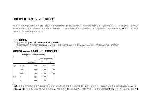
SPSS作业8:二项Logistic回归分析为研究和预测某商品消费特点和趋势,收集到以往胡消费数据.数据项包括是否购买,性别,年龄和收入水平。
这里采用Logistic回归的方法,是否购买作为被解释变量(0/1二值变量),其余各变量为解释变量,且其中性别和收入水平为品质变量,年龄为定距变量。
变量选择采用Enter方法,性别以男为参照类,收入以低收入为参照类。
(一)基本操作:(1)选择菜单Analyz e-Regression-Binary Logistic;(2)选择是否购买作为被解释变量到Dependent框中,选其余各变量为解释变量到Covariates框中,采用Enter方法,结果如下:消费的二项Logistic分析结果(一)(强制进入策略)Categorical Variables CodingsFrequency Parameter coding (1) (2)收入低收入132 .000 .000中收入144 1.000 。
000高收入155 。
000 1。
000性别男191 。
000女240 1.000分析:上表显示了对品质变量产生虚拟变量的情况,产生的虚拟变量命名为原变量名(编码)。
可以看到,对收入生成了两个虚拟变量名为Income(1)和Income(2),分别表示是否中收入和是否高收入,两变量均为0时表示低收入;对性别生成了一个虚拟变量名为Gedder(1),表示是否女,取值为0时表示为男。
消费的二项Logistic 分析结果(二)(强制进入策略)Block 0: Beginning BlockClassification Table a,bObserved Predicted是否购买 Percentage Correct不购买购买Step 0是否购买不购买 269 0 100。
购买162。
0 Overall Percentage62。
4a 。
Constant is included in the model 。
随机过程2016quiz及答案2

Stochastic Processes Name(Print):Fall2016Quizz2:The Laplace Award07/12/16Time Limit:100Minutes Advisor NameThis quiz contains9pages(including this cover page)and8problems.Check to see if any pages are missing.Enter all requested information on the top of this page,and put your initials on the top of every page,in case the pages become separated.Try to answer as many problems as you can.The following rules apply:•Mysterious or unsupported answers will notreceive full credit.A correct answer,unsup-ported by calculations,explanation,or algebraicwork will receive no credit;an incorrect answersupported by substantially correct calculations andexplanations might still receive partial credit.Do not write in the table to the right.Problem PointsScore 110220320420510610710810Total:110随机过程2016quiz及答案1.(10points)When three fair six-sided dice are rolled,what is the probability that the sum ofthe total numbers will be10?2.(20points)Given a random variable X∼P ois(λ)(a)(10points)For any function g,show the Stein-Chen identity for the Poisson:E[Xg(X)]=λE[g(X+1)].(b)(10points)Using the Stein-Chen identity to compute the third moment E(X3).3.(20points)Let a random variable X be Hypergeometric with parameters w,b,n .(a)(10points)Find E X2(b)(10points)Use the result of (a)to find the variance of X .4.(20points)Given a random variable X∼Expo(λ).Find E(X|X<1)in two different ways:(a)(10points)by calculus,working with the conditional PDF of X given X<1.(b)(10points)without calculus,by expanding E(X)using the law of total expectation.5.(10points)A chicken lays N eggs,where N∼P ois(λ).Each egg hatches a chick with proba-bility p,independently.Let X be the number which hatch,so X|N=n∼Bin(n,p).Find the correlation between N(the number of eggs)and X(the number of eggs which hatch).Simplify;yourfinal answer should work out to a simple function of p.6.(10points)The Gumbel distribution is the distribution of−log(X)with X∼Expo(1).(a)(5points)Find the CDF of the Gumbel distribution.(b)(5points)Let X1,X2,...be i.i.d.Expo(1)and let M n=max(X1,...,X n).Show thatM n−log(n)converges in distribution to the Gumbel distribution,i.e.,as n→∞,the CDF of M n−log(n)converges to the Gumbel CDF.7.(10points)Suppose that there are N distinct types of coupons and that,independently of pasttypes collected,each new one obtained is type j with probability p j=1N .Find the expectedvalue and variance of the number of different types of coupons that appear among thefirst n collected.8.(10points)A scientist makes two measurements X,Y,considered to be independent standardNormal r.v.s,i.e.,X∼N(0,1).Find the correlation between the larger and smaller of the values,i.e.,Corr(max(X,Y),min(X,Y)).Probability&Stochastic Processes:Solution of Quizz2December7,20151.Solution:We use three methods to solve the problem.Method1:Just as one die has six outcomes and two dice have62=36outcomes,the experiment of rolling three dice has63=216outcomes.Rolling each die we can get1,2,3,4,5,or6.Thus there are six ways to obtain a sum of10:10=6+3+1=6+2+2=5+3+2=4+4+2=4+3+3=1+4+5.When three different numbers form the partition,such as10=6+3+1,there are3!=6different ways of permuting these numbers.When two different numbers form the partition,such as10=4+4+2,there are 3!/2=3different ways of permuting these numbers.Thus the event that the sum of the total numbers will be10count toward6×3+3×3=27outcomes in the sample space.Thus the probability isPr(the sum of the total numbers will be10)=27216=18.Method2:Let X i be the number of dice i.Then our problem is equal tofind the number of all available solutions of the following problem:X1+X2+X3=10,1≤X1,X2,X3≤6,X1,X2,X3∈Z.First,we do not consider the constraints that X1,X2,X3≤6,then the problem have92=36solutions.Now we consider X1,X2,X3≤6,then7+1+2and8+1+1should be eliminated,so the number of available solutions is36−3!−3=27.Method3:Use the definitions in method2,1≤X1≤6⇒4≤X2+X3≤9.The outcomes satisfy{X2+X3≤3}∪{X2+X3≥10}are1+1,1+2,4+6,5+5,5+6,6+6,thus the probability isPr({X2+X3≤3}∪{X2+X3≥10})=1+2+2+1+2+162=14.⇒Pr(4≤X2+X3≤9)=1−14=34.Given X2,X3,X3can only chosen to be10−X2−X3,the conditional probability is16,thus we get theanswer14×16=124.2.Solution:1(a)The PMF of X is P X (X =k )=e −λλkk !,k =0,1,2,....By LOTUS,E [Xg (X )]=∞k =0kg (k )P X (X =k )=∞k =0kg (k )e −λλkk !=∞ k =1kg (k )e −λλk k !=λ∞k =1g (k )e −λλk −1(k −1)!=λ∞ k =0g (k +1)e −λλkk !=λ∞k =0g (k +1)P X (X =k )=λE [g (X +1)](b)Using the Stein-Chen identity,E X 3 =E X ·X 2=λE (X +1)2 =λE X 2+2X +1=λ E X 2 +2E (X )+1 =λE X 2+2λ2+λwhereE X 2=E (X ·X )=λE (X +1)=λ(E (X )+1)=λ(λ+1)thus we haveE X 3=λ2(λ+1)+2λ2+λ=λ3+3λ2+λ3.Solution:(a)Consider an urn with w white balls and b black balls.We draw n balls out of the urn at random withoutreplacement.Let X be the number of white balls in the sample.Then X ∼HGeom(w,b,n ).Let A i be the event that the i th chosen ball is white,i =1,2,...,n .Let I i be the indicator of A i ,i =1,2,...,n .Since X2= i<j I i I j ,we have EX 2=i<jP (A i A j )By symmetric,P (A i A j )=P (A 1A 2)=P (A 2|A 1)P (A 1)=w −1w +b −1w w +bIt follows thatEX 2=n 2·w −1w +b −1w w +b (b)We haveEX 2=EX (X −1)2=12E X 2 −12E (X ),andE (X )=E (I 1+···+I n )=n i =1E [I i ]=n ·ww +bsince I i ∼Bernww +b,i =1,2,...,n .Combine the above two equations we getE X 2 =n (n −1)w (w −1)(w +b −1)(w +b )+nww +bThen we haveVar (X )=EX2−[E (X )]2=n (n −1)w (w −1)(w +b −1)(w +b )+nww +b−nw w +b24.Solution:(a)By the definition of conditional expectation,E (X |X <1)= ∞0xf (x |X <1)dx =∞xP (X <1|X =x )f (x )P (X <1)dx= 1x f (x )P (X <1)dx = 10x λe −λx 1−e dx =11−e 10λxe −λx dx =11−e −λ 10e −λx dx −xe −λx |10 =1λ−e −λ1−e −λ.(b)By LOTE,E (X )=E (X |X <1)P (X <1)+E (X |X >1)P (X >1)=1/λ.By the memoryless property of Exponential distribution,E (X |X >1)=E (X )+1=1/λ+1.What’s more,P (X <1)=1−e −λ,P (X >1)=e −λ.Thus we getE (X |X <1)=1λ−e −λ1−e −λ.5.Solution:Let Y be the number that do not hatch.Then X |N =n ∼Bin(n,p )and Y |N =n ∼Bin(n,q ).The joint PMF of X and Y isP (X =i,Y =j )=P (X −i |N =i +j )P (N =i +j )= i +j i p i(1−p )j ·e −λλi +j(i +j )!=e −λp (λp )ii !·e −λ(1−p )(λ(1−p ))jj !.Thus X and Y are independent,their marginal PMFs are X ∼Pois(λp )and Y ∼Pois(λ(1−p )).Therefore,Cov (N,X )=Cov (X +Y,X )=Cov (X,X )+Cov (Y,X )=Var (X )+0=λpSince Var(N )=λ,Var(X )=λp ,we getCorr (N,X )=Cov (N,X )Var (N )Var (X )=√p.6.Solution:(a)Let Y =−log (X ),then the CDF of Y isP (Y ≤y )=P (−log (X )≤y )=P X ≥e −y =e −e−y(b)Let Z =M n −log (n ),then the CDF of Z isP (Z ≤z )=P (M n −log (n )≤z )=P (M n ≤log (n )+z )=P (max (X 1,...,X n )≤log (n )+z )=P (X 1≤log (n )+z,...,X n ≤log (n )+z )=P (X 1≤log (n )+z )···P (X n ≤log (n )+z )= 1−e −(log(n )+z )n = 1+−e −z nnSincelimn→∞1+−e−znn=e−e−zwe conclude that the CDF of Z converges to the Gumbel PDF.7.Solution:Let A i be the event that type i coupon appear among thefirst n collected,i=1,2,...,N. Let I i be the indicator of A i,i=1,2,...,N.Let X be the number of different types of coupons that appear among thefirst n collected. Then we have X=I1+I2+···+I N,it follows thatE(X)=E(I1+I2+···+I N)=Ni=1E(I i)=Ni=1P(A i).Since P(A i)=1−P(A c i)=1−(1−p i)n=1−1−1Nn,we getE(X)=N1−1−1Nn.BecauseEX2=i<jP(A i A j),in whichP(A i A j)=P(A i)+P(A j)−P(A i∪A j)=P(A i)+P(A j)−1−PA c i A c j=21−1−1Nn−(1−(1−p i−p j)n)=1−21−1n+1−2n,we haveEX2=N21−21−1Nn+1−2Nn.Using EX2=EX(X−1)2,we getEX2=N2−N(2N−1)1−1Nn+N(N−1)1−2Nn,it follows thatVar(X)=N1−1n−N21−12n+N(N−1)1−2n.8.Solution:Let M=max(X,Y),L=min(X,Y).First,we compute Cov(M,L)usingCov(M,L)=E(ML)−E(M)E(L).We haveE(ML)=E(XY)=E(X)E(Y)=0.By X−Y∼N(0,2),we can get E(|X−Y|)=2√π.CombineE(M)+E(L)=E(M+L)=E(X+Y)=E(X)+E(Y)=0andE(M)−E(L)=E(M−L)=E(|X−Y|)=2√π,we getE(M)=1√π,E(L)=−1√πThus we haveCov(M,L)=1π.Now we compute Var(M)and Var(L).By symmetry of the Normal,(X,Y)has the same distribution as (X,Y),so Var(M)=Var(L).SinceE(X−Y)2=Var(X−Y)=2andE(X−Y)2=E(M−L)2=EM2+EL2−2E(ML)=EM2+EL2,we get EM2+EL2.Then we haveVar(M)=Var(L)=1−−1√π2=1−1π.Finally,we can getCorr(M,L)=Cov(M,L)Var(M)Var(L)=1π−1.。
Aigner-Lovell-Schmidt-JE1977-ALS
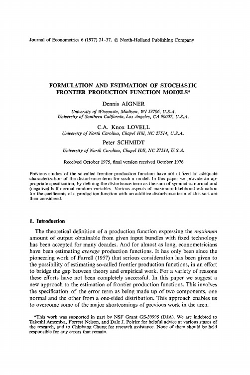
Peter SCHMIDT
University of North Carolina, Chapel Hill, NC 27514, U.S.A. Received October 1975, final version received October 1976 Previous studies of the so-called frontier production function have not utilized an adequate characterization of the disturbance term for such a model. In this paper we provide an appropriate specification, by defining the disturbance term as the sum of symmetric normal and (negative) half-normal random variables. Various aspects of maximum-likelihood estimation for the coefficients of a production function with an additive disturbance term of this sort are then considered.
subject to yi 6 f(xi; p), which is a linear programming problem if f(xi; p) is linear in 1. Alternatively, they suggest minimization of
subject to the same constraint, which is a quadratic programming problem if f(Xi; fl) is linear. Obviously, something magical has happened in moving from (1) to either of these ‘estimation’ methods: In order to characterize differences in output among firms with identical input vectors or to explain how a given firm’s output lies below the ‘frontier’, f(ni, fi), a disturbance term has been implicitly assumed. One problem with these approaches is extreme sensitivity to outliers. This has led to the development of so-called ‘probabilistic’ frontiers [Timmer (1971), Dugger (1974)] which are estimated by the same types of mathematical programming techniques discussed above, except that some specified proportion of the observations is allowed to lie above the frontier. The selection of this proportion is essentially arbitrary, lacking explicit economic or statistical justifi-
决策理论与方法试卷答案4套
咨询后的期望值为:
∑3
E = EiP(Hi ) = 20.6 > 5
i =1
所以应该咨询后生产。
(3)完全情报价值: EVPI = 0.5 × 0 + 0.3×10 + 0.2 × 40 = 11
解:
(1)如果不进行咨询,有期望值准则: E(a1) = 20 , E(a2 ) = 20 , E(a3) = 10
应采取大批量生产方案 a1 或中批量生产 a2 。 (2)进行咨询,根据全概率公式,分别求出咨询后销售状态结果值:
由全概公式:
∑3
P(H1) = P(θi )P(H1 θi ) = 0.5 × 0.4 + 0.3 × 0.3 + 0.2 × 0.3 = 0.35
试卷代码:03A13 课程名称:决策理论与方法
授课对象:042 管理类 适用对象:042 管理类
一、简答题. (要求简要叙述,本题 10 分)
答: 决策的一般过程:发现与分析问题;确定决策目标;拟定各种可行的备择方案; 分析、比较各种备择方案;从中选择最优方案;决策的执行、反馈与调整。
二、计算题. (要求写出详细计算过程,本题 20 分)
五、仿真计算题. (要求写出详细计算过程,本题 10 分)
解:
随机数的产生:
Zi
=
(25Zi −1
+
5) mod(64) ,其中
Z10
=
3,
Z 20
=1,
Ri
=
Zi 64
随机变量序列:
凸优化一阶和二阶条件的证明
2
First and second order characterizations of convex functions
Theorem 2. Suppose f : Rn → R is twice differentiable over an open domain. Then, the following are equivalent: (i) f is convex. (ii) f (y ) ≥ f (x) + ∇f (x)T (y − x), for all x, y ∈ dom(f ). (iii) ∇2 f (x) 0, for all x ∈ dom(f ).
• The theorem simplifies many basic proofs in convex analysis but it does not usually make verification of convexity that much easier as the condition needs to hold for all lines (and we have infinitely many). • Many algorithms for convex optimization iteratively minimize the function over lines. The statement above ensures that each subproblem is also a convex optimization problem. 4
1.4
Examples of multivariate convex functions
• Affine functions: f (x) = aT x + b (for any a ∈ Rn , b ∈ R). They are convex, but not strictly convex; they are also concave: ∀λ ∈ [0, 1], f (λx + (1 − λ)y ) = aT (λx + (1 − λ)y ) + b = λaT x + (1 − λ)aT y + λb + (1 − λ)b = λf (x) + (1 − λ)f (y ). In fact, affine functions are the only functions that are both convex and concave. • Some quadratic functions: f (x) = xT Qx + cT x + d. – Convex if and only if Q 0. 0.
事件研究法详解(event_study)
• Technique mainly used in corporate. • Simple on the surface, but there are a lot of issues. • Long history in finance:
– First paper that applies event-studies, as we know them today: Fama, Fisher, Jensen, and Roll (1969) for stock splits. – Today, we find thousands of papers using event-study methods.
Short and long horizon studies have different goals: – Short horizon studies: how fast information gets into prices. – Long horizon studies: Argument for inefficiency or for different expected returns (or a confusing combination of both)
Classic References
• Brown and Warner (1980, 1985): Short-term performance studies • Loughran and Ritter (1995): Long-term performance study. • Barber and Lyon (1997) and Lyon, Barber and Tsai (1999): Longterm performance studies. • Eckbo, Masulis and Norli (2000) and Mitchell and Stafford (2000): Potential problems with the existing long-term performance studies. • Ahern (2008), WP: Sample selection and event study estimation. • Updated Reviews: M.J. Seiler (2004), Performing Financial Studies: A Methodological Cookbook. Chapter 13. Kothari and Warner (2006), Econometrics of event studies, Chapter 1 in Handbook of Corporate Finance: Empirical Corporate Finance.
2023年计量经济学英文重点知识点考试必备
第一章1.Econometrics(计量经济学):the social science in which the tools of economic theory, mathematics, and statistical inference are applied to the analysis of economic phenomena.the result of a certain outlook on the role of economics, consists of the application of mathematical statistics to economic data to lend empirical support to the models constructed by mathematical economics and to obtain numerical results.2.Econometric analysis proceeds along the following lines计量经济学分析环节1)Creating a statement of theory or hypothesis.建立一种理论假说2)Collecting data.搜集数据3)Specifying the mathematical model of theory.设定数学模型4)Specifying the statistical, or econometric, model of theory.设置记录或经济计量模型5)Estimating the parameters of the chosen econometric model.估计经济计量模型参数6)Checking for model adequacy : Model specification testing.核查模型旳合用性:模型设定检查7)Testing the hypothesis derived from the model.检查自模型旳假设8)Using the model for prediction or forecasting.运用模型进行预测●Step2:搜集数据➢Three types of data三类可用于分析旳数据1)Time series(时间序列数据):Collected over a period of time, are collected at regular intervals.准时间跨度搜集得到2)Cross-sectional截面数据:Collected over a period of time, are collected at regular intervals.准时间跨度搜集得到3)Pooled data合并数据(上两种旳结合)●Step3:设定数学模型1.plot scatter diagram or scattergram2.write the mathematical model●Step4:设置记录或经济计量模型➢C LFPR is dependent variable应变量➢C UNR is independent or explanatory variable独立或解释变量(自变量)➢W e give a catchall variable U to stand for all these neglected factors➢In linear regression analysis our primary objective is to explain the behavior of the dependent variable in relation to the behavior of one or more other variables, allowing for the data that the relationship between them is inexact.线性回归分析旳重要目旳就是解释一种变量(应变量)与其他一种或多种变量(自变量)只见旳行为关系,当然这种关系并非完全对旳●Step5:估计经济计量模型参数➢In short, the estimated regression line gives the relationship between average CLFPR and CUNR 简言之,估计旳回归直线给出了平均应变量和自变量之间旳关系➢That is, on average, how the dependent variable responds to a unit change in the independent variable.单位因变量旳变化引起旳自变量平均变化量旳多少。
- 1、下载文档前请自行甄别文档内容的完整性,平台不提供额外的编辑、内容补充、找答案等附加服务。
- 2、"仅部分预览"的文档,不可在线预览部分如存在完整性等问题,可反馈申请退款(可完整预览的文档不适用该条件!)。
- 3、如文档侵犯您的权益,请联系客服反馈,我们会尽快为您处理(人工客服工作时间:9:00-18:30)。
Journal of Communication and Computer 8(20 1 1)7 l 6—7 1 9 First 0rder Stochastic Dominance in Truncated Log—Normal Distributions
Almaraz Luengo Elena - ,.Department ofStatistic and Operational Research,Fac Sciences Mathematics,University Complutense ofMadrid,Madrid 28040 Spain 2.SantaAnaYSan RafaelFEMDL,Madrid28028,Spain
Received:May 1 3,20 1 1/Accepted:May 1 8,20 1 1/Published:September 30,20 1 1 Abstract:We analyze first order stochastic dominance between log—Normal truncated distributions,studying the relations between the original log—Normal distributions and verifying if these relations survive with the truncation.We derive sufficient and necessary conditions about stochastic dominance between truncated log-Normal distributions knowing some properties that verify the parameters of the original non・-truncated distributions even in cases in which there is no relationship between the original non--truncated distributions.
Key words:Log-Normal distribution,stochastic dominance,truncated distribution 1.1ntroduction Suppose that is the return of an investment.we define Y such that Y=Ln If Y is normally distributed. N( f,o-),where E(LnX)= andcr(LnX)= , then X itself wil1 be lognormal distributed.Log.Normal distribution is a positive distribution skewed to the right. In this paper we analyze the first order dominance criterion applied to log-Normal distributions.There exists first order stochastic dominance(FSD1 between two log—Normal distilbutions only when they have the same standard deviation.We will show that if we build the truncated distributiOns we can obtain FSD between them even in cases in which the original log—Normal distilbutions do not have relation in FSD sense.For the purpose of this work we need to define the first order stochastic dominance(FSD)concept:Let F and G be the cumulative distributions function of two random variables X and Y X dominates Y by FSD and we denote X Fs if and only if F《x)<G(x) for all x∈R
C0rresponding author:Almaraz Luengo Elena,Ph.D., professor,research fields:stochastic processes,portfolio selection.E—mail:ealmarazluengo@mat.ucm.es.
and with at least one point in which the inequality is strict(more about FSD see Refs_[1]and[2]). In section 2 we study the main concepts of truncated distributions.In section 3 we study log-Norma1 and truncated log—Norlnal distributions.In section 4 we derive the principal results and in section 5 the conclusions are explained.
2.Truncated Distributions Definition 1 Given an one—dimensionaf random variable Xdefined in a probability space fQ.A P)with P【X E I1 E(o.1).being T an element of the Borel ̄ a-algebra over .we define de truncated distribution of X as the conditional distribution P}X xf xE T1 E fo 11 definedover Definition 2 IfF is the distribution ofX,we define the truncatedfunction FofF inpoints A andB口 if x<A
, A <B (1) 1, if x≥B with A and B the truncation points verifying F and F 一 2.The truncation can be symmetric First Order Stochastic Dominance in Truncated Log-Normal Distributions 《Ocl=of2).or asymmetric:《oc ≠of2). Definition 3 If the random variable X is continuous, with density./ ̄*
,we define the truncated density as:
:』 ,… 厂( ):{』/ (x) ’ ~… (2)
l l 0, in—other—case
3.Lognormal Distributions:Basic Concepts Normal distribution is most often assumed to describe the random variation that Occurs in the data from many scientific areas and in some occasions can be easier to handle than the log.Normal distribution in mathematics context,however,many measurements show a more or less skewed distribution.Skewed distributions are particularly common when mean values are low,variances large,and values cannot be negative,for example in economic context,because the price of the assets cannot be negative and in many distributions of ratio of returns it exists a positive asymmetry that appears in the log—Normal distribution and not in the Normal distribution,(more about log—Normal distributions in Refs.[4]and[5]). When we compare two log.Normal distributions
F-LN( 1, l and G~LN(At2, 2),we can get the following conclusion:F dominates G by FSD if and only if Atl>At2 and l= 2(see Refi[63). Definition 4 A random variable X is log-Normal with parameters At and o-(X-LN(/ ̄.o)).if the random variable Y=Ln x is Normal with parameters with parameters and o(Y-N(p o-)).For f>o: P t]=P[LnX<_Lnt] I , Lnt一 being the
distribution function of the Narmal Standard distribution,and so the density is: