hurst 程序
自相似流量模拟的Hurst参数实时计算

0引言在网络信息及通信技术发展的过程中,网络流量模型一直是研究的重点,二十世纪七八十年代,人们主要采用PSTN 模型对网络流量的到达过程进行研究,由泊松模型的基本假定条件可知,伴随时间的延续和数据的累积,累计流量应该趋近平均值,然而取得的结果却与此有很大差异。
Leland 和Willinger 等人收集了Bellcore 实验室在1989到1992年之间的各种Ethernet LAN 的数据,证明了传统用泊松到达传输来分析流量的假定是不充分的,需要新的信源模型。
Berkeley 实验室的Vern 等,在长期的研究中发现绝大部分的TCP 过程,具有时间尺度上的非常明显的自相似性特点,这并不同于泊松过程,主要表现为流量的突发性。
因此,对网络流量数据包的到达过程来建立模型时,应当结合自相似的过程进行建立。
基于各种测试的统计,他们得到Ethernet 的信源是自相似的,并测得自相似的重要参数Hurst 的值是0.9。
1自相似的数学定义对于自相似过程的研究始于本世纪中叶,对于一个系统来说,其自相似性主要是从不同的时空尺度上来看某种过程或结构的特征都具有相似性。
此外,各整体之间,或者是部分与部分之间,也会存在相似性。
一般情况下自相似性有比较复杂的表现形式而不是局域放大倍数以后简单地和整体完全重合。
自相似性应用领域非常广泛,包括天文学、地理学、电子学、化学以及环境科学等众多领域。
自相似性是跨尺度重复性,它可以产生出具有结构和规则的统计热性,这是对自相似性现象的直观描述。
在统计意义上,自相似过程主要表现为尺度不变性的随机过程。
基于此,这种过程实际上可以认为是在随机过程的基础上引入了分形。
对于随机过程X (t ),(-∞<t+∞)假设在时间方面对X (t )进行扩展与压缩时,其统计特性并不发生变化,也就是说X (t )满足X (t )D =a -HX (at ),则这一过程也就是统计自相似的,其中“=”主要体现在统计意义上。
Huffman编码完整程序

本文档包含huffman编码,解码,译码,生成huffman树的所有程序。
实验代码为://..................huffmantree..............................//typedef struct{int weight;int parent;int left;int right;}HuffmanTree;typedef char *HuffmanCode;void SelectNode(HuffmanTree *ht,int n,int *bt1,int *bt2){HuffmanTree *ht1,*ht2,*t;ht1=ht2=NULL;for(int i=1;i<=n;i++){if(! ht[i].parent){if(ht1==NULL){ht1=ht+i;continue;}if(ht2==NULL){ht2=ht+i;if(ht1->weight > ht2->weight){t=ht2;ht2=ht1;ht1=t;}continue;}if(ht1 && ht2){if(ht[i].weight <= ht1->weight){ht2=ht1;ht1=ht+1;}else if(ht[i].weight < ht2->weight){ht2=ht+i;}}}}if(ht1 > ht2){*bt2=ht1-ht;*bt1=ht2-ht;}else{*bt1=ht1-ht;*bt2=ht2-ht;}}void CreatTree(HuffmanTree *ht,int n,int *w) {int i,m=2*n-1;int bt1,bt2;if(n<=1) return;for(i=1;i<=n;i++){ht[i].weight=w[i-1];ht[i].parent=0;ht[i].left=0;ht[i].right=0;}for(;i<=m;++i){ht[i].weight=0;ht[i].parent=0;ht[i].left=0;ht[i].right=0;}for(i=n+1;i<=m;++i){SelectNode(ht,i-1,&bt1,&bt2);ht[bt1].parent=i;ht[bt2].parent=i;ht[i].left=bt1;ht[i].right=bt2;ht[i].weight=ht[bt1].weight+ht[bt2].weight;}}void HuffmanCoding(HuffmanTree *ht,int n,HuffmanCode *hc) {char *cd;int start,i,current,parent;cd=(char *)malloc(sizeof(char)*n);cd[n-1]='\0';for(i=1;i<=n;i++){start=n-1;current=i;parent=ht[current].parent;while(parent){if(current==ht[parent].left)cd[--start]='0';elsecd[--start]='1';current=parent;parent=ht[parent].parent;}hc[i-1]=(char *)malloc(sizeof(char)*(n-start));strcpy(hc[i-1],&cd[start]);}free(cd);}void Encode(HuffmanCode *hc,char *alphabet,char *str,char *code) {int len=0,i=0,j;code[0]='\0';while(str[i]){j=0;while(alphabet[j] != str[i])j++;strcpy(code+len,hc[j]);len=len+strlen(hc[j]);i++;}code[len]='\0';}void Decode(HuffmanTree *ht,int m,char *code,char *alphbet,char *decode) {int position=0,i,j=0;m=2*m-1;while(code[position]){for(i=m;ht[i].left && ht[i].right;position++){if(code[position]=='0')i=ht[i].left;elsei=ht[i].right;}decode[j]=alphbet[i-1];j++;}decode[j]='\0';}主函数为:int main(){int i,n=4,m;char test[]="DBDBDABDCDADBDADBDADACDBDBD";char code[100],code1[100];char alphabet[]={'A','B','C','D'};int w[]={5,7,2,13};HuffmanTree *ht;HuffmanCode *hc;m=2*n-1;ht=(HuffmanTree *)malloc((m+1)*sizeof(HuffmanTree));if(! ht){cout<<"failed !"<<endl;exit(0);}hc=(HuffmanCode *)malloc(n*sizeof(char *));if(! hc){cout<<"failed !"<<endl;exit(0);}CreatTree(ht,n,w);HuffmanCoding(ht,n,hc);for(i=1;i<=n;i++)cout<<"alpabet:"<<alphabet[i-1]<<" weight:"<<ht[i].weight<<" code:"<<hc[i-1]<<endl;Encode(hc,alphabet,test,code);cout<<"the string is:"<<alphabet<<endl;cout<<"now encode is:"<<code<<endl;Decode(ht,n,code,alphabet,code1);cout<<endl<<code<<endl;cout<<code1<<endl;return 0;}。
分形布朗运动和hurst指数

分形布朗运动和hurst指数
分形布朗运动是一种随机过程,其特性与布朗运动相似,但具有更复杂的分形结构。
布朗运动是指微观粒子在液体或气体中由于受到分子的不断碰撞而进行的无规则、连续且随机的运动。
而分形布朗运动则是在这种运动过程中引入了分形结构,使得其具有更为复杂的运动模式。
Hurst指数是用来描述分形布朗运动的一个重要参数。
它表示分形布朗运动在时间序列上的长期依赖性或持久性。
Hurst指数的值介于0和1之间,其中0.5表示随机游走,小于0.5表示负持久性,即过去的变化趋势对未来的影响逐渐减弱,而大于0.5则表示正持久性,即过去的变化趋势对未来的影响逐渐增强。
在金融领域中,分形布朗运动和Hurst指数被广泛应用于模拟股票价格等金融时间序列。
由于股票价格具有分形结构和持久性,因此分形布朗运动可以很好地描述股票价格的波动特征。
通过估计Hurst指数,我们可以了解股票价格的波动趋势和未来价格的变化情况。
除了金融领域,分形布朗运动和Hurst指数还在其他领域得到广泛应用。
例如,在地球物理学中,它们被用于模拟地震和海浪等自然现象;在生物学中,它们被用于描述生物种群的增长和变化趋势等。
此外,分形布朗运动和Hurst 指数还被应用于图像处理、信号处理等领域。
总之,分形布朗运动是一种具有复杂分形结构的随机过程,其特性与布朗运动相似但更为复杂。
Hurst指数是描述分形布朗运动的一个重要参数,可以用来估计时间序列的持久性和变化趋势。
在金融、地球物理学、生物学等领域中,分形布朗运动和Hurst指数得到了广泛应用,为我们提供了更准确、更有效的分析方法和工具。
希尔伯特-黄变换说明及程序(标准程序)

目录∙ 1 本质模态函数(IMF)∙ 2 经验模态分解(EMD)∙ 3 结论∙ 4 相关条目∙ 5 参考文献∙ 6 外部链接[编辑]本质模态函数(IMF)任何一个资料,满足下列两个条件即可称作本质模态函数。
⒈局部极大值(local maxima)以及局部极小值(local minima)的数目之和必须与零交越点(zero crossing)的数目相等或是最多只能差1,也就是说一个极值后面必需马上接一个零交越点。
⒉在任何时间点,局部最大值所定义的上包络线(upper envelope)与局部极小值所定义的下包络线,取平均要接近为零。
因此,一个函数若属于IMF,代表其波形局部对称于零平均值。
此类函数类似于弦波(sinusoid-like),但是这些类似于弦波的部分其周期与振幅可以不是固定。
因为,可以直接使用希尔伯特转换,求得有意义的瞬时频率。
[编辑]经验模态分解(EMD)EMD算法流程图建立IMF是为了满足希尔伯特转换对于瞬时频率的限制条件之前置处理,也是一种转换的过程。
我们将IMF来做希尔伯特转换可以得到较良好的特性,不幸的是大部分的资料并不是IMF,而是由许多弦波所合成的一个组合。
如此一来,希尔伯特转换并不能得到正确的瞬时频率,我们便无法准确的分析资料。
为了解决非线性(non-linear)与非稳态(non-stationary)资料在分解成IMF时所遇到的困难,便发展出EMD。
经验模态分解是将讯号分解成IMF的组合。
经验模态分解是借着不断重复的筛选程序来逐步找出IMF。
以讯号为例,筛选程序的流程概述如下:步骤 1 : 找出中的所有局部极大值以及局部极小值,接着利用三次样条(cubic spline),分别将局部极大值串连成上包络线与局部极小值串连成下包络线。
步骤 2 : 求出上下包络线之平均,得到均值包络线。
步骤 3 : 原始信号与均值包络线相减,得到第一个分量。
步骤 4 : 检查是否符合IMF的条件。
hurst_exponent_and_financial_market_predictability
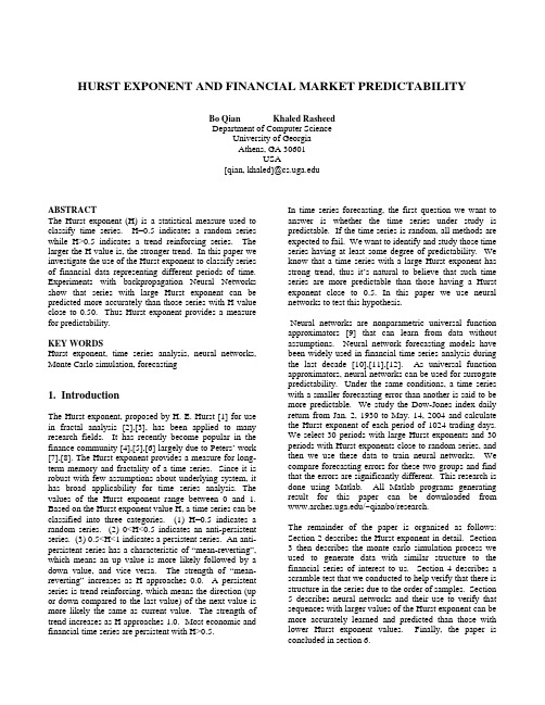
HURST EXPONENT AND FINANCIAL MARKET PREDICTABILITYBo Qian Khaled RasheedDepartment of Computer ScienceUniversity of GeorgiaAthens, GA 30601USA[qian, khaled]@ABSTRACTThe Hurst exponent (H) is a statistical measure used to classify time series. H=0.5 indicates a random series while H>0.5 indicates a trend reinforcing series. The larger the H value is, the stronger trend. In this paper we investigate the use of the Hurst exponent to classify series of financial data representing different periods of time. Experiments with backpropagation Neural Networks show that series with large Hurst exponent can be predicted more accurately than those series with H value close to 0.50. Thus Hurst exponent provides a measure for predictability.KEY WORDSHurst exponent, time series analysis, neural networks, Monte Carlo simulation, forecasting1. IntroductionThe Hurst exponent, proposed by H. E. Hurst [1] for use in fractal analysis [2],[3], has been applied to many research fields. It has recently become popular in the finance community [4],[5],[6] largely due to Peters’ work [7],[8]. The Hurst exponent provides a measure for long-term memory and fractality of a time series. Since it is robust with few assumptions about underlying system, it has broad applicability for time series analysis. The values of the Hurst exponent range between 0 and 1. Based on the Hurst exponent value H, a time series can be classified into three categories. (1) H=0.5 indicates a random series. (2) 0<H<0.5 indicates an anti-persistent series. (3) 0.5<H<1 indicates a persistent series. An anti-persistent series has a characteristic of “mean-reverting”, which means an up value is more likely followed by a down value, and vice versa. The strength of “mean-reverting” increases as H approaches 0.0. A persistent series is trend reinforcing, which means the direction (up or down compared to the last value) of the next value is more likely the same as current value. The strength of trend increases as H approaches 1.0. Most economic and financial time series are persistent with H>0.5. In time series forecasting, the first question we want to answer is whether the time series under study is predictable. If the time series is random, all methods are expected to fail. We want to identify and study those time series having at least some degree of predictability. We know that a time series with a large Hurst exponent has strong trend, thus it’s natural to believe that such time series are more predictable than those having a Hurst exponent close to 0.5. In this paper we use neural networks to test this hypothesis.Neural networks are nonparametric universal function approximators [9] that can learn from data without assumptions. Neural network forecasting models have been widely used in financial time series analysis during the last decade [10],[11],[12]. As universal function approximators, neural networks can be used for surrogate predictability. Under the same conditions, a time series with a smaller forecasting error than another is said to be more predictable. We study the Dow-Jones index daily return from Jan. 2, 1930 to May. 14, 2004 and calculate the Hurst exponent of each period of 1024 trading days. We select 30 periods with large Hurst exponents and 30 periods with Hurst exponents close to random series, and then we use these data to train neural networks. We compare forecasting errors for these two groups and find that the errors are significantly different. This research is done using Matlab. All Matlab programs generating result for this paper can be downloaded from /~qianbo/research.The remainder of the paper is organised as follows: Section 2 describes the Hurst exponent in detail. Section 3 then describes the monte carlo simulation process we used to generate data with similar structure to the financial series of interest to us. Section 4 describes a scramble test that we conducted to help verify that there is structure in the series due to the order of samples. Section 5 describes neural networks and their use to verify that sequences with larger values of the Hurst exponent can be more accurately learned and predicted than those with lower Hurst exponent values. Finally, the paper is concluded in section 6.2. Hurst exponent and R/S analysisThe Hurst exponent can be calculated by rescaled range analysis (R/S analysis). For a time series, X = X 1, X 2, … Xn, R/S analysis method is as follows:(1) Calculate mean value m.∑==ni inXm 11(2) Calculate mean adjusted series YY t = X t – m, t = 1, 2, …, n(3) Calculate cumulative deviate series Z∑==ti i t Y Z 1, t = 1, 2, …, n(4) Calculate range series RR t = max(Z 1, Z 2, …, Z t ) – min(Z 1, Z 2, …, Z t ) t = 1, 2, …, n(5) Calculate standard deviation series S∑=−=ti i t u X t S 12)(1 t = 1, 2, …, nHere u is the mean value from X 1 to X t .(6) Calculate rescaled range series (R/S)(R/S)t = R t /S t t = 1, 2, …, nNote (R/S)t is averaged over the regions [X 1, X t ], [X t+1, X 2t ] until [X (m-1)t+1, X mt ] where m=floor(n/t). In practice, to use all data for calculation, a value of t is chosen that is divisible by n.Hurst found that (R/S) scales by power-law as time increases, which indicates(R/S)t = c*t HHere c is a constant and H is called the Hurst exponent. To estimate the Hurst exponent, we plot (R/S) versus t in log-log axes. The slope of the regression line approximates the Hurst exponent. For t<10, (R/S)t is not accurate, thus we shall use a region of at least 10 values to calculate rescaled range. Figure 2.1 shows an exampleof R/S analysis.Figure 2.1. R/S analysis for Dow-Jones daily returnfrom 11/18/1969 to 12/6/1973In our experiments, we calculated the Hurst exponent for each period of 1024 trading days (about 4 years). We use t = 24, 25, …, 210 to do regression. In the financial domain, it is common to use log difference as daily return. This is especially meaningful in R/S analysis since cumulative deviation corresponds to cumulative return. Figure 2.2 shows the Dow-Jones daily return from Jan. 2, 1930 to May 14, 2004. Figure 2.3 shows the corresponding Hurst exponent for this period. In this period, Hurst exponent ranges from 0.4200 to 0.6804. We also want to know what the Hurst exponent would be for a random series inour condition.Figure 2.2. Dow-Jones daily return from 1/2/1930 to 5/14/2004YearHu r s t E x p o n e n tFigure 2.3. Hurst exponent for Dow-Jones daily return from 1/2/1930 to 5/14/20043. Monte Carlo simulationFor a random series, Feller [13] gave expected (R/S)tformula as 3.1.E((R/S)t ) = (n*π/2)0.50(3.1)However, this is an asymptotic relationship and is onlyvalid for large t. Anis and Lloyd [14] provided thefollowing formula to overcome the bias calculated from(3.1) for small t:∑−=−Γ−Γ=11/)(*)))*5.0(*/())1(*5.0(()/((t r r r t t t t S R E π(3.2)For t>300, it is difficult to calculate the gamma functionby most computers. Using Sterling’s function, formula(3.2) can be approximated by:∑−=−−=11/)(*50.0)2/*())/((t r r r t t tS R E π (3.3)Peters [8] gave equation (3.4) as a correction for (3.2).∑−=−−−=11/)(*50.0)2/*(*)/)5.0(())/((t r r r t t t t tS R E π(3.4)We calculate the expected (R/S) values for t=24, 25,…,210and do least squares regression at significance levelα=0.05. Results are shown in table 3.1.log2(E(R/S)) log2(t) Feller Anis Peters4 0.7001 0.6059 0.57095 0.8506 0.7829 0.7656 6 1.0011 0.9526 0.94407 1.1517 1.1170 1.11278 1.3022 1.2775 1.2753 9 1.4527 1.4345 1.4340 10 1.6032 1.5904 1.5902 Regression Slope (H) 0.5000 ±5.5511e-016 0.5436 ± 0.0141 0.5607 ± 0.0246Table 3.1. Hurst exponent calculation from Feller, Anis and Peters formula From table 3.1, we can see that there are some differences between Feller’s, Anis’ and Peters’ formulae. Moreover, their formulae are based on large numbers of data points. In our case, the data is fixed at 1024 points. So what is the Hurst exponent for random series in our case?Fortunately, we can use Monte Carlo simulation to derivethe result. We generate 10,000 Gaussian random series.Each series has 1024 values. We calculate the Hurstexponent for each series and then average them. Weexpect the average number to approximate the true value.We repeated this process 10 times. Table 3.2 below givesthe simulation results. Simulated Hurst Exponent Standard deviation (Std.) 1 0.5456 0.0486 2 0.5452 0.04873 0.5449 0.04884 0.5454 0.04845 0.5456 0.04886 0.5454 0.04817 0.5454 0.04878 0.5457 0.04839 0.5452 0.048410 0.5459 0.0486Mean 0.5454 0.0485Std. 2.8917e-004Table 3.2. Monte Carlo simulations for Hurst exponent of random seriesFrom table 3.2, we can see that in our situation, the Hurst exponent calculated from Monte Carlo simulations is 0.5454 with standard deviation 0.0485. Our result is very close to Anis’ formula. Based on the above simulations, with 95% confidence, the Hurst exponent is in the interval 0.5454 ± 1.96*0.0485, which is between 0.4503 and 0.6405. We choose those periods with Hurst exponent greater than 0.65 and expect those periods to be bearing some structure different from random series. However, since these periods are chosen from a large sample (total 17651 periods), we want to know if there exists true structure in these periods, or just by chance. We run a scramble test for this purpose.4. Scramble testTo test if there exists true structure in the periods withHurst exponent greater than 0.65, we randomly choose 10samples from those periods. For each sample, wescramble the series and then calculate the Hurst exponentfor this scrambled series. The scrambled series has thesame distribution as the original sample except that thesequence is random. If there exists some structure in thesequence, after scrambling the structure will be destroyedand the calculated Hurst exponent should be close to thatof a random series. In our experiment, we scramble eachsample 500 times and then the average Hurst exponent iscalculated. The results are shown in table 4.1 below.Hurst exponent after scrambling Standarddeviation1 0.5492 0.0462 0.5450 0.0473 0.5472 0.0494 0.5454 0.0485 0.5470 0.0486 0.5426 0.0487 0.5442 0.0518 0.5487 0.0489 0.5462 0.04810 0.5465 0.052Mean 0.5462 0.048Table 4.1. The average Hurst exponent on 500scrambling runsFrom table 4.1, we can see that the Hurst exponents afterthe scrambling of samples are all very close to 0.5454which is the number from our simulated random series.Given this result, we can conclude that there must existsome structure in those periods making them differentfrom random series and that scrambling destroys thestructure. We hope this structure can be exploited forprediction. Neural networks, as universal functionapproximators, provide a powerful tool to learn theunderlying structure. They are especially useful when theunderlying rules are unknown. We expect neuralnetworks to discover the structure and thus benefit from it. We use neural network prediction error as a measure of predictability. Below we compare prediction errors of the periods with Hurst exponents greater than 0.65 with those between 0.54 and 0.55.5. Neural networksIn 1943, McClloch and Pitts [15] proposed a computational model simulating neurons. This work is generally thought as the beginning of artificial neural networks research. Rosenblatt [16],[17] popularized the concept of perceptrons and created several perceptron learning rules. However, in 1969, Minsky and Papert [18] pointed that perceptrons cannot solve any non “linearly separable” problems. People knew that multi-layer perceptrons (MLP) can simulate non “linearly separable” functions, but no one knew how to train them. Neural network research was then nearly stopped until 1986. In 1986, Rumelhart [19] used the backpropagation algorithm to train MLP and thus resolved this long obsessed problem among connectionists. Since then neural networks have regained considerable interest from many research fields. Neural networks have become popular in the finance society and the research fund for neural network applications from financial institutions is the second largest [20]. A neural network is an interconnected assembly of simple processing nodes. Each node calculates a summation of weighted inputs and then outputs its transfer function value to other nodes. The Feedforward backpropagation network is the most widely used network paradigm. Using the backpropagation training algorithm, neural network adjusts the weights so that it will minimize the square difference (error) between its observed outputs and their target values. The backpropagation algorithm uses a gradient descent method to find a local minimum on the error surface. It calculates the partial derivative of the square error for each weight. The opposite of these partial derivatives (gradient) gives the direction in which the error decreases most. This direction is called the steepest descent direction. The standard backpropagation algorithm adjusts the weights along the steepest descentdirection. Although the error in the steepest descentdirection is decreased most rapidly, it usually convergesslowly and tends to be stranded due to oscillation. Therefore many backpropagation variants were inventedto improve performance by optimizing direction and step size. To name a few, we have backpropagation withmomentum, conjugate gradient, Quasi-Newton and Levenberg-Marquardt [21]. After training, we can use thenetwork to do prediction given unseen inputs . In neural network forecasting, the first step is data preparation andpre-processing. After training, we can use the network to do prediction given unseen inputs. In neural networkforecasting, the first step is data preparation and pre-processing.5.1. Data preparation and pre-processingFor Dow-Jones daily return data, we calculated the Hurst exponent for each period of 1024 trading days from 1/2/1930 to 5/14/2004. Among the total of 17651 periods, there are 65 periods with Hurst exponents greater than 0.65 and 1152 periods with Hurst exponents between 0.54 and 0.55. Figure 5.3 below shows the histogram of Hurst exponents for all periods.Figure 5.3. Histogram of all calculated HurstexponentsWe randomly chose 30 periods from those with Hurst exponent greater than 0.65 and 30 periods from those with Hurst exponent between 0.54 and 0.55. These two groups of 60 samples constituted our initial data set.Given a time series x1, x2, …, x i, x i+1, how do we construct a vector X i from x1, x2, …, x i to predict x i+1? Taken’s theorem [22] tells us that we can reconstruct the underlying dynamical system by time-delay embedding vectors X i = (x i, x i+τ, x i+2τ,…,x i+(d-1)τ) if we have appropriate d and τ. Here d is called the embedding dimension and τ is called the separation. Using the auto-mutual information and false nearest neighbour methods [23], we can estimate d and τ. We used the TSTOOL [24] package to run the auto-mutual information and false nearest neighbour methods for our 60 data sets. Separations of all data sets are suggested to be 1 by auto-mutual information method. This is consistent with our intuition since we have no reason to use separated values. As for embedding dimension, our data sets are suggested to be from 3 to 5. We shall examine this later.After building the time-delay vector Xi and target value x i+1, we normalized the inputs Xi and output x i+1 to mean 0 and standard deviation 1. We had no need to normalize the output to a limited range, say –0.85 to 0.85, to avoid saturation because we used a linear transfer function in the output layer. We used a commonly used approach to deal with the over-fitting problem in neural networks. We split the data set to three parts for training, validation and testing. The training data are used to adjust the weights through error backpropagation. The validation data are used to stop training when the mean square error in the validation data increases. The network’s prediction performance is judged by the testing data. We used the first 60% of the data for training, the following 20% for validation and the last 20% for testing. In this way, we can have more confidence using the final network model for prediction since the forecasting data follow the testing data directly.5.2 Neural network constructionAlthough neural networks are universal function approximators, we still need to pay much attention to their structure. How many layers should we use? How many nodes should we include in each layer? Which learning algorithm should we choose? In practice, most applications use one hidden layer since there is no apparent advantages for multi-hidden-layer networks over single-hidden-layer networks. Thus we used a single hidden layer network structure in our study. For learning algorithm, we tested the Levenberg-Marquardt, conjugate gradient method, and the backpropagation with momentum algorithms. We find that Levenberg-Marquardt beats the other algorithms consistently in our test samples. We chose the Levenberg-Marquardt learning algorithm with the sigmoid transfer function in the hidden layer and a linear transfer function in the output layer. Now we need to determine the embedding dimension and the number of hidden nodes. A heuristic rule to determine the number of hidden nodes is that the total degrees of freedom of a network should equal one and half of the square root of the total data numbers. Based on this rule, we have the following equation:(#input nodes+1)*(#hidden nodes) + (#hiddennodes+1)*(#output nodes) = 1.5sqrt(#data)(5.2.1) In equation (5.2.1), 1 is for bias node. For dimension 3, we have:(3+1)*(#hidden nodes)+(#hidden nodes+1) = 1.5sqrt(1024)The solution for (#hidden nodes) is 10. Similarly, we find that the number of hidden nodes for dimensions 4 and 5 are 8 and 7 respectively. For each dimension, we examine 5 network structures with the number of hidden nodes adjacent to the number suggested. For example 8, 9, 10, 11, 12 hidden nodes for dimension 3. We randomly choose 5 periods from each group (the group with Hurst exponents greater than 0.65 and the group with Hurst exponents between 0.54 and 0.55) to train each network. Each network is trained 100 times, and then the minimum NRMSE (Normalized Root Mean Square Error) is recorded. NRMSE is defined as:∑∑−−=ii i i i T T T O NRMSE )()(2 (5.2.2)In (5.2.2), O is output value and T is target value.NRMSE gives a performance comparison to the meanprediction method. If we always use the mean value to doprediction, NRMSE will be 1. NRMSE is 0 when allpredictions are correct.Table 5.1-5.3 gives the training results for variousnetwork structures.Dimension 3, Hidden nodes8 9 10 11 12 MIN Std. 1 0.9572 0.9591 0.9632 0.9585 0.9524 0.95240.00392 0.9513 0.9531 0.9560 0.9500 0.9523 0.95000.00233 0.9350 0.9352 0.9332 0.9328 0.9359 0.93280.00134 0.9359 0.9426 0.9383 0.9351 0.9313 0.93130.00425 0.9726 0.9686 0.9652 0.9733 0.9647 0.96470.00406 0.9920 0.9835 0.9892 0.9793 0.9931 0.97930.00597 0.9831 0.9813 0.9725 0.9845 0.9825 0.97250.00488 0.9931 0.9852 0.9832 0.9877 0.9907 0.98320.00409 0.9684 0.9790 0.9773 0.9815 0.9862 0.96840.006610 0.9926 1.0044 1.0047 1.0014 1.0039 0.99260.0051Mean 0.9681 0.9692 0.9683 0.9684 0.9693 0.96270.0042Std. 0.0225 0.0215 0.0221 0.0232 0.0255 0.02070.0015Table 5.1. NRMSE for dimension 3 with hidden nodes8, 9, 10, 11 and 12Dimension 4, Hidden nodes 6 7 8 9 10MIN Std. 1 0.9572 0.9572 0.9557 0.9558 0.9633 0.95570.00312 0.9534 0.9554 0.9523 0.9518 0.9574 0.95180.00233 0.9373 0.9406 0.9414 0.9437 0.9404 0.93730.00234 0.9419 0.9471 0.9392 0.9332 0.9376 0.93320.00525 0.9691 0.9678 0.9597 0.9669 0.9662 0.95970.00376 0.9907 0.9939 0.9836 0.9948 0.9876 0.98360.00467 0.9902 0.9816 0.9872 0.9766 0.9855 0.97660.00538 0.9852 0.9842 0.9802 0.9865 0.9878 0.98020.00299 0.9809 0.9729 0.9722 0.9669 0.9741 0.96690.005010 0.9916 0.9957 0.9991 1.0025 0.9959 0.99160.0041Mean 0.9698 0.9696 0.9671 0.9679 0.9696 0.96370.0038Std. 0.0210 0.0193 0.0204 0.0225 0.0203 0.01960.0012 Table 5.2. NRMSE for dimension 4 with hidden nodes 6, 7, 8, 9 and 10 Dimension 5, Hidden nodes 5 6 7 8 9MIN Std. 1 0.9578 0.9560 0.9617 0.9589 0.9622 0.95600.00262 0.9441 0.9466 0.9456 0.9456 0.9427 0.94270.00153 0.9410 0.9395 0.9449 0.9428 0.9396 0.93950.00234 0.9546 0.9453 0.9414 0.9409 0.9479 0.94090.00565 0.9659 0.9501 0.9671 0.9653 0.9653 0.95010.00716 0.9906 0.9919 0.9898 0.9901 0.9891 0.98910.00107 0.9803 0.9819 0.9805 0.9840 0.9837 0.98030.00178 0.9912 0.9980 1.0009 0.9991 1.0049 0.99120.00509 0.9770 0.9747 0.9742 0.9761 0.9689 0.96890.003210 0.9909 0.9984 0.9975 0.9977 0.9951 0.99090.0031Mean 0.9693 0.9682 0.9704 0.9701 0.9699 0.96500.0033Std. 0.0194 0.0233 0.0220 0.0226 0.0227 0.02170.0020Table 5.3. NRMSE for dimension 5 with hidden nodes5, 6, 7, 8, and 9From table 5.1 to 5.3, we can see that the differences ofNRMSE for nodes within each dimension are very small. The number of hidden nodes with minimum average NRMSE for dimension 3, 4, 5 are 8, 8 and 6 respectively. Thus we use 8, 8, and 6 hidden nodes network for dimension 3, 4, and 5 to do prediction. Each network is trained 100 times and the minimum NRMSE is recorded. Final NRMSE is the minimum of 3 dimensions. Table 5.4 gives NRMSE of our initial 60 samples for two groups.H>0.65 0.55>H>0.54 H>0.650.55>H>0.54 10.9534 0.9863 160.93 0.974720.9729 0.9784 170.9218 0.9738 30.9948 0.9902 180.9256 0.9635 40.9543 0.9754 190.9326 0.957 50.9528 0.9773 200.937 0.9518 60.9518 0.9477 210.9376 0.9542 70.9466 0.9265 220.9402 0.9766 80.9339 0.9598 230.9445 0.9901 90.9299 0.9658 240.9498 0.9777 100.9435 0.9705 250.948 0.9814 110.9372 0.9641 260.9486 0.9778 120.9432 0.9824 270.9451 0.9968 130.9343 0.9557 280.9468 0.9966 140.9338 0.9767 290.9467 0.9977150.9265 0.9793 300.9542 0.9883 Mean 0.9439 0.9731 Std.0.0145 0.0162Table 5.4. NRMSE for two groups We ran the unpaired student’s t test for the null hypothesis that the mean values of the two groups are equal. After calculation, the t statistic is 7.369 and p-value is 7.0290e-010. This indicates the two means are significantly different and the chance of equality is essentially 0. This result confirms that the time series with larger Hurstexponent can be predicted more accurately.6. ConclusionIn this paper, we analyze the Hurst exponent for all 1024-trading-day periods of the Dow-Jones index from Jan.2, 1930 to May 14, 2004. We find that the periods with large Hurst exponents can be predicted more accurately than those with H values close to random series. This suggests that stock markets are not totally random in all periods. Some periods have strong trend structure and this structure can be learnt by neural networks to benefit forecasting.Since the Hurst exponent provides a measure for predictability, we can use this value to guide data selection before forecasting. We can identify time series with large Hurst exponents before we try to build a model for prediction. Furthermore, we can focus on the periods with large Hurst exponents. This can save time and effort and lead to better forecasting.References:[1] H.E. Hurst, Long-term storage of reservoirs: an experimental study, Transactions of the American society of civil engineers, 116, 1951, 770-799.[2] B.B. Mandelbrot & J. Van Ness, Fractional Brownian motions, fractional noises and applications,SIAM Review, 10,1968, 422-437[3] B. Mandelbrot, The fractal geometry of nature (New York: W. H. Freeman, 1982).[4] C.T. May, Nonlinear pricing : theory & applications (New York : Wiley, 1999)[5] M. Corazza & A.G. Malliaris, Multi-Fractality in Foreign Currency Markets, Multinational Finance Journal, 6(2), 2002, 65-98.[6] D. Grech & Z. Mazur, Can one make any crash prediction in finance using the local Hurst exponent idea? Physica A: Statistical Mechanics and its Applications, 336, 2004, 133-145[7] E.E. Peters, Chaos and order in the capital markets: a new view of cycles, prices, and market volatility (New York: Wiley, 1991).[8] E.E. Peters, Fractal market analysis: applying chaos theory to investment and economics (New York: Wiley, 1994).[9] K. Hornik, M. Stinchcombe & H. White, Multilayer feedforward networks are universal approximators, Neural networks, 2(5), 1989, 259-366[10] S. Walczak, An empirical analysis of data requirements for financial forecasting with neural networks, Journal of management information systems, 17(4), 2001, 203-222[11] E. Gately, Neural networks for financial forecasting (New York: Wiley, 1996)[12] A. Refenes, Neural networks in the capital markets (New York: Wiley, 1995) [13] W. Feller, The asymptotic distribution of the range ofsums of independent random variables,The annals.of mathematical statistics, 22, 1951, 427-432[14] A.A. Anis & E.H. Lloyd, The expected value of the adjusted rescaled hurst range of independent normal summands,Biometrika, 63,1976, 111-116[15] W. McCulloch and W. Pitts, A logical calculus of theideas immanent in nervous activity, Bulletin of Mathematical Biophysics, 7, 1943,:115 - 133.[16] F. Rosenblatt, The Perceptron: a probabilistic modelfor Information storage and organization in the brain, Psychological Review, 65(6), 1958, 386-408.[17] F. Rosenblatt,, Principles of neurodynamics, (Washington D.C.: Spartan Press, 1961).[18] M. Minsky & S. Papert, Perceptrons (Cambridge, MA: MIT Press, 1969)[19] D.E. Rumelhart, G.E. Hinton & R.J. Williams, Learning internal representations by error propagation, in Parallel distributed processing, 1, (Cambridge, MA: MIT Press, 1986)[20] J. Yao, C.L. Tan & H. Poh, Neural networks for technical analysis: a study on LKCI, International journalof theoretical and applied finance, 2(3), 1999, 221-241[21] T. Masters, Advanced algorithms for neural networks: a C++ sourcebook (New York: Wiley, 1995)[22] F. Takens, Dynamical system and turbulence, lecturenotes in mathematics, 898(Warwick 1980), edited by A. Rand & L.S. Young (Berlin: Springer, 1981)[23] A.S. Soofi & L. Cao, Modelling and forecasting financial data: techniques of nonlinear dynamics (Norwell, Massachusetts: Kluwer academic publishers, 2002)[24] C. Merkwirth, U. Parlitz, I. Wedekind & W. Lauterborn, TSTOOL user manual, http://www.physik3.gwdg.de/tstool/manual.pdf, 2002。
自相似流量模拟的Hurst参数实时计算

自相似流量模拟的Hurst参数实时计算张冬梅【期刊名称】《价值工程》【年(卷),期】2017(036)034【摘要】Hurst参数是自相似流量模拟重要参数.本文采用R/S法对Hurst系数进行实时计算,在此基础上提出通过实际的Hurst系数与理论Hurst系数的比较来衡量模拟流量与理论模型的差别.%Hurst parameter is an important parameter of self-similar flow simulation. In this paper, the R/S method is used to calculate the Hurst coefficient in real time. On this basis, this paper proposes to measure the difference between the simulated flow and the theoretical model by comparing the actual Hurst coefficient with the theoretical Hurst coefficient.【总页数】2页(P226-227)【作者】张冬梅【作者单位】河北新闻出版广电局监管中心,石家庄050000【正文语种】中文【中图分类】TP393.0【相关文献】1.Hurst参数变化在网络流量异常检测中的应用 [J], 王欣;方滨兴2.虹桥机场软交换网络流量Hurst参数的算法研究 [J], 张意帆3.基于FrFT的网络流量Hurst参数估计器 [J], 王霁;单佩韦4.自相似业务流HURST参数小波检测法的研究 [J], 吴援明;黄际彦;李乐民;程婷5.视频流量中基于小波的Hurst参数估计研究 [J], 马书南;乐红兵;毛蓝因版权原因,仅展示原文概要,查看原文内容请购买。
Hurst指数在股票市场有效性分析中的应用
由此可见, 上述这些股票的收益率序列并不都接近标准布朗运动。考虑到 R S 方法本身得到的 H u rst 指 数相对偏大, 中山火炬 ( 600872) 在多个数据点上比较接近于布朗运动。上指 ( 1A 0001) 、 武钢股份 ( 600005) 、 多 佳股份 ( 600086) 的 H u rst 指数远大于 0. 5, 倾向于混沌运动, 有时滞性。这种混沌表现在收益率变化的增量会 持续相当长的时间。而第一百货 ( 600631) 、 东方明珠 ( 600832) 的收益率是 A n tipersisten t 的。这表明它们的收 益率趋向于返回过去的记录, 收益率变化的增量发散较慢。
H 为 0. 5 左右。当该指数远偏离 0. 5 时, 我们就可以认为该时间序列不满足布朗运动。对于股票的收益率构
成的时间序列来说, 我们就可以认为该股票所在的市场不是一个有效的市场。
2 H urst 指数和 R S 方法
H u rst 指数是水利专家 H. E. H u rst 在 20 世纪中叶提出的一种判别时间序列是否对于时间有依赖的参
对上式可以用最小二乘法拟合求得 H u rst 指数 H 1 对于标准的布朗运动, 其 H u rst 指数为 0. 5。H u rst 指数 H 不为 0. 5, 称之为分形布朗运动 B H ( t) , 并且
H 而且时间序列 经过计算, 经验表明, 用 R S 法估计的 H u rst 指数会比理论值偏高。 B H ( t) 服从分布 N ( Λt, Ρt ) 。
Ξ
H u rst 指数在股票市场有效性分析中的应用
叶中行, 曹奕剑
( 上海交通大学 应用数学系, 上海 200030)
摘 要: H u rst 指数是一个在混沌和分形学科中判断时间序列混沌性和成群性的统计参数。 本文计算了实际股票市场股票对数收益率的 H u rst 指数, 认为在一定条件下股票运动并不满 足布朗运动模型, 也就意味着该证券市场不是有效的。 本文采用的方法是对短时间 ( 短到分 钟) 内的收益率统计 H u rst 指数, 从而判断市场中是否有大户操纵的行为。作者认为 H u rst 指 数在证券投资中有一定的参考价值, 对长期的投资决策可以发生影响。 关键词: 有效市场; H u rst 指数; 对数收益率; 布朗运动模型 中图分类号: F 121 文献标识码: A
赫斯特指数
赫斯特指数题主既然问广义Hurst exponent的含义,那么我就默认你知道multifractal detrended fluctuation analysis方法啦。
在经典的detrended fluctuation analysis(DFA)方法中,Hurst指数可以用来衡量稳定或者非稳定时间序列的persistence 或者 anti-persistence 特性。
但是在现实的世界中很多时间序列并不能用一个单一的Hurst指数来衡量其分形的标度特性或者长程相关性。
在DFA方法中我们确定Hurst指数是利用了去趋势涨落函数的标度特性,即:F(s)\approx s^H但是在研究的过程中我们发现有很多序列的这个标度特性不是单一的,存在一个特征尺度s^{'}在特征尺度前后满足不同的标度律。
这就是所谓的bi-fractal特性,甚至对于多重分形的序列,不能得到简单的标度关系,标度函数中不同涨落量级的部分对应于不同的标度律。
那么这个时候我们就得用一个放大镜去探究不同量级的涨落的标度行为,这就是推广的Hurst指数中q指数的由来。
那么有F(s)=\frac{1}{N_v}\{\sum\limits_{v}^{N_v}[F^2(v,s)]^{q/2}\}^{1/q}其中v,N_v分别为去趋势尺度s下对应的时间序列片段和相应的片段数目。
这样F(s)\approx s^{H(q)}其中H(q) 就是推广的Hurst指数,可以看出,当q>1的时候,F(s)中其主要作用的是大的涨落部分,但是当q<1的时候,小的涨落起主要作用。
那么得到的H(q)关于q的函数的意义在于,当一个时间序列是单一分形的情况的时候,H(q)对所有阶q都是常数,也就是说F(s)中大的和小的涨落的行为是一样的。
但是当H(q)随q是变化的时候,这个时候时间序列就是多重分形的了。
H(q)和经典的多重分形理论中的标度指数有\tau(q)=qh(q)-1的关系,同时和holder exponent以及多重分形谱的关系如下:\alpha=h(q)+qh^{'}(q),f(\alpha)=q[\alpha -h(q)]+1而多重分形谱f(\alpha)的形态可以直接度量时间序列的多重分形性质。
数学建模实验报告之Hill密码程序
东南大学《数学实验》报告学号09008226 姓名毕斌成绩实验内容:编写Hill密码程序一实验目的编制通用的Hill n密码程序二预备知识(1)熟悉Hill n密码加密过程及实现方法(2)熟悉mod、det、inv等Matlab命令三实验内容与要求用MATLAB或C++编制通用的Hill n密码程序(包括加密、解密及破译三个环节)function encryption %加密函数msg = input('输入要加密的明文:\n','s')s = 2; %两个字符一组msg_len = length(msg); %字符长度col = ceil(msg_len/s); %分组数m0 = zeros(1, s*col); %初始化m1 = double(lower(msg))-double('a')+1;m2 = m1+64*(m1<0);m0(1:msg_len) = m2;m3 = reshape(m0,s,col); %构造用于加密的矩阵disp('加密密钥:')K = [1, 1; 0, 3]n = 26;c1 = mod(K*m3,n); %模意义下的矩阵运算c2 = reshape(c1,1,s*length(c1));c3 = c2 - 64*(c2 == 0); %构造输出矩阵disp('密文:')sct = char(c3 + 'a' -1) %输出密文function decryption %解密函数sct = input('输入要解密的密文:\n', 's')s = 2;sct_len = length(sct);col = ceil(sct_len/s);c0 = zeros(1,s*col);c1 = double(lower(sct))-double('a')+1;c2 = c1+64*(c1<0);c0(1:sct_len) = c2;c3 = reshape(c0,s,col);K = [1, 1; 0, 3];n = 26;disp('解密密钥:');inv_K = invmod(K,n) %调用自定义函数求模意义下的逆矩阵m1 = mod(inv_K*c3,n);m2 = reshape(m1,1,s*length(m1));m3 = m2-64*(m2 == 0);msg = char(m3+'a'-1)function mod_inv_K = invmod(K,n) %自定义函数求模意义下的逆矩阵D = det(K);if gcd(D,n)~=1disp('Error! 不存在模意义下的逆');elsefor i = 1:n-1if mod(i*D,n) == 1break;endendinvD = i;K_len = length(K);for i = 1:K_lenfor j = 1:K_lenK1 = K;K1(i,:) = [];K1(:,j) = [];K_star(j,i) = (-1)^(i+j)*det(K1);endendmod_inv_K = round(mod(invD*K_star,n));end实验结果:>> encryption输入要加密的明文:damnmsg =damn加密密钥:K =1 10 3密文:sct =ecap>> decryption输入要解密的密文:ecapsct =ecap解密密钥:inv_K =1 170 9 msg =damn。
危重症患者的安全转运
危重症患者院间转运流程
重症患者院内转运
在现代重症医学中重症患者在院内转运是普遍情况, 转运通常需要较长距离,包括乘坐一部或多部电梯, 转运过程存在较高风险,必须保证患者的护理和监测 水平与ICU病房保持一致。
危重症患者院内转运
Hurst等人研究表明:66%危重症患者转运过程中出血至少持 续5min的生理变化。最多见与CT扫描(51%)或血管造影术 (57%) 。
概述
危重症患者的转运需要先进的监测手段、血管活性药 物的应用、机械通气、机械循环支持以及积极干预和 复苏等。
安全是危重症患者院间和院内转运的关键。
危重症患者院间转运
运输方式:绝大多数采用地面运输方式,少数长距离 转运采用空中运输方式。
选择运输方式应考虑运输距离、医疗人员的配置及专 业设备的要求。
Smith等人研究了125例危重症患者转运过程,1/3至少出现一 次异常改变。发生的异 常由多到少依次 为:ECG导联脱 落、监护仪器电 源故障、静脉输 液中断、血管活 性药物停用、中 心静脉导管/肺动 脉导管/动脉导管 异常、呼吸机断 开。
危重症患者院内转运
转运过程中最常见的患者相关 事件有低血压、高血压、低血 氧饱和度。
重度颅脑损伤患者在转运过程 中的生理异常可导致二次打击 从而恶化预后。
研究显示ICU患者的转运与呼 吸机相关肺炎(VAP)发生率 增加相关。
危重症患者转运设备的要求
患者转运过程中的监测包括持续的心电图监测、连续 的脉搏血氧测定、间断/连续的动脉血压测定、呼吸和 脉搏频率的测定。
危重症患者转运设备的要求
危重症患者的安全转运
概述
危重症患者的转运在现代医疗实践中经常发生, 包括院间转运和院内转运。 院间转运指患者在医院之间的转运,包括从现场转运 患者到医院。
- 1、下载文档前请自行甄别文档内容的完整性,平台不提供额外的编辑、内容补充、找答案等附加服务。
- 2、"仅部分预览"的文档,不可在线预览部分如存在完整性等问题,可反馈申请退款(可完整预览的文档不适用该条件!)。
- 3、如文档侵犯您的权益,请联系客服反馈,我们会尽快为您处理(人工客服工作时间:9:00-18:30)。
hurst
机构都在用,很神秘
很多人都想知道股市Hurst指数变化,但是股软没有这个功能,我自己找了一
个hurst的函数工具,写了一个计算股市的,比较简单,可以实现对股市的hurst
指数计算,发到这里共享一下,供抛砖引玉,希望理想的高手多多指点,这个程序
有些问题,算出来的指数会大于1,我暂时没有办法,请高手多多指教。
使用的时候,注意参数n的调节,n大了曲线会比较平滑,i是开始计算日
r=x(3000:end,2);意思是取数据文件的第二列的大盘指数,从3000行开始。
999999.txt是数据文件,可以从通达信导出
程序在matlab2009下执行没有问题,别的不敢保证
附图可以这么看,hurst指数小于0.7时,行情将发生反转,逐渐增加时今天的
行情对明天的行情影响增加,小于是反之,数据截止到昨天。
n取的是10,也就是10天的移动hurst指数。
代码:
%
%clear;
tic;
x=load('999999.txt');
r=x(3000:end,2);
%r=zscore(r);
qishu=length(r);
n=12;
i=100;
h=zeros(qishu-1,1);
for i=i-n:qishu;
data=reshape(r(i-n+1:i,1),1,n);
%rs=polyfit(log10(i-n:i)',RSana(r,i-n:i,'Hurst',1),1);
rs=hurst_exponent(data);
h(i,1)=rs(:,1);
%h(i,1)=hurst_exponent(data);
end
subplot(2,1,1); plot(h(100:end,1))
grid on;
title('HURST指数')
subplot(2,1,2); plot(r(100:end,1))
title('上证指数')
hold on;
grid on;
toc;
以下的代码请保存为hurst_exponent.m
%Hurst 指数的计算
% The Hurst exponent
%----------------------------------------------------------------
----------
% The first 20 lines of code are a small test driver.
% You can delete or comment out this part when you are done validating
the
% function to your satisfaction.
%
% Bill Davidson, quellen@yahoo.com
% 13 Nov 2005
% function []=hurst_exponent()
% disp('testing Hurst calculation');
%
% % n=100;
% % data=rand(1,n);
% load gx.txt
% for n=1:967;
% data(1,n)=sum(gx(n,2:7));
% end
% %data=reshape(data,1,967);
% plot(data);
%
% hurst=estimate_hurst_exponent(data);
%
% [s,err]=sprintf('Hurst exponent = %.2f',hurst);disp(s);
%----------------------------------------------------------------
----------
% This function does dispersional analysis on a data series, then does
a
% Matlabpolyfit to a log-log plot to estimate the Hurst exponent of
the
% series.
%
% This algorithm is far faster than a full-blown implementation of
Hurst's
% algorithm. I got the idea from a 2000 PhD dissertation by Hendrik
J
% Blok, and I make no guarantees whatsoever about the rigor of this
approach
% or the accuracy of results. Use it at your own risk.
%
% Bill Davidson
% 21 Oct 2003
function [hurst] = hurst_exponent(data0) % data set
data=data0; % make a local copy
[M,npoints]=size(data0);
yvals=zeros(1,npoints);
xvals=zeros(1,npoints);
data2=zeros(1,npoints);
index=0;
binsize=1;
while npoints>4
y=std(data);
index=index+1;
xvals(index)=binsize;
yvals(index)=binsize*y;
npoints=fix(npoints/2);
binsize=binsize*2;
for ipoints=1:npoints % average adjacent points in pairs
data2(ipoints)=(data(2*ipoints)+data((2*ipoints)-1))*0.5;
end
data=data2(1:npoints);
end % while
xvals=xvals(1:index);
yvals=yvals(1:index);
logx=log(xvals);
logy=log(yvals);
p2=polyfit(logx,logy,1);
hurst=p2(1); % Hurst exponent is the slope of the linear fit of log-log
plot
return;
忘记说了, matlab2009太大,可以装一个matlab 6.5 比较小,应该也可以执行的
要用的话,必须先装matlab,另存成.m文件,准备好数据,执行即可
matlab是一个数学方面的软件,数据分析功能很强大