Assembling Low-Level Tests to High-Level Symbolic Test
Agilent Technologies高灵敏度DNA套件和SureSelect靶向富集平台应用说明

AuthorsKirill Gromadski Ruediger Salowsky Susanne Glueck Agilent Technologies Waldbronn, Germany GenomicsImproving sample quality for target enrichment and next-gen sequencing with the Agilent High Sensitivity DNA Kit and the Agilent SureSelect Target Enrichment PlatformApplication NoteAbstractNext-generation sequencing (NGS) has revolutionized the genetic landscape.It is a lengthy, labor-intensive process that yields results never before achieved. As a result, it is imperative that the quality of the DNA sample be evaluatedfrom the start, as most NGS sample preparation protocols require PCR amplifica-tion to generate DNA libraries prior to sequencing. The likelihood of artifact gener-ation could contribute to bias, affecting the potential results. The High Sensitivity DNA Kit used with the Agilent 2100 Bioanalyzer has been optimized with improved levels of detection. The improved sensitivity allows the numbers of library PCR cycles to be reduced, removing amplification bias and significantly improving the quality of NGS data with increased accuracy.This Application Note describes how the Agilent 2100 Bioanalyzer High Sensitivity DNA Kit can be used to provide quantitative and qualitative information about the DNA samples used in the Agilent SureSelect Target Enrichment System.of the sheared genomic DNA, and to assess the quality and size distribution of the PCR amplified sequencing library DNA. After post-hybridization amplification, the Agilent 2100 Bioanalyzer can be used to determine the quality and the concentration of the PCR-amplified capture DNA before sequencing.This Application Note describes how the High Sensitivity DNA kit and the Agilent 2100 Bioanalyzer can be used before sequencing to reduce the num-ber of required PCR cycles. This reduces amplification bias, thus improving the quality of DNA libraries created during the SureSelect Target Enrichment workflow. ExperimentalDNA library preparationThe DNA library was prepared for Illumina’s Genome Analyzer II sequencers according to manufactur-er’s instructions.SureSelect Target EnrichmentThe SureSelect Target Enrichment for the Illumina single-end sequencing platform, consisting of three main steps; sample preparation, hybridiza-tion and post hybridization amplifica-tion, was carried out as described in the manual.316 DNA samples obtained after the post-hybridization amplification with different numbers of PCR cycles (4-18) were used for DNA analysis with the Agilent 2100 Bioanalyzer.High Sensitivity DNA analysis with the Agilent 2100 BioanalyzerThe on-chip DNA electrophoresis was performed on the Agilent 2100 Bioanalyzer in combination with the Agilent High Sensitivity DNA kit, according to the High Sensitivity DNA kit guide.4A dedicated High Sensitivity DNA assay is available with the Agilent 2100 Expert software (revision B.02.07 or higher). An integration region from 100 to 2000 bp wasused for all samples for smear quantification.DNA quantificationIn addition to the fluorescence-based DNA quantification on the Agilent 2100 Bioanalyzer, the Qubit fluorometer and the Qubit Quant-iT dsDNA BR Assay kit were used for DNA quantification according to the manufacturer’s instructions.IntroductionThe Agilent 2100 Bioanalyzer, an automated on-chip electrophoresis system,has already proven to be a valuable tool for automated sizing and quantification of various double-stranded DNA sample types relevant for the next-generation sequencing (NGS) sample preparation workflow.1 The Agilent 2100 Bioanalyzer with the DNA 1000 kit is recommended by NGS platform providers for measuring DNA sample quality prior to sequencing runs. These quality checks reduce time and resources wasted by low-quality samples. Recently, a High Sensitivity DNA kit was developed which offers improved sensitivity for checking the size and quantity of pre-cious low concentrated DNA starting material or DNA libraries down to a concentration of 100 pg/µL.Next-generation sequencing technolo-gy has brought high throughput to genome sequencing, but the new processes lack the ability to target specific areas of a genome. The SureSelect Target Enrichment System, enables genomic areas of interest to be sequenced exclusively. This cre-ates process efficiencies that reduce costs and allow more samples to be analyzed per study.2The Agilent High Sensitivity DNA Kit and the Agilent 2100 Bioanalyzer can be used for qual-ity control at several steps during the SureSelect Target Enrichment work-flow. During the sample preparation, the Agilent 2100 Bioanalyzer is used for quality control and sizing selectionResults and discussionThis Application Note describes how the Agilent High Sensitivity DNA kit and the Agilent 2100 Bioanalyzer can be used to further improve the quality of DNA sequencing libraries enriched by the SureSelect kit. For this purpose,16 amplified and purified DNA samples from the post-hybridization PCR ampli-fication step were analyzed with the High Sensitivity DNA kit and the 2100Bioanalyzer prior to sequencing on the Illumina platform.Figure 1 shows electropherograms of typical PCR amplified DNA libraries.The electropherograms show a typical smear from 150 to 350 nucleotides.The primers/primer-dimers migrated very close to the lower marker, but did not affect the analysis. The excellent sensitivity of the High Sensitivity DNA kit allowed the amplified DNA to be detected and reliably quantified,even after only four PCR cycles(figure 2). As expected, DNA concen-tration increased with the number of PCR cycles. Above 14 PCR cycles, the increase in DNA concentration was no longer linear and becomes saturated (figure 1B). When using 10 or more cycles, the DNA concentration was outside the quantitative range of the High Sensitivity assay. These samples were diluted with TE buffer in the indi-cated dilution ratios (figure 1B) prior to the analysis on the Agilent 2100Bioanalyzer.Figure 1PCR-amplified DNA library derived from the SureSelect Target Enrichment workflow, analyzed with the High Sensitivity DNA kit.(A) Overlay of DNA electropherograms obtained after 4 to 10 PCR cycles as well as TE buffer blank (black). The number of PCR cycles is indicated in the electropherogram overlay.(B) Overlay of DNA electropherograms obtained after 12 to 18 PCR cycles. The number of PCR cycles and the dilution ratios are indicated in the electropherogram overlay.B300350400450[FU]25020015010050035300350[FU]A2502001501005001002003004006001000200010380[bp]351002003004005006001000200010380[bp]10 cycles8 cycles6 cycles 4 cycles16 cycles (1:10 dil.)14 cycles (1:10 dil.)12 cycles (1:10 dil.)The key observation clearly shown in figure 1B, is that the quality of the PCR product depended on the number of PCR cycles performed. After 14 PCR cycles, an additional DNA smear at approximately 500 bp was detected in the electropherogram. This PCR arti-fact could potentially affect the effi-ciency of an NGS experiment. When running amplifications with PCR cycles below 14 this PCR artifact was not observed. DNA library analysis with the High Sensitivity DNA kit allows the number of required PCR cycles to be reduced. This results in fewer amplification-related artifacts, significantly improving the DNA sam-ple quality for downstream sequenc-ing. It should be expected that the improved DNA sample quality due to the reduced number of PCR cycles will positively affect the outcome of the downstream sequencing by reducing allelic bias, single-stranded DNA gen-eration, and duplicate sequences.5 The DNA concentrations determinedwith the High Sensitivity DNA kit were also compared with the DNA concen-trations measured with a fluorometer (table 1). The DNA samples obtained after 4 to 10 PCR cycles were mea-sured directly without dilution; all other samples were diluted as indicat-ed in figure 1. The selected assay on the fluorometer permitted DNA quan-tification only after 10 or more PCR cycles. The High Sensitivity DNA kit provided a reproducible DNA quantifi-cation after only four PCR cycles. For added confidence in our results, each DNA sample was measured four times on two different High Sensitivity DNA chips with the Agilent 2100 Bioanalyzer.Fluorometer2100 Bioanalyzer Deviation fromDNA conc. [ng/µL]DNA conc. [ng/µL]fluorometer [%]-0.090 ± 0.015--0.083 ± 0.007-6-0.304 ± 0.017--0.301 ± 0.010-8- 1.13 ± 0.07-- 1.34 ± 0.07-10 3.4 4.49 ± 0.1632.13.44.54 ± 0.1733.83.3 3.68 ± 0.2210.34.1 4.03 ± 0.23-1.01213.414.5 ± 0.58.012.513.9 ± 0.611.81436.439.8 ± 3.59.443.651.6 ± 3.318.31851.063.7 ± 3.424.961.470.0 ± 5.414.0Table 1Comparison of DNA quantification with a fluorometer and the Agilent 2100 Bioanalyzer. 16 different DNA samples obtained from the post-hybridization amplification step of the SureSelect Target Enrichment workflow were quantified with the fluorometer and the Agilent 2100 Bioanalyzer.The DNA samples were measured directly (4 to 10 PCR cycles) or after dilution (12 to 18 cycles)as indicated in figure 1. The standard deviation for the total DNA concentration measured with the Agilent 2100 Bioanalyzer was calculated from four data points measured on two different DNA chips.From To Corrected %of Average S izedistribution Concentration Molarity [bp]area total size [bp]in CV [%][pg/µL][pmol/L]2,000395.85125412.4283.331,713.8[p]35[FU]15010050100150Region 1Region 12003004005006001000200010380[bp]4 cyclesFigure 2Electropherogram obtained after 4 PCR cycles. The integration region from 100 to 2000 bp was used for smear quantification.Above 10 PCR cycles, overall DNA concentrations are generally similar for both methods. Variances in the DNA concentration determined with the fluorometer and the on-chip elec-trophoresis could be due to the differ-ences in technologies. Different fluo-rescent dyes are used, and the quan-tification by the Agilent 2100 Bioanalyzer is preceded by an elec-trophoretic separation of the sample. Additional variances were introduced by diluting the samples. Figure 3 graphically summarizes the data from table 1. The DNA concentra-tions obtained through both DNA quantification methods were plotted against the number of PCR cycles. Both methods, the fluorometer and the on-chip electrophoresis, clearly show the expected sigmoid amplification rate. The results obtained with both methods are in good agreement with each other. The Agilent 2100 Bioanalyzer provides DNA quantifica-tion as well as additional valuable information on the quality of the enriched DNA library.The insert in figure 3 shows the same data in double logarithmic scale to demonstrate the linearity of both methods. The linear dynamic range for the SureSelect DNA samples analyzed with the High Sensitivity DNA assay and the Agilent 2100 Bioanalyzer was determined to be 80 to 5000 pg/µL with r2= 0.9996. The last data point, after 18 PCR cycles, was not taken into account for this linearity analysis,as the PCR begins to saturate after 14 cycles.Figure 3Comparison of DNA quantification with a fluorometer and the Agilent 2100 Bioanalyzer. The obtained DNA concentrations (table 1) were plotted against the number of PCR cycles, Agilent 2100 Bioanalyzer ( black), fluorometer ( blue). The insert shows the same data in double logarithmic scale to demonstrate the linearity of both methods.References1.“Performance characteristics of the High Sensitivity DNA assay for the Agilent 2100 Bioanalyzer”, Agilent Technologies Technical Note, publica-tion number 5990-4417EN,2009.2.Gnirke, A., Melnikov, A., Maguire, J.,Rogov, P ., LeProust, E.M., Brokman,W., Fenell, T., Giannoukos, G., Fisher,S., Russ, C., Gabriel, S., Jaffe, D.B.,Lander, E.S. and Nusbaum, “Solution hybrid selection with ultra-long oli-gonucleotides for massively parallel targeted sequencing”, C., Nature Biotechnology, 27 (2), 182-189,2009.3.“SureSelect Target Enrichment System, Illumina Single-EndSequencing Platform Library Prep”,Agilent Technologies Manual,reference number G3360-90010, 2009.4.“Agilent High Sensitivity DNA KitGuide”, Agilent Technologies Manual,reference number G2938-90321, 2009.5.Quail, M.A., Kozarewa, I., Smith, F.,Scally, A., Stephens, P .J., Durbin, R.,Swerdlow, H., and Turner, D.J.;“A large genome center’s improve-ments to the Illumina sequencing system”; Nature Methods, 5 (12) 1005-10,2008.ConclusionQuality control of DNA samples after library generation derived from the SureSelect Target Enrichment work-flow can easily be performed with the High Sensitivity DNA kit and the Agilent 2100 Bioanalyzer.The High Sensitivity DNA kit offers increased sensitivity for DNA analysis down to pg/µL concentrations across a broad linear dynamic range. This enhanced performance allows the number of required PCR cycles to be significantly decreased, eliminating PCR artifacts, while still reliably quan-tifying the sample. The improved DNA quality will improve the outcome of downstream sequencing analysis,maximizing throughput efficiency while minimizing cost per sample Therefore, the number of required PCR cycles can be significantly decreased,eliminating PCR artifacts, while still reliably quantifying the sample./chem/DNA© Agilent Technologies, Inc., 2010, 2016 Published March 1, 2016Publication Number 5990-5008ENFor Research Use Only. Not for use in diagnostic procedures.The information contained within this document is subject to change without prior notice.。
GESTRA NRS 2-3 液位开关说明书

Issue Date: 12/02GESTRA ® Industrial Electronics · Product Range Group B1NRS 2-3Level Switch Type NRS 2-3Level switch NRS 2-3Purpose and ApplicationThe level switch type NRS 2-3 is an analogue electronic control instrument for the capacitance level electrode NRGT 26-1.In combination with this compact electrode the switch can signal the following levels■High level, low level, level control unit ON /OFFand can be used as level controller for steam boilers and pressurized hot-water plants.Examples of installationUse level switch NRS 2-3 only in combination with GESTRA compact electrode type NRGT 26-1.DesignDesign “b”19" slide-in unit to DIN 41494 part 5, installed on a mounting panel for installation in control cabinets with screw-type terminals at the top and bottom.Design “c”19" slide-in unit with guide rails and 32 pole screw-type connector for the installation in 19"mounting panels acc. to DIN 41494 part 5.Design “d”19" spare slide-in unitFunctionThe level transmitter NRGT 26-1 provides a current signal in proportion with the measured liquid level. This signal is converted into a voltage, which is then fed to three voltage comparators, V1, V2 and V3. The reference voltages of these comparators may be indi-vidually set by the adjustors of the face plate of the NRS 2-3. Depending on the relationship of the signal voltage to the adjusted reference voltage, the related relays behave as follows:■The level signal voltage across V1 is higherthan the reference voltage: Relay 1 is de-energised, and the red LED is illuminated.■The level signal voltage across V1 is lower than the reference voltage: Relay 1 is ener-gised, and the red LED is extinguished.■The level signal voltage across V3 is lowerthan the reference voltage: Relay 3 is de-energised, and the red LED is illuminated.■The level signal voltage across V3 is higher than the reference voltage: Relay 3 is ener-gised, and the red LED is extinguished.V2 is used to operate, for example, boiler feedpump ON /OFF control, and this is established by adjustment of the reference voltage of V2, and separate adjustment of hysteresis in the 1% to 50% of measuring range.■The level signal voltage across V2 is lower than the reference voltage: Relay 2 switcheson the pump and the yellow LED is illu-minated.The level signal voltage across V2 is higher thanthe reference voltage plus hysteresis: relay 2 switches off the pump and the green LED is illuminated.D D A A B C Technical DataType approval no.GL 99249-96HH Mains voltage230 V ± 10%, 50/60 Hz115 V ± 10%, 50/60 Hz (option) 24 V ± 10%, 50/60 Hz (option)Power consumption 5 VA Input4–20 mA (coming from level transmitter)Output3 volt-free relay contactsMax. contact rating with switching voltages of 24 V, 115 V and 230 V AC: 4 A resistive, 0.75 A inductive at cos ϕ = 0.5.Max. contact rating with a switching voltage of 24 V DC: 4 AService life of relay: 30x 106 switching cycles.Limit value HIGH LEVEL /LOW LEVELContinuously adjustable within measuring range of level transmitterSwitchpoints Pump ON /OFFContinuously adjustable within 1–50% of the measuring range of level transmitterIndicators and adjustors1 red LED “HIGH LEVEL ”, 1 red LED “LOW LEVEL ”,1 yellow LED “PUMP ON ”, 1 green LED “PUMP OFF ”.4 adjustors for HIGH LEVEL /LOW LEVEL and PUMP ON /OFF .ProtectionIP 10 to DIN 40050Max. admissible ambient temperature 0°C to +70°C Case19" slide-in unit with front panel to DIN 41494part 5 and rear 32 way Euro card connector to DIN 41612 installed in a mounting panel or for installation in 19" mounting panel.Front panel, mounting panel: aluminium WiringDesign “b”: screw-type terminal strips at the back of the mounting panel, max. conductor size 1.5 mm²Design “c”: 32 pole screw-type connector at the back of the 19" mounting panel, max.conductor size 1.5 mm²Supply line to compact electrode: screened two-core cable, conductor size 0.5 mm², max. cable length 150 m Internal fuseGlass cartridge fine-wire fuse M 0.05 M, 5x 20,replaceable Weightapprox. 0.8 kg810435-01/1202c · © 1998 GESTRA GmbH · BREMEN · Printed in GermanyTechnical Data – continued –Scope of supplyNRS 2-3, design “b”1Level switch NRS 2-31Mounting panel for installation in control cabinets1Installation instructions NRS 2-3, design “c”1Level switch NRS 2-32Guide rails132 pole screw-type connector 1Installation instructions NRS 2-3, design “d”1Level switch NRS 2-31Installation instructionsSupply in accordance with our general terms of business.Level SwitchType NRS 2-3Wiring diagramsDesing “b”DimensionsCompact electrode High levelWater level controller (fill control)Low level, 2nd water level indicator: LED red/green Connection for another device, e.g. NRR 2-312345Design “c”/“d”234Important NoteNote that screened four-core cable is required for wiring, e.g. I-Y(St)Y 2x 2x 0.8 or LIYCY 4x 0.52. Max. cable length 100 m.To protect the switching contacts fuse circuit with 2.5 A (slow-blow) or according to TRD regulations (1.0 A for 72 h operation).Order & Enquiry SpecificationGESTRA Level switch NRS 2-3Design .......................Mains voltage . (V)Associated Equipment■Conductivity electrode NRGT 26-1S for levelmonitoring.。
跌落试验报告中英文对照全面
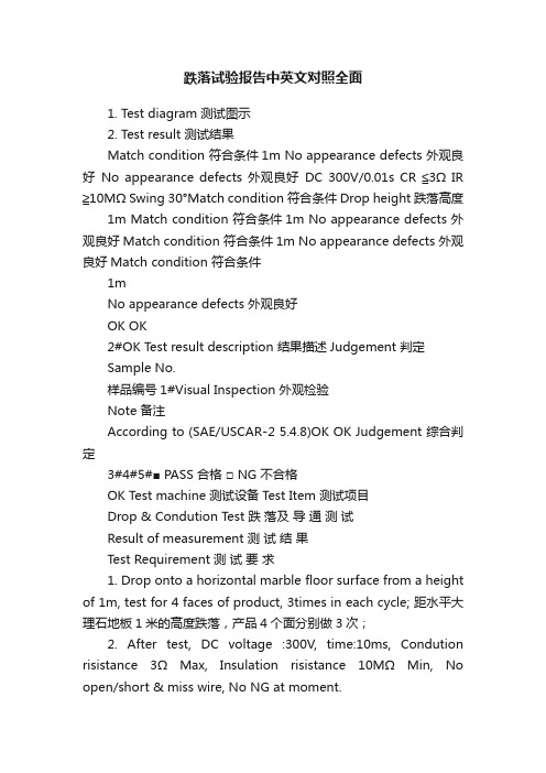
跌落试验报告中英文对照全面1. Test diagram 测试图示2. Test result 测试结果Match condition 符合条件1m No appearance defects 外观良好No appearance defects 外观良好DC 300V/0.01s CR ≦3Ω IR ≧10MΩ Swing 30°Match condition 符合条件Drop height 跌落高度1m Match condition 符合条件1m No appearance defects 外观良好Match condition 符合条件1m No appearance defects 外观良好Match condition 符合条件1mNo appearance defects 外观良好OK OK2#OK Test result description 结果描述Judgement 判定Sample No.样品编号1#Visual Inspection 外观检验Note 备注According to (SAE/USCAR-2 5.4.8)OK OK Judgement 综合判定3#4#5#■ PASS 合格□ NG 不合格OK Test machine 测试设备Test Item 测试项目Drop & Condution Test 跌落及导通测试Result of measurement 测试结果Test Requirement 测试要求1. Drop onto a horizontal marble floor surface from a height of 1m, test for 4 faces of product, 3times in each cycle; 距水平大理石地板1米的高度跌落,产品4个面分别做3次;2. After test, DC voltage :300V, time:10ms, Condution risistance 3Ω Max, Insulation risistance 10MΩ Min, No open/short & miss wire, No NG at moment.试验后,DC 电压300V,持续时间10ms, 导通阻抗≦3Ω,绝缘阻抗≧10M Ω,无开路,短路和错接,无瞬间不良现象;3. Connect the cable to the test machine, when testing, Two-hands catch the cable swing up and down at 30 degree; 将线材与测试机连接,当测试时,两手抓住线材做上下30度的摇摆;4. After test, no appearance defects; 测试后外观良好;SHENZHEN EAST-TOPTECH ELECTRONIC TECHNOLOGY CO.,LTD深圳市东景盛电子技术有限公司Drop & Condution Test Report 跌落及导通测试报告Product name 样品名称Product spec.产品规格HDMI AM TO AM 30AWG 1.4REV. OD :5.0mm Length :1.5/2.0MCustomer 客户名称/Test date 测试日期5PCS/2014-9-22Marble Floor 大理石地板T est environment测试环境Drawing NO.工程图号HDMI M/M Ni Plated 30AWG OD:5.0 L=1.5/2.0M Black/Sample Q'ty 样品数量Part/No.产品料号温度:28℃/湿度:75%表单编号:DJS-QR-045。
不同提取方法对井冈蜜柚皮精油组成与性质的影响

李欣,华建新,罗杰洪,等. 不同提取方法对井冈蜜柚皮精油组成与性质的影响[J]. 食品工业科技,2024,45(3):83−97. doi:10.13386/j.issn1002-0306.2023030289LI Xin, HUA Jianxin, LUO Jiehong, et al. Effects of Different Extraction Methods on the Composition and Properties of Jinggang Pomelo Peel Essential Oil[J]. Science and Technology of Food Industry, 2024, 45(3): 83−97. (in Chinese with English abstract). doi:10.13386/j.issn1002-0306.2023030289· 研究与探讨 ·不同提取方法对井冈蜜柚皮精油组成与性质的影响李 欣1,华建新1,罗杰洪1,王国庆2,陈 赣2,周爱梅1,*(1.华南农业大学食品学院,广东省功能食品活性重点实验室,广东广州 510642;2.吉安井冈农业生物科技有限公司,江西吉安 343016)摘 要:以井冈蜜柚皮精油(Jinggang pomelo peel essential oil ,JPPEO )为研究对象,采用水蒸气蒸馏法、低温连续相变法两种方法进行提取,以精油得率为主要指标,研究了萃取温度、压力、时间等因素对井冈蜜柚皮精油得率的影响,并通过正交法进行低温连续相变法提取工艺优化,同时对精油的理化性质及化学组成进行分析。
研究表明,低温连续相变提取井冈蜜柚皮精油(Low-temperature continuous phase transition extraction essential oil ,L-JPPEO )的最佳工艺为:颗粒度30目,萃取温度55 ℃,萃取压力0.6 MPa ,萃取时间60 min ,解析温度70 ℃,此时精油得率为10.99‰,比水蒸气蒸馏法提取的精油(Hydro distillation essential oil ,H-JPPEO )得率高出了2.88倍;理化性质实验结果表明,低温连续相变萃取的井冈蜜柚皮精油的不饱和脂肪酸含量较高,游离脂肪酸含量较低,酯类成分含量较低;傅里叶衰减全反射中红外光谱法(Fourier transform infrared spectroscopy ,FTIR )鉴定出L-JPPEO 和H-JPPEO 含萜烯类化合物、醇类、酚类、醛类以及含羰基化合物。
EIA-364-28F_(2011-01-14)_Vibration

EIASTANDARDTP-28FVIBRATION TEST PROCEDURE FOR ELECTRICAL CONNECTORS AND SOCKETSEIA-364-28FJANUARY 2011EIA StandardsElectronic Components AssociationANSI/EIA-364-28F-2011Approved: January 14, 2011E I A -364-28FNOTICEThis standard is based upon the major technical content of International Electrotechnical Commission standard 60512-2-1 2005-Febuary (was IEC 512-2, test 2a), contact resistance - millivolt level method. It conforms in all essential respects this IEC standard.EIA Engineering Standards and Publications are designed to serve the public interest through eliminating misunderstandings between manufacturers and purchasers, facilitating interchangeability and improvement of products, and assisting the purchaser in selecting and obtaining with minimum delay the proper product for his particular need. Existence of such Standards and Publications shall not in any respect preclude any member or nonmember of ECA from manufacturing or selling products not conforming to such Standards and Publications, nor shall the existence of such Standards and Publications preclude their voluntary use by those other than ECA members, whether the standard is to be used either domestically or internationally.Standards and Publications are adopted by ECA in accordance with the American National Standards Institute (ANSI) patent policy. By such action, ECA does not assume any liability to any patent owner, nor does it assume any obligation whatever to parties adopting the Standard or Publication.This major portion of this Standard is based upon the technical content of International Electrotechnical Commission standard IEC 60512-6-4, (was IEC 512-4, test 6d) Dynamic Stress, Vibration (Sinusoidal), 2002 and also IEC 60512-6-5, Dynamic Stress, Random Vibration, 1997. It differs from IEC Publication 60068-2-6 (was IEC 68-2-6, test Fc), Vibration (Sinusoidal), 2007; by specifying a single test with closely controlled conditions and methods for random vibration. These differences have been called to the attention of the U.S. Committee of Experts for IEC (or ISO) Technical Committee TC48 and resolution of these differences will be sought in future meetings of SC48. Test condition VII is based on International Electrotechnical Commission standard IEC 60068-2-34, (was IEC 68-2-34, Test Fd), Random Vibration Wide Band, 1993.This Standard does not purport to address all safety problems associated with its use or all applicable regulatory requirements. It is the responsibility of the user of this Standard to establish appropriate safety and health practices and to determine the applicability of regulatory limitations before its use.(From Standards Proposal No. SP-5212 formulated under the cognizance of the CE-2.0 National Connector Standards Committee).Published by©ELECTRONIC COMPONENTS ASSOCIATION 2011Engineering Department2500 Wilson Boulevard, Suite 310Arlington, VA 22201PRICE: Please call: IHSUSA and Canada (1-800-854-7179)All rights reservedPrinted in U.S.A.PLEASE!DON'T VIOLATETHELAW!This document is copyrighted by the ECA and may not be reproduced without permission.Organizations may obtain permission to reproduce a limited number of copies through entering into a license agreement. For information, contact:IHS15 Inverness Way EastEnglewood, CO 80112-5704 or callUSA and Canada (1-800-854-7179), International (303-397-7956)CONTENTSClause Page 1 Introduction (1)1.1 Scope (1)1.2 Object (1)1.3 Applicable documents (1)1.4 Definitions (1)2 Test resources (2)2.1 Equipment (2)3 Test specimen (3)4 Test procedure (4)4.1 Test conditions I, II, III and IV (4)4.2 Test conditions V, VI and VII (10)5 Details to be specified (16)6 Test documentation (17)Table1 Vibration conditions (4)2 Values for test condition V (13)3 Values for test condition VI (14)4 Values for test condition VII (15)Figure1 Mounting axis definitions (2)2 Vibration test curves - high frequency (displacement in mm) (6)3 Vibration test curves - high frequency (displacement in inches) (7)4 Test condition V, random vibration test curve envelope (13)5 Test condition VI, random vibration test curve envelope (14)6 Test condition VII, random vibration test curve envelope (15)(This page left blank)TEST PROCEDURE No. 28FVIBRATION TEST PROCEDUREFORELECTRICAL CONNECTORS AND SOCKETS(From EIA Standards Proposal No. 5212, formulated under the cognizance EIA CE-2.0 Committee on National Connector Standards, and previously published in EIA-364-28E.)1 Introduction1.1 ScopeThe standard test procedure details a method to assess the ability of electrical connector components to withstand specified severities of vibration.1.2 ObjectThe object of this test is to determine the effects of vibration within the predominant or random vibration frequency ranges and magnitudes that may be encountered during the life of the connector.1.3 Applicable documentsThe following documents form a part of this standard to the extent indicated herein. In the event of conflict between the requirements of this standard and the referenced documents, this standard takes precedence.1.3.1 EIA standardsEIA-364-46: Microsecond Discontinuity Test Procedure for Electrical Connectors, Contacts and SocketsEIA-364-87: Nanosecond Event Detection for Electrical Connectors, Contacts and Sockets1.4 Definitions1.4.1 AxisThe following mounting axis definitions shall be employed during the performance of this test. Figure 1 indicates a pictorial view of the axis definitions. The referencing document shall indicate the fixturing required or the axis definitions if different than as stated in figure 1. Axis definitions for symmetrical, square and “free” connectors shall be defined in the Detail Specification.1.4.1.1 X-axisAlong the longitudinal length of the test sample1.4.1.2 Y-axisThe axis perpendicular to the longitudinal length of the sample (transverse direction).1.4.1.3 Z-axisThe axis perpendicular to the fixture seating plane attached to the test table.Figure 1 - Mounting axis definitions1.4.2 The term gnThis term is the SI unit for the standard acceleration due to the earth’s gravity, which itself varies with altitude and geographic latitude. NOTE — In this standard the value of g n is 9.81 m/s 2.2. Test resources2.1 Equipment2.1.1 The monitoring transducer shall be calibrated against a standard transducer having an accuracy of ±2%. The vibration system consisting of the vibration machine, together with its auxiliary test equipment, shall be capable of generating either a sinusoidal or random excitation.2.1.2 Test equipment for random vibration shall produce random excitation that possesses a gaussian (normal) amplitude distribution, except that the acceleration magnitudes of the peak values may be limited to a minimum of three times the rms [three-sigma (3σ) limits].3 Test specimen3.1 A vibration test sample shall be a fully wired connector consisting of one of the following, as applicable;3.1.1 A connector plug and its mating connector receptacle.3.1.2 A printed circuit connector receptacle and its mating connector board(s).3.1.3 An integral, functional connector assembly.3.2 Each test sample shall be prepared with wire and other materials or processes, simulating application assembly of the sample. If normal connector mating is dependent upon forces external to the connector, then such forces and mounting arrangement shall be as closely duplicated as possible (example: printed circuit connectors). If mating is achieved with normal locking means, then only normal locking means shall be used.3.3 Method of mounting3.3.1 Test conditions I, II, III and IV (sinusoidal evaluation conditions)The specimen shall be attached to a fixture capable of transmitting the vibration conditions specified. The test fixture shall be designed so that resonant vibration inherent in the fixture within the frequency range specified for the test shall be minor. The magnitude of the applied vibration shall be monitored on the test fixture near the specimen mounting points. The test specimen shall be mounted rigidly to the test fixture as specified and shall simulate as closely as possible the normal mounting of the specimen. A minimum of 200 mm (approx 8 in) of wire or cable shall be unsupported on both ends of the connector. For specimens with attached brackets, one of the vibration-test directions shall be parallel to the mounting surface of the bracket. Vibration input shall be monitored on the mounting fixture in the proximity of the support points of the specimen.3.3.2 Test conditions V, VI and VII (random excitation conditions)The specimen shall be mounted as specified. The orientation of the specimen or direction of application of the applied vibration motion shall be specified in one or more directions. If the order of application of the different directions is critical, it also shall be specified. Any special test fixtures or jigs required to run the test shall be specified in sufficient detail to assure reproducibility of the input motion applied to the specimen. These details shall include the dimensions, the materials, temper, etc., as applicable.4 Test procedureTests and measurements before, during and after vibration shall be as specified in the referencing document.4.1 Test conditions I, II, III and IV4.1.1 Electrical load and discontinuity4.1.1.1 Unless otherwise specified in the referencing document, an electrical load of 100 milliamperes maximum with a detector capable of detecting a discontinuity of 1.0 microsecond or longer. Said monitoring shall be performed in accordance with EIA-.364-46.4.1.1.2 Unless otherwise specified in the referencing document, low nanosecond event detection shall be performed in accordance with EIA-364-87. A 100 milliamperes test current shall be applied to the areas being monitored. A detector capable of measuring an event resulting in a 10 ohm change lasting longer than 10 nanoseconds, unless otherwise specified in the referencing document.4.1.1.2.1 Low nanosecond event detection shall not be used as a substitute for the standard 1.0 microsecond requirement. This monitoring test was developed to detect different failure mechanisms than that described in 4.1.1.1. It is designed to detect large resistance fluctuations or voltage variations that may result in improper triggering of high speed digital circuits.4.1.2 Vibration conditionsVibration conditions shall be in accordance with table 1, as applicable.Table 1 - Vibration conditionsTest conditions Frequency range, Hz Peak levelg n m/s2I Low - 10 to 55II High - 10 to 500 10 98.1III High - 10 to 2,000 15 147.1IV High - 10 to 2,000 20 196.14.1.3 ResonanceA critical resonant frequency is that frequency at which any point on the specimen is observed to have a maximum amplitude more than twice that of the support points. When specified, resonant frequencies shall be determined either by monitoring parameters such as contact opening, or by use of resonance-detecting instrumentation.4.1.4 Test condition IThe specimens shall be subjected to a simple harmonic motion having an amplitude 1.52 mm (0.06 in) double amplitude (maximum total excursion), the frequency being varied uniformly between the approximate limits of 10 Hz and 55 Hz. The entire frequency range, from 10 Hz to 55 Hz and return to 10 Hz, shall be traversed in approximately 1 minute. Unless otherwise specified, this motion shall be applied for 2 hours in each of three mutually perpendicular directions (total of 6 hours). If applicable, this test shall be made under electrical load conditions.4.1.5 Test condition II [98.1 m/s2 (10 g n) peak]The specimens, while deenergized or operating under the load conditions specified, shall be subjected to the vibration amplitude, frequency range, and duration specified 4.1.5.1, 4.1.5.2 and 4.1.5.3, respectively; see figures 2 and 3.4.1.5.1 AmplitudeThe specimens shall be subjected to a simple harmonic motion having an amplitude of either 1.52 mm (0.06 in) double amplitude (maximum total excursion) or 98.1 m/s2(10 g n) peak, whichever is less. The tolerance on vibration amplitude shall be ±10%.4.1.5.2 FrequencyThe vibration frequency shall be varied logarithmically between the approximate limits of 10 Hz and 500 Hz (see 4.1.8) except that the procedure (see 4.1.4) of this standard may be applied during the 10 Hz to 55 Hz band of the vibration frequency range.4.1.5.3 Sweep time and durationThe entire frequency range of 10 Hz to 500 Hz and return to 10 Hz shall be traversed in 15 minutes. This cycle shall be performed 12 times in each of three mutually perpendicular directions (total of 36 times), so that the motion shall be applied for a total period of approximately 9 hours. Interruptions are permitted provided the requirements for rate of change and test duration are met. Completion of cycling within any separate band is permissible before going to the next band. When the procedure (see 4.1.4) is used for the 10 Hz to 55 Hz band, the duration of this portion shall be same as the duration for this band using logarithmic cycling (approximately 1-1/3 hours in each of three mutually perpendicular directions).4.1.6 Test condition III 147.1 m/s2 (15 g n) peak]The specimens, while deenergized or operating under the load conditions specified, shall be subjected to the vibration amplitude, frequency range, and duration specified in 4.1.6.1, 4.1.6.2 and 4.1.6.3, respectively; see figures 2 and 3.NOTE: g = 0.00201f 2 DA (f = frequency in hertz, DA = double amplitude in mm)Figure 2 - Vibration test curves - high frequency (displacement in mm)NOTE: g = 0.0512f 2 DA (f = frequency in hertz, DA = double amplitude in inches) Figure 3 - Vibration test curves - high frequency (displacement in inches)4.1.6.1 AmplitudeThe specimens shall be subjected to a simple harmonic motion having an amplitude of either 1.52 mm (0.06 in) double amplitude (maximum total excursion) or 147.1 m/s2(15 g n) peak, whichever is less. The tolerance on vibration amplitude shall be ±10%.4.1.6.2 Frequency rangeThe vibration frequency shall be varied logarithmically between the approximate limits of 10 Hz to 2,000 Hz (see 4.1.8) except that the procedure (see 4.1.4) of this standard may be applied during the 10 Hz to 55 Hz band of the vibration frequency range.4.1.6.3 Sweep time and durationThe entire frequency range of 10 Hz to 2,000 Hz and return to 10 Hz shall be traversed in 20 minutes. This cycle shall be performed 12 times in each of three mutually perpendicular directions (total of 36 times), so that the motion shall be applied for a total period of approximately 12 hours. Interruptions are permitted provided the requirements for rate of change and test duration are met. Completion of cycling within any separate band is permissible before going to the next band. When the procedure (see 4.1.4) of this standard is used for the 10 Hz to 55 Hz band, the duration of this portion shall be the same as the duration for this band using logarithmic cycling (approximately 1-1/3 hours in each of three mutually perpendicular directions).4.1.7 Test condition IV [196.1 m/s2 (20 g n) peak]The specimens, while deenergized or operating under the load conditions specified, shall be subjected to the vibration amplitude, frequency range, and duration specified in 4.1.7.1, 4.1.7.2 and 4.1.7.3, respectively; see figures 2 and 3.4.1.7.1 AmplitudeThe specimens shall be subjected to a simple harmonic motion having an amplitude of either 1.52 mm (0.06 in) double amplitude (maximum total excursion) or 196.1 m/s2(20 g n) peak, whichever is less. The tolerance on vibration amplitude shall be ±10%.4.1.7.2 Frequency rangeThe vibration frequency shall be varied logarithmically between the approximate limits of 10 Hz to 2,000 Hz (see 4.1.8).4.1.7.3 Sweep time and durationThe entire frequency range of 10 Hz to 2,000 Hz and return to 10 Hz shall be traversed in 20 minutes. This cycle shall be performed 12 times in each of three mutually perpendicular directions (total of 36 times), so that the motion shall be applied for a total period of approximately 12 hours. Interruptions are permitted provided the requirements for rate of change and test duration are met.Completion of cycling within any separate band is permissible before going to the next band. When the procedure (see 4.1.4.) of this standard is used for the 10 Hz to 55 Hz band, the duration of this portion shall be the same as the duration for this band using logarithmic cycling (approximately 1-1/3 hours in each of three mutually perpendicular directions).4.1.8 Alternative procedure for use of linear in place of logarithmic change of frequency Linear rate of change of frequency is permissible under the following conditions:4.1.8.1 The frequency range above 55 Hz shall be subdivided into no fewer than three bands. The ratio of the maximum frequency to the minimum frequency in each band shall be not less than two (2).4.1.8.2 The rate of change of frequency in Hz per minute shall be constant within any one band.4.1.8.3 The ratios of the rate of change of frequency of each band to the maximum frequency of that band shall be approximately equal.4.1.8.3.1 Example of alternative procedureAs an example of the computation of rates of change, assume that the frequency spectrum has been divided into three bands, 55 Hz to 125 Hz, 125 Hz to 500 Hz and 500 Hz to 2,000 Hz, in accordance with 4.1.8.1. For each band, let the constant, κ, represent the frequency change (in Hz/minute), divided by the maximum frequency (in Hz). Then the rates of change for the three bands will be 125κ, 500κ and 2,000κ, respectively. The times (in minutes) to traverse the three frequency bands are1255512550012550020005002000−−−κκκ,,,andSince the minimum total sweep time is 30 minutes,701253755001500200030κκκ++=,,whence κ = 0.0687/minute.The required maximum constant rates of frequency change for the three bands are therefore 8.55 Hz per minute, 34.2 Hz per minute and 137 Hz per minute, respectively. The minimum times of traverse of the bands are 8.2 min, 10.9 min and 10.9 min, respectively.4.2 Test conditions V, VI and VII4.2.1 Control and analysis of random vibration4.2.1.1 Spectral density curvesThe output of the vibration machine shall be presented graphically as power-spectral density versus frequency; see 4.2.1.1.1. The spectral-density values shall be within +40% and -30% (±1.5 dB) of the specified values between a lower-specified frequency and 1,000 Hz, and within +100% and -50% (±3 dB) of the specified values between 1,000 and an upper-specified frequency (2,000 Hz). A filter bandwidth will be a maximum of 1/3-octave or a frequency of 25 Hz, whichever is greater.4.2.1.1.1 Power-spectral densityPower-spectral density is the mean-square value of an oscillation passed by a narrow-band filter per unit-filter bandwidth. For this application it is expressed as g 2 / f, where g 2 / f is the mean-square value of acceleration expressed in gravitational units per number of cycles of filter bandwidth. The spectral density curves are usually plotted either on a logarithmic scale, or in units of decibels (dB). The number of decibels is defined by the equation:The rms value of acceleration within a frequency band between f 1 and f 2 is:g = f df rms 2f f 12g ∫//12where g r 2 / f is a given reference value of power-spectral density, usually the maximum specified value.4.2.1.2 Distribution curvesA probability density-distribution curve may be obtained and compared with a gaussian-distribution curve. The experimentally-obtained curve shall not differ from the gaussian curve by more than ± 10% of the maximum value.4.2.1.3 MonitoringMonitoring involves measurements of the vibration excitation and of the test item performance. When required in the referencing document, the specimen may be monitored during the test. The details of the monitoring circuit, including the method and points of connection to the specimen, shall be specified.dB = 10 g /f g /f = 20 g /fg /f2r r log log 24.2.1.4 Vibration inputThe vibration magnitude shall be monitored on a vibration machine, on mounting fixtures, at locations that are as near as practicable to the test item mounting points. When the vibration input is measured at more than one point, the minimum input vibration shall normally be made to correspond to the specified test curve; see figures 4 and 5. For massive test items and fixtures, and for large force exciters or multiple vibration exciters, the input control value may be an average of the average magnitudes of three or more inputs. Accelerations in the transverse direction, measured at the test item attachment points, shall be limited to 100% of the applied vibration. The number and location of the test points shall be specified.4.2.2 ProcedureThe specimen, or substitute equivalent mass, shall be mounted in accordance with 3.3.2 and the monitoring equipment attached, if applicable, in accordance with 4.2.1.3. The vibration machine shall then be operated and equalized or compensated to deliver the required frequencies and intensities conforming to the curves specified in test condition V, figure 4, or test condition VI, figure 5, or test condition VII, figure 6 (see 2.1). The specimen shall then be subjected to the vibration specified by the test condition letter (see tables 2, 3 and 4) for the duration as specified:3 minutes; 15 minutes; 1-1/2 hours; or 8 hours;in each of three mutually perpendicular directions, and in the order specified (see 3.3.2), as applicable.The measurements made before, during, and after the test shall be specified and if the specimen is to be monitored during the test, the details shall be in accordance with 4.2.1.3.4.2.3 Electrical load and discontinuities4.2.3.1 Unless otherwise specified in the referencing document, an electrical load of 100 milliamperes maximum with a detector capable of detecting a discontinuity of 1.0 microsecond or longer. Said monitoring shall be performed in accordance with EIA-.364-46.4.2.3.2 Unless otherwise specified in the referencing document, low nanosecond event detection shall be performed in accordance with EIA-364-87. A 100 milliamperes test current shall be applied to the areas being monitored. A detector capable of measuring an event resulting in a 10 ohm change lasting longer than 10 nanoseconds, unless otherwise specified in the referencing document.4.2.3.2.1 Low nanosecond event detection shall not be used as a substitute for the standard 1.0 microsecond requirement. This monitoring test was developed to detect different failure mechanisms than that described in 4.2.3.1. It is designed to detect large resistance fluctuations or voltage variations that may result in improper triggering of high speed digital circuits.Figure 4 - Test condition V, random vibration test-curve envelope (see table 2).Table 2 - Values for test condition V 1)Test condition letter Power spectral density, g 2/Hz Overall rms gA 0.02 5.35B 0.04 7.56C 0.06 9.26D 0.1 11.95E 0.2 16.91F 0.3 20.71G 0.4 23.91H 0.6 29.28I Superseded by Test condition letterJ J 1.0 37.80K 1.5 46.301) For duration of test; see 4.2.2.Figure 5 - Test condition VI, random vibration test-curve envelope (see table 3).Table 3 - Values for test-condition VI 1)Test condition letter Power spectral density, g 2/Hz Overall rms gA 0.02 6.21B 0.04 8.78C 0.06 10.76D 0.1 13.89E 0.2 19.64F 0.3 24.06G 0.4 27.78H 0.6 34.02I Superseded by Test condition letterJ J 1.0 43.92K 1.5 53.791) For duration of test; see 4.2.2.Figure 6 - Test condition VII, random vibration test-curve envelope (see table 4)Table 4 - Values for test condition VII 1)Test condition letter Power spectraldensity, g 2/Hz Overall rms gA 0.002 0.98B 0.005 1.55C 0.01 2.19D 0.02 3.10E 0.05 4.90F 0.1 6.93G 0.29.801) For duration of test; see 4.2.2.5 Details to be specifiedThe following details shall be specified in the referencing document:5.1 Type of sample; see 3.15.2 Number of samples to be tested5.3 Method of mounting; see 3.35.4 Test condition number; see tables 1, 2, 3 or 45.5 Electrical load conditions, all contacts, if other than 100 milliamperes maximum; see 4.1.1 or 4.2.35.6 Discontinuity requirement if other than 1 microsecond5.7 Measurement of discontinuities during vibration; see 4.1.1 or 4.2.35.8 Method of determining resonance, if applicable; see 4.1.35.9 Direction of motion and order, if critical; see 3.35.10 Tests or measurements before, during and after vibration; see clause 45.11 Duration of vibration; see 4.1.4 or 4.2.25.12 Monitoring instrumentation, if applicable; see 4.2.1.35.13 Number and location of test points, if applicable; see 4.2.1.35.14 Mounting axes definitions if other than indicated in figure 1; see 1.46 Test documentationDocumentation shall contain the details specified in clause 5, with any exceptions, and the following:6.1 Title of test6.2 Sample description include fixture, if applicable6.3 Test equipment used, and date of last and next calibration6.4 Photographs, plots, values and observations necessary for proof of conformance6.5 Name of operator and start/finish date(s) of testRevision HistoryRevision letter ProjectnumberAdditions, changes and deletionsE SP-5125 Changed test condition letter I to J. Superseded testcondition letter I by J in table 2 and 3.F SP-5212 Add paragraph 1.3.Revise paragraph 4.1.1 and 4.2.3.EIA Document Improvement ProposalIf in the review or use of this document, a potential change is made evident for safety, health or technical reasons, please fill in the appropriate information below and mail or FAX to:Electronic Components AssociationEngineering Department2500 Wilson Blvd, Suite 310.Arlington, VA 22201FAX: (703-875-8908)Document No.: Document Title:Submitter’s Name: Telephone No.:FAX No.:e-mail:Address:Urgency of Change:Immediate: At next revision:Problem Area:a. Clause Number and /or Drawing:b. Recommended Changes:c. Reason/Rationale for Recommendation:Additional Remarks:Signature: Date:2FOR ECA USE ONLYResponsible Committee:Chairman:Date comments forwarded to Committee Chairman:Electronic Components Association2500 Wilson Boulevard, Suite 310 * Arlington, VA 22201 * tel 703-907-8021 * fax 703-875-8908。
条件空气机使用说明书

123456Emptying condensationAfter each drying cycle, empty the condensate container; otherwise the next drying programme may be cancelled as a result of the condensate container being full.1.Pull out condensate container keeping it horizontal.2.Pour out condensation.3.Always push container in fully until it clicks into place.If Í Container flashes in the display panel a What to do if..., Page 10.Cleaning the fluff filterClean the fluff filter after each drying operation.1.Open the door, remove fluff from door/door area.2.Pull out and fold open the fluff filter.3.Remove the fluff (by wiping the filter with your hand).If the fluff filter is very dirty or blocked, rinse with warm water and dry thoroughly.4.Close and reinsert the fluff filter.Switching off the dryerTurn the programme selector to Off .Do not leave laundry in the dryer.Removing the laundryThe automatic anti-crease function causes the drum to move at specific intervals, the washing remains loose and fluffy for an hour (two hours if the additional S Reduced Ironing function is also selected-depending on model ).... and adapt to individualNever start the dryer if it is damaged!Inform your after-sales service.Inspecting thedryer Sorting and loading laundryRemove all items from pockets.Check for cigarette lighters.The drum must be empty prior to loading.See programme overview on page 7.See also separate instructions for “Woollens basket” (depending on model)Your new dryerCongratulations - You have chosen a modern, high-quality Bosch Intended usePreparing for installation, see Page 8Selecting and adjusting the programmeDryingCondensate container Control panelʋfor domestic use only,ʋonly to be used for drying fabrics that have beenwashed with water.Keep children younger than 3 years old away from the dryer.Do not let children make the cleaning andmaintenance work on the dryer without supervision.Do not leave children unsupervised near the dryer.Keep pets away from the dryer.The dryer can be operated by children 8 years old and older, by persons with reduced physical, sensory or mental abilities and by persons with insufficient experience or knowledge if they are supervised or have been instructed in its use by a responsible adult.This appliance is intended for use up to a maximum height of 4000 metres above sea level.Select the drying programme ...123Make sure your hands are dry. Hold the plug only.Connecting themains plugDryingInformation on laundry ...Labelling of fabricsFollow the manufacturer's care information.(c Drying at normal temperature.'c Drying at low temperature a also select V Low Heat .)c Do not machine dry.Observe safety instructions without fail a Page 11!Do not tumble-dry the following fabrics for example:–Impermeable fabrics (e.g. rubber-coated fabrics).–Delicate materials (silk or curtains made from synthetic material) a they may crease.–Laundry contaminated with oil.Drying tips–To ensure a consistent result, sort the laundry by fabric type and drying programme.–Always dry very small items (e.g. baby socks) together with large items of laundry (e.g. hand towel).–Close zips, hooks and eyelets, and button up covers. Tie fabric belts, apron strings, etc. together.–Do not over-dry easy-care laundry a risk of creasing! Allow laundry to finish drying in the air.–Do not dry woolens in the dryer, only use to freshen them up a Page 7, Woollens finish Programme (depending on model).–Do not iron laundry immediately after drying, fold items up and leave for a while a the remaining moisture will then be distributed evenly.–The drying result depends on the type of water used during washing. a Fine adjustment of the drying result a Page 5/6.–Machine-knitted fabrics (e.g. T-shirts or jerseys) often shrink the first time they are dried a do not use the Cupboard Dry Plus programme.–Starched laundry is not always suitable for dryers a starch leaves behind a coating that adversely affects the drying operation.–Use the correct dosage of fabric softener as per the manufacturer's instructions when washing the laundry to be dried.–Use the timer programme for small loads a this improves the drying result.Environmental protection / Energy-saving tips–Before drying, spin the laundry thoroughly in the washing machine a the higher the spin speed the shorter the drying time will be (consumes less energy), also spin easy-care laundry.–Put in, but do not exceed, the maximum recommended quantity of laundry a programme overview a Page 7.–Make sure the room is well ventilated during drying.–Do not obstruct or seal up the air inlet.–Keep the air cooler clean a Page 6 “Care and cleaning”.Fine adjustment of the drying resultAdjustment of the levels of dryness1 x to the rightPress and hold V Low Heat and turn 5 x to the rightPress V Low Heat until the required level is reached Turn to OffTurn to OffDrumAll buttons are sensitive and only need to be touched lightly.Only operate the dryerAir inletFluff filterDrum interior light (depending on model)Maintenance flapProgramme end once lights up in the display. Interrupt programme removing or adding laundry.The drying cycle can be interrupted for a brief period so that laundry may be added or removed. The programme selected must then be resumed and completed.Never switch the dryer off before the drying process has ended.Drum and door may be hot!1.Open door, the drying process is interrupted.2.Load or remove laundry and close door.3.If required, select a new programme and additional functions.4.Press the Start/Stop button.Programme selectorDisplay panelService indicatorsÍ Container n FilterClean the fluff filter and/or air cooler under running water. a Page 4/6.Fineadjustment of the drying resultThe drying result (e.g. Cupboard Dry) can be adjusted over three levels (1 - max. 3) and A Super Quick 40’ programmes a presetting = 0. After one of these programmes has been finely adjusted, the setting is retained for the Page 5/6.0, 1, 2, 3 Fine adjustment of the drying resultCare and cleaningDryer housing, control panel, air cooler, moisture sensors–Wipe with a soft, damp cloth.–Do not use harsh cleaning agents and solvents.–Remove detergent and cleaning agent residue immediately.Clean the protective filter 5 - 6 times a year or if n Filter flashes after cleaning the fluff filter.Air cooler / Protective filterWhen cleaning, only remove the protective filter. Clean the air cooler behind the protective filter once a year.–Allow the dryer to cool.–Residual water may leak out, so place an absorbent towel underneath the maintenance door.1.Unlock the maintenance door.2.Open the maintenance door fully.3.Turn both locking levers towards each another.4.Pull out the protective filter/air cooler.Do not damage the protective filter or air cooler.Clean with warm water only. Do not use any hard or sharp-edged objects.5.Clean the protective filter/air cooler thoroughly,Allow to drip dry.6.Clean the seals.7.Re-insert the protective filter/air cooler,with the handle facing down.8.Turn back both locking levers.9.Close the maintenance door until the lock clicks into place.Moisture sensorsThe dryer is fitted with stainless steel moisture sensors. The sensors measure the level of moisture in the laundry. After a long period of operation, a fine layer of limescale may form on the sensors.1.Open the door and clean the moisture sensors with a damp spongewhich has a rough surface.Do not use steel wool or abrasive materials.Drying H , Iron Dry |, Cupboard Dry +,Anti-crease/End R / are displayed in sequence.Short signal when changing from level 3 to 0, otherwise long signal.Only when switched off!Press the Start/Stop button*D r y n e s s l e v e l s c a n b e s e l e c t e d i n d i v i d u a l l y a C u p b o a r d D r y P l u s ,c + C u p b o a r d D r y a n d | I r o n D r y (d e p e n d i n g o n t h e m o d e l ).D e g r e e o f d r y n e s s c a n b e f i n e l y a d j u s t e d ; m u l t i -l a y e r e d t e x t i l e s r e q u i r e a l o n g e r d r y i n g t i m e t h a n s i n g l e -l a y e r e d i t e m s o f c l o t h i n g . R e c o m m e n d a t i o n : D r y s e p a r a t e l y .Page 11.Connect to an AC earthed socket. If in doubt have the socket checked by an expert.The mains voltage and the voltage shown on the rating plate (a Page 9) must correspond.The connected load and necessary fuse protection are specified on the rating plate.Note the fuse protection of the socket.The values for the energy label are determined using a circuit breaker/fuse rating of 16 A. If the circuit breaker/fuse rating is changed to 10 A, the drying time and energy consumption will be higher. You can find details on this in the consumption values table. a Page 9Make sure that the air inlet remains unobstructedClean and levelpress and hold selection then turn 3 x to the right turn to Offsetamperage off flashesDo not operate the dryer if there is a danger of frost.en Instruction manualDryerWTE84106ZA12Remove all items from pockets.Check for cigarette lighters.The drum must be empty prior to loading.See programme overview on page 7.See also separate instructions for “Woollens ba (depending on model)domestic appliance.The condensation dryer is distinguished by its economical energy consumption.Every dryer which leaves our factory is carefully checked to ensure that it functions correctly and is in perfect condition.Should you have any questions, our after-sales service will be pleased to help.Disposal in an environmentally-responsible manner This appliance is labelled in accordance with European Directive 2012/19/EU concerning used electrical and electronic appliances (waste electrical and electronic equipment - WEEE). The guideline determines the framework for the return and recycling of used appliances as applicable throughout the EU.For further information about our products, accessories, spare parts and services, please visit: All buttons are need to be touProgramme selector34Emptying condensationAfter each drying cycle, empty the condensate container; otherwise the next drying programme may be cancelled as a result of the condensate container being full.1.Pull out condensate container keeping it horizontal.2.Pour out condensation.3.Always push container in fully until it clicks into place.If Í Container flashes in the display panel a What to do if..., Page 10.Cleaning the fluff filterClean the fluff filter after each drying operation.1.Open the door, remove fluff from door/door area.2.Pull out and fold open the fluff filter.3.Remove the fluff (by wiping the filter with your hand).If the fluff filter is very dirty or blocked, rinse with warm water and dry thoroughly.4.Close and reinsert the fluff filter.Switching off the dryerTurn the programme selector to Off .Do not leave laundry in the dryer.Removing the laundryThe automatic anti-crease function causes the drum to move at specific intervals, the washing remains loose and fluffy for an hour (two hours if the additional S Reduced Ironing function is also selected-depending on model ).adapt to individualspecting thedryeroading laundryasket”he programmeDryingCondensate container Control paneldrying programme ...123nnecting the mains plugDryingDrume sensitive and only uched lightly.Air inletFluff filterDrum interior light (depending on model)Maintenance flapProgramme end once lights up in the display. Interrupt programme removing or adding laundry.The drying cycle can be interrupted for a brief period so that laundry may be added or removed. The programme selected must then be resumed and completed.Never switch the dryer off before the drying process has ended.Drum and door may be hot!1.Open door, the drying process is interrupted.2.Load or remove laundry and close door.Start/Stop buttonInformation on laundry ...Labelling of fabricsFollow the manufacturer's care information.(c Drying at normal temperature.'c Drying at low temperature a also select V Low Heat.)c Do not machine dry.Observe safety instructions without fail a Page 11!Do not tumble-dry the following fabrics for example:–Impermeable fabrics (e.g. rubber-coated fabrics).–Delicate materials (silk or curtains made from synthetic material) a they may crease.–Laundry contaminated with oil.Drying tips–To ensure a consistent result, sort the laundry by fabric type and drying programme.–Always dry very small items (e.g. baby socks) together with large items of laundry(e.g. hand towel).–Close zips, hooks and eyelets, and button up covers. Tie fabric belts, apron strings, etc.together.–Do not over-dry easy-care laundry a risk of creasing! Allow laundry to finish drying inthe air.–Do not dry woolens in the dryer, only use to freshen them up a Page 7, Woollens finish Programme (depending on model).–Do not iron laundry immediately after drying, fold items up and leave for a whilea the remaining moisture will then be distributed evenly.–The drying result depends on the type of water used during washing. a Fine adjustment of the drying result a Page 5/6.–Machine-knitted fabrics (e.g. T-shirts or jerseys) often shrink the first time they are drieda do not use the Cupboard Dry Plus programme.–Starched laundry is not always suitable for dryers a starch leaves behind a coating that adversely affects the drying operation.–Use the correct dosage of fabric softener as per the manufacturer's instructions whenwashing the laundry to be dried.–Use the timer programme for small loads a this improves the drying result.Environmental protection / Energy-saving tips–Before drying, spin the laundry thoroughly in the washing machine a the higher the spin speed the shorter the drying time will be (consumes less energy), also spin easy-carelaundry.–Put in, but do not exceed, the maximum recommended quantity of laundry a programme overview a Page 7.–Make sure the room is well ventilated during drying.–Do not obstruct or seal up the air inlet.–Keep the air cooler clean a Page 6 “Care and cleaning”.Fine adjustment of the drying resultAdjustment of the levels of dryness1 x to the right Press and hold V Low Heatand turn 5 x to the right Press V Low Heat until the required level is reachedTurn to Off Turn toOffFine adjustment of the drying resultCare and cleaningDryer housing, control panel, air cooler, moisture sensors–Wipe with a soft, damp cloth.–Do not use harsh cleaning agents and solvents.–Remove detergent and cleaning agent residue immediately.Clean the protective filter 5 - 6 times a yearor if n Filter flashes after cleaning the fluff filter.Air cooler / Protective filterWhen cleaning, only remove the protective filter. Clean the air coolerbehind the protective filter once a year.–Allow the dryer to cool.–Residual water may leak out, so place an absorbent towelunderneath the maintenance door.1.Unlock the maintenance door.2.Open the maintenance door fully.3.Turn both locking levers towards each another.4.Pull out the protective filter/air cooler.Do not damage the protective filter or air cooler.Clean with warm water only. Do not use any hard or sharp-edgedobjects.5.Clean the protective filter/air cooler thoroughly,Allow to drip dry.6.Clean the seals.7.Re-insert the protective filter/air cooler,with the handle facing down.8.Turn back both locking levers.9.Close the maintenance door until the lock clicks into place.Moisture sensorsThe dryer is fitted with stainless steel moisture sensors. The sensorsmeasure the level of moisture in the laundry. After a long period ofoperation, a fine layer of limescale may form on the sensors.1.Open the door and clean the moisture sensors with a damp spongewhich has a rough surface.Do not use steel wool or abrasive materials.Drying H, Iron Dry |, Cupboard Dry +,Anti-crease/End R / are displayed in sequence.Short signal when changing from level 3 to 0,otherwise long signal.Only when switched off!56*D r y n e s s l e v e l s c a n b e s e l e c t e d i n d i v i d u a l l y a C u p b o a r d D r y P l u s ,c + C u p b o a r d D r y a n d | I r o n D r y (d e p e n d i n g o n t h e m o d e l ).D e g r e e o f d r y n e s s c a n b e f i n e l y a d j u s t e d ; m u l t i -l a y e r e d t e x t i l e s r e q u i r e a l o n g e r d r y i n g t i m e t h a n s i n g l e -l a y e r e d i t e m s o f c l o t h i n g . R e c o m m e n d a t i o n : D r y s e p a r a t e l y .Page 11.Connect to an AC earthed socket. If in doubt have the socket checked by an expert.The mains voltage and the voltage shown on the rating plate (a Page 9) must correspond.The connected load and necessary fuse protection are specified on the rating plate.Note the fuse protection of the socket. The values for the energy label are determined using a circuit breaker/fuse rating of 16 A. If the circuit breaker/fuse rating is changed to 10 A, the drying time and energy consumption will be higher. You can find details on this in the consumption values table. a Page 9Make sure that the air inlet remains unobstructedClean and levelpress and hold selection then turn 3 x to the right turn to Offsetamperage off flashesDo not operate the dryer if there is a danger of frost.en Instruction manualDryerWTE84106ZA。
input hysteresis的含义
14down vote accepted Let's say you detect a low-to-high transition at 2.5 V. A 100 mV hysteresis would mean that the low-to-high transition is detected at 2.55 V and the high-to-low transition is detected at 2.45 V, a 100 mV difference.Hysteresis is used to prevent several quickly successive changes if the input signal would contain some noise, for example. Thenoise could mean you cross the threshold of 2.5 V more than just once, which you don't want.A 100 mV hysteresis means that noise levels less than 100 mV won't influence the threshold passing. Which threshold applies depends on whether you go from low to high (then it's the higher threshold) or from high to low (then it's the lower one):editAnother way to illustrate hysteresis is through its transfer function , with the typical loop:As long as the input voltage remains below \$V_{T+}\$ the output is low, but if it exceeds this value the output switches to high (the up-going arrow). Then the output remains high as long as the input voltage stays above \$V_{T-}\$. When the input voltage drops below this threshold the output switches to a low level (the down-going arrow).Note: hysteresis can also be used for other purposes than increasing noise immunity. The inverter below has a hysteresis input (which makes it a Schmitt trigger, indicated by the symbol inside the inverter). This simple circuit is all you need to make an oscillator.Here's how it works. When it's switched on the capacitor's voltage is zero, so the output is high (it's an inverter!). The high output voltage starts charging the capacitor through R. When the voltage over the capacitor reaches the higher threshold the inverter sees this as a high voltage, and the output will go low. The capacitor will now discharge to the low output via R until the lower threshold is reached. The inverter will then again see this as a low voltage, and make the output high, so the capacitor starts to charge again, and the whole thing repeats.The frequency is determined by the capacitor's and resistor's value as given in the equations. The difference between the frequency for the normal HCMOS (HC) and the TTL-compatible (HCT) is because the threshold levels are different for both parts.。
光耦FAIRCHILD_H_HCPL0600和6N137
光耦FAIRCHILD_H_HCPL0600和6N137HIGH SPEED-10 MBit/sLOGIC GATE OPTOCOUPLERSHCPL-0600HCPL-0601DESCRIPTIONThe HCPL-0600/0601optocouplers consist of a 870 nm AlGaAS LED, optically coupled to a very high speed integrated photo-detector logic gate with a strobable output. The devices are housed in a compact small-outline package. This output features an open collector, thereby permitting wired OR outputs. The coupled parameters are guaranteed over the temperature range of -40°C to +85°C. A maximum input signal of 5 mA will provide a minimum output sink current of 13 mA (fan out of 8). An internal noiseA 0.1 μF bypass capacitor must be connected between pins8 and 5. (See note 1)HIGH SPEED-10 MBit/sLOGIC GATE OPTOCOUPLERS HCPL-0600HCPL-0601*6.3 mA is a guard banded value which allows for at least 20% CTR degradation. Initial input current threshold value is 5.0 mA or lessHIGH SPEED-10 MBit/sLOGIC GATE OPTOCOUPLERS HCPL-0600HCPL-0601ELECTRICAL CHARACTERISTICS (T A = -40°C to +85°C Unless otherwise speci?ed.)INDIVIDUAL COMPONENT CHARACTERISTICSParameter Test Conditions Symbol Min Typ**Max UnitEMITTER(I F = 10 mA)V F 1.8VInput Forward Voltage T A =25°C 1.75Input Reverse Breakdown Voltage (I R = 10 μA)B VR 5.0V Input Capacitance(V F = 0, f = 1 MHz)C IN60pF Input Diode T emperature Coef?cient(I F = 10 mA)?VF/?T A-1.4mV/°C DETECTORHigh Level Supply Current (V CC = 5.5 V, I F = 0 mA)(V E = 0.5 V)I CCH710mALow Level Supply Current (V CC = 5.5 V, I F = 10 mA)(V E = 0.5 V)I CCL913mALow Level Enable Current(V CC = 5.5 V, V E = 0.5 V)I EL-0.8-1.6mA High Level Enable Current(V CC = 5.5 V, V E = 2.0 V)I EH-0.6-1.6mA High Level Enable Voltage(V CC = 5.5 V, I F = 10 mA)V EH 2.0V Low Level Enable Voltage(V CC = 5.5 V, I F = 10 mA) (Note 2)V EL0.8VSWITCHING CHARACTERISTICS (T A = -40°C to +85°C, V CC = 5 V, I F = 7.5 mA Unless otherwise speci?ed.) AC Characteristics Test Conditions Device Symbol Min Typ Max UnitPropagation Delay Time to Output High Level(Note 3)(T A =25°C)All T PLH204575ns (R L = 350?, C L = 15 pF) (Fig. 12)100Propagation Delay Time to Output Low Level(Note 4)(T A =25°C)All T PHL254575ns (R L = 350?, C L = 15 pF) (Fig. 12)100Pulse Width Distortion(R L = 350?, C L = 15 pF) (Fig. 12)All|TPHL-T PLH|335nsOutput Rise Time (10-90%)(R L = 350?, C L = 15 pF) (Note 5) (Fig. 12)All t r50nsOutput Fall Time (90-10%)(R L = 350?, C L = 15 pF) (Note 6) (Fig. 12)All t f12nsEnable Propagation Delay Timeto Output High Level (I F = 7.5 mA, V EH = 3.5 V)(R L = 350?, C L = 15 pF)(Note 7) (Fig. 13)All t ELH20nsEnable Propagation Delay Timeto Output Low Level (I F = 7.5 mA, V EH = 3.5 V)(R L = 350?, C L = 15 pF)(Note 8) (Fig. 13)All t EHL20nsCommon ModeT ransient Immunity (at Output High Level)(R L = 350?) (T A =25°C)(I F = 0 mA, V OH (Min.) = 2.0 V)(Note 9)(Fig. 14)|V CM| = 10 V HCPL-0600|CM H|10,000V/μs|V CM| = 50 V HCPL-0601500010,000Common ModeT ransient Immunity (at Output Low Level)(R L = 350?) (T A =25°C)(I F = 7.5 mA, V OL (Max.) = 0.8 V)(Note 10)(Fig. 14)|V CM| = 10 V HCPL-0600|CM H|10,000V/μs|V CM| = 50 V HCPL-0601500010,000HCPL-0600HCPL-0601** All typical values are at V CC = 5 V , T A = 25°C1.The V CC supply to each optoisolator must be bypassed bya 0.1μF capacitor or larger. This can be either a ceramic or solidtantalum capacitor with good high frequency characteristic and should be connected as close as possible to the package V CC and GND pins of each device.2.Enable Input - No pull up resistor required as the device has an internal pull up resistor.3.t PLH - Propagation delay is measured from the 3.75 mA level on the HIGH to LOW transition of the input current pulse to the1.5V level on the LOW to HIGH transition of the output voltage pulse. 4.t PHL - Propagation delay is measured from the 3.75 mA level on the LOW to HIGH transition of the input current pulse to the1.5V level on the HIGH to LOW transition of the output voltage pulse.5. t r - Rise time is measured from the 90% to the 10% levels on the LOW to HIGH transition of the output pulse.6.t f - Fall time is measured from the 10% to the 90% levels on the HIGH to LOW transition of the output pulse.7.t ELH - Enable input propagation delay is measured from the 1.5V level on the HIGH to LOW transition of the input voltagepulseto the 1.5V level on the LOW to HIGH transition of the output voltage pulse.8.t EHL - Enable input propagation delay is measured from the 1.5V level on the LOW to HIGH transition of the input voltage pulseto the 1.5V level on the HIGH to LOW transition of the output voltage pulse.9.CM H - The maximum tolerable rate of rise of the common mode voltage to ensure the output will remain in the high state (i.e.,V OUT > 2.0 V). Measured in volts per microsecond (V/μs).10.CM L - The maximum tolerable rate of fall of the common mode voltage to ensure the output will remain in the low output state(i.e., V OUT < 0.8 V). Measured in volts per microsecond (V/μs).11.Device considered a two-terminal device: Pins 1,2,3 and 4 shorted together, and Pins 5,6,7 and 8 shorted together.TRANSFER CHARACTERISTICS (T A = -40°C to +85°C Unless otherwise speci?ed.)DC Characteristics Test ConditionsSymbol MinTyp**Max Unit High Level Output Current (V CC = 5.5 V , V O = 5.5 V)(I F = 250 μA, V E = 2.0 V) (Note 2)I OH 100μA Low Level Output Voltage (V CC = 5.5 V , I F = 5 mA)(V E = 2.0 V , I OL = 13 mA) (Note 2)V OL .350.6V Input Threshold Current(V CC = 5.5 V , V O = 0.6 V ,V E = 2.0 V , I OL = 13 mA)I FT35mAISOLATION CHARACTERISTICS (T A = -40°C to +85°C Unless otherwise speci?ed.)CharacteristicsTest ConditionsSymbolMinTyp**MaxUnitInput-OutputInsulation Leakage Current (Relative humidity = 45%)(T A = 25°C, t = 5 s)(V I-O = 3000 VDC)(Note 11)I I-O1.0*μAWithstand Insulation T est Voltage (R H < 50%, T A = 25°C)(Note 11) ( t = 1 min.)V ISO 2500V RMS Resistance (Input to Output)(V I-O = 500 V) (Note11)R I-O 1012?Capacitance (Input to Output)(f = 1 MHz) (Note 11)C I-O0.6pFNOTESHCPL-0600HCPL-0601 TYPICAL PERFORMANCE CURVESHCPL-0600HCPL-0601HCPL-0600HCPL-0601HCPL-0600HCPL-0601MARKING INFORMATIONDe?nitions1Fairchild logo2Device number3VDE mark (Note: Only appears on parts ordered with VDE option – See order entry table)4One digit year code, e.g., ‘3’5T wo digit work week ranging from ‘01’ to ‘53’6Assembly package codeHCPL-0600HCPL-0601LIFE SUPPORT POLICYFAIRCHILD’S PRODUCTS ARE NOT AUTHORIZED FOR USE AS CRITICAL COMPONENTS IN LIFE SUPPORT DEVICES OR SYSTEMS WITHOUT THE EXPRESS WRITTEN APPROVAL OF THE PRESIDENT OF FAIRCHILD SEMICONDUCTOR CORPORATION. As used herein:1.Life support devices or systems are devices or systemswhich, (a) are intended for surgical implant into the body, or(b) support or sustain life, and (c) whose failure to performwhen properly used in accordance with instructions for use provided in the labeling, can be reasonably expected to result in a significant injury of the user.2. A critical component in any component of a life supportdevice or system whose failure to perform can be reasonably expected to cause the failure of the life support device or system, or to affect its safety or effectiveness.DISCLAIMERFAIRCHILD SEMICONDUCTOR RESERVES THE RIGHT TO MAKE CHANGES WITHOUT FURTHER NOTICE TOANY PRODUCTS HEREIN TO IMPROVE RELIABILITY, FUNCTION OR DESIGN. FAIRCHILD DOES NOT ASSUME ANY LIABILITY ARISING OUT OF THE APPLICATION OR USE OF ANY PRODUCT OR CIRCUIT DESCRIBED HEREIN; NEITHER DOES IT CONVEY ANY LICENSE UNDER ITS PATENT RIGHTS, NOR THE RIGHTS OF OTHERS.HCPL-0600HCPL-0601。
跌落测试规范(中英文)
跌落测试规范Drop Test Procedure1.0 PURPOSE (目的) :1.1All products must pass the Package Drop Test and/or SingleUnit Drop test . The purpose of this test is to give a certain degree of confidence that the product under test can be shipped via regular shipping channels without sustaining any damage.1.1 所有产品都需经过包装落下测试或单一落下测试合格,这个测试的是给予一确实的角度,让产品能经由正常的运送管道运送而没有损害。
2.0 SCOPE (范围) :2.1This procedure can be used for all packaged products independent of their weight, size or content. Special attention should be paid to the type of product that is contained in the package as to the types of test that should be run prior to and after the test. For a complete test series to meet the corporate specification, the vibration test should be run first and the Package Compression and Cold Drop Test should be run after this test.2.1 这个程序能够使用在所有包装产品,而他们的重量、大小、容量互相独立,要特别注意产品的型式,包含他们测试前后的包装,对于一个完整测试顺序的共同规范,振动测试需在此之前测试。
Thermo Scientific MK.4 ESD和Latch-Up测试系统中文名说明书
The Thermo Scientific MK.4 ESD and Latch-Up Test System is a complete,robust and feature-filled turn-key instrumentation test package, which performs automatic and manual HBM, MM, and Latch-Up tests on devices with pin counts up to 2304. It features the highest speed of test execution, lowest zap interval, and extensive parallelism that enables concurrent zapping with interleaved trace test capability to global and company driven quality standards.• Rapid-relay-based operations—up to 2304 channels• Solid state matrix topology for rapid, easy-to-use testing operations • Latch-Up stimulus and device biasing • High voltage power source chassis with patented HV isolation enables excellent pulse source performance • Advanced device preconditioning with six separate vector drive levels • Massive parallelism drives remarkable test and throughput speeds• Addresses global testing demands for devices that are smaller, faster and smarterThermo ScientificMK.4 ESD and Latch-up Test SystemIndustry standard, ESD and Latch-Up test system for producers ofmultifunction high pin-count devices Thirty years in the making! IC structure designers and QA program managers in manufacturing and test house facilities worldwide have embraced the Thermo Scientific™ MK.4, a versatile, powerful, and flexible, high yield test system. Easily upgradeable, the MK.4 ESD and Latch-Up Test System is fully capable of taking your test operations through ever-evolving regulatory and quality standards.Solid-State Matrix TopologyThe advanced rapid relay-based (modular matrix) hardware of the MK.4 system is at least ten times faster than mechanically driven ESD testers. The switching matrix, while providing consistent ESD paths, also allows any pin to be grounded, floated,vectored or connected to any of the installedV/I supplies. Furthermore, advancedalgorithms ensure accurate switching of HV, in support of pulse source technology, per recent JEDEC/ESDA trailing pulse standards.Advanced Controller and CommunicationsA powerful, extraordinarily fast embedded VME controller drives the highest Speed- of-Test execution available. Data transfer between the embedded controller and the tester’s PC server, is handled through TCP/IP communication protocols, minimizing data transfer time. The tester’s PC server can be accessed through internal networks, as well as through the internet allowing remote access to the system to determine the systems status or to gather result information.Product SpecificationsLatch-Up Stimulus and Device Biasing The MK.4 can be equipped with up to eight 100 V four-quadrant Voltage and Current (V/I) power supplies. Each V/I supply has a wide dynamic range enabling it to force and measure very low voltage at high current levels from 100 mV/10 A to 100 V/1 A. The system’s power supply matrix can deliver up to a total of 18A of current, which is distributed between the installed supplies. These supplies are able to provide a fast and versatile means of making DC parametric and leakage measurements as well as providing latch-up pulses, while offering total control and protection of the DUT.Advanced Device PreconditioningThe MK.4 system provides the most advanced device preconditioning capability available. The DUT can be vectored with complex vector patterns, providing excellent control over the device. Each pin can be driven using one of the 6 different vector supplies. The patterns can be up to 256k deep, running at clock speeds of up to 10 MHz. Device conditioning is easily verified, using the read back compare capability available on every pin.Thermo Scientific MK.4 Scimitar™Software Makes Programming Easy, while Providing Unsurpassed Programming FlexibilityThe MK.4 Windows®-based Scimitar operating software empowers users with the flexibility to easily set-up tests based on industry standards or company driven requirements.Device test plans can be created by importing existing text based device files, on the testers PC server or off-line from a satellite PC containing the application. The software also provides the capabilities to import test plans and device files from previous Thermo Scientific test systems.Test vectors from your functional testers can also be imported into the application. And of course, the vector application allows manual creation and debug of vector files.Device test plans and results are stored in an XML data base, providing unsurpassed results handling, sorting and data mining capabilities.Parallelism Drives Remarkable Test Throughput SpeedsThe MK.4 software enables ESD testing of up to twelve devices at one time using the multisite pulse source design.Embedded VME power supplies eliminate any communication delays that would be seen by using stand alone supplies. The embedded parametric (curve tracing) supply also provides fast, accurate curve tracing data to help you analyze your devices performance.The systems curve tracer can also be used as a failure analysis tool by allowing the comparison of stored, known good results, versus results from a new test sample or samples.Ready for Today’s Component Reliability Demands and Anticipating Those to Come ESD and Latch-Up testing of electronic and electrical goods can be very expensive aspects of the design and manufacturing process. This is especially true as market demands for products that are smaller, faster and smarter become the standard rather than the exception. The Thermo Scientific MK.4 leverages the technology and know- how gained over three decades of test system experience, as well as our in-depth participation and contributions to global regulatory bodies governing these changes, enabling today’s products to meet both global and industry-driven quality standards.The real key to our customers’ success is in anticipating what’s next. And to ensure that our customers possess the ability to evolve quickly to meet all change factors with efficiency and cost effectiveness.As such, the strategically-designed, field upgradeable architecture of the MK.4 system ensures a substantial return on investment over a very considerable test system lifecycle, as well as better short- and long-term qualityand ESD and Latch-Up test economies.Custom fixtures include universal package adaptors to enable the industry’s lowest cost-in-service high pin count device fixturing yetdevised. (2304-pin, Universal 1-mm pitch BGA package adaptor shown.)100W V/I Performance Thermo Scientific MK.4: eight-V/I configuration. Powerful V/Is can deliver a total of 800 W to the DUT, enabling complex testing of all advanced high power processors on your product roadmap.Solid state matrix topology for rapid, easy-to-use testing operations. Design ensures waveform integrity and reproducibility.General SpecificationsHuman Body Model (HBM) per ESDA/JEDEC JS-001-2014, MIL-STD 883E, and AEC Q100-002 25 V to 8 kV in steps of 1 V Test to multiple industry standards in one integrated system; no changing or alignment of pulse sources.Wizard-like prompts on multi-step user actions MachineModel (MM) per ESDA STM5.2, JEDEC/JESD22-A115, andAEC Q100-003, 25 V to 1.5 kV in steps of 1 VIntegrated pulse sources allow fast multi-site test execution.Latch-up testing per JEDEC/JESD 78 test pin and AECQ100-004Includes preconditioning, state read-back and full control of each.Rapid Relay-based operations at least 10 times faster thanrobotic-driven testersSuper fast test speeds.Test devices up to 2304 pins Systems available configured as 1152, 1728 or 2304 pins.Waveform network: Two, 12 site HBM (100 pF/1500Ω)and MM (200 pF/0Ω) pulse sources address up to 12devices simultaneouslyPatented design ensures waveform compliance for generations to come.Multiple device selection When multiple devices are present; graphical display indicates the devices selectedfor test; progress indicator displays the current device under test (DUT), along withtest status information.Unsurpassed software architecture Flexible programming, easy to use automated test setups, TCP/IP communication. Enables use of device set-up information Increased efficiency and accuracy from other test equipment, as well as deviceinformation import.Event trigger output Manages setup analysis with customized scope trigger capabilities.High voltage power supply chassis Modular chassis with patented HV isolation enables excellent pulse sourceperformance.Power supply sequencing Provides additional flexibility to meet more demanding test needs of integratedsystem-on-chip (SOC) flexibility.Manages ancillary test equipment through Plug-n feature allows the user to control external devices, such as scopes or heatstreams or other devices the Scimitar Plug-ins feature as required for automatedtesting.Pin drivers for use during Latch-Up testing Vector input/export capability from standard tester platforms and parametricmeasurements.256k vectors per pin with read-back Full real-time bandwidth behind each of the matrix pins.Six independent vector voltage levels Test complex I/O and Multi-Core products with ease.Up to 10MHz vector rate (programmable) Quickly and accurately set the device into the desired state for testing from an internalclock.Comprehensive engineering vector debug. Debug difficult part vectoring setups with flexibility.Up to eight separate V/I supplies (1 stimulus and 7 bias supplies) capability through the V/I matrix High accuracy DUT power, curve tracing, and Latch-up stimulus available; design also provides high current.Low resolution/high accuracy parametric measurements, using an embedded Keithley PSU With the optional Keithley PSU feature (replaces one V/I, nA measurements are achievable, allowing supply bus resistance measurement analysis to be performed.Multiple self-test diagnostic routines Ensures system integrity throughout the entire relay matrix, right up to the test socket Test reports: pre-stress, pre-fail (ESD) and post-fail data,as well as full curve trace and specific data pointmeasurementsData can be exported for statistical evaluation & presentation.Individual pin parametrics Allows the user to define V/I levels, compliance ranges, and curve trace parametersfor each pin individually.Enhanced data set features Report all data gathered for off-line reduction and analysis; core test data is readilyavailable; all data is stored in an easy-to-manipulate standard XML file structure. Interlocked safety cover Ensures no user access during test. All potentially lethal voltages are automaticallyterminated when cover is opened. Safety cover window can be easily modified toaccept 3rd party thermal heads.Dimensions60 cm (23.5 in) W x 99 cm (39 in) D x 127 cm (50 in) H© 2016 Thermo Fisher Scientific Inc. All rights reserved. Windows is a registered trademark of Microsoft Corporation in the United States and/or other countries. All other trademarks are the property of Thermo Fisher Scientific and its subsidiaries. Results may vary under different operating conditions. Specifications, terms and pricing are subject to change. Not all products are available in all countries. Please consult your local sales representative for details.Africa-Other +27 11 570 1840 Australia +61 2 8844 9500 Austria +43 1 333 50 34 0 Belgium +32 53 73 42 41 Canada +1 800 530 8447 China +86 10 8419 3588 Denmark +45 70 23 62 60 Europe-Other +43 1 333 50 34 0Finland /Norway/Sweden+46 8 556 468 00France +33 1 60 92 48 00Germany +49 6103 408 1014India +91 22 6742 9434Italy +39 02 950 591Japan +81 45 453 9100Latin America +1 608 276 5659Middle East +43 1 333 50 34 0Netherlands +31 76 579 55 55South Africa +27 11 570 1840Spain +34 914 845 965Switzerland +41 61 716 77 00UK +44 1442 233555USA +1 800 532 4752Thermo Fisher Scientific,San Jose, CA USA is ISO Certified. CTS.05102016Product SpecificationsScimitar Software FeaturesSummary Panel with easy navigation among device componentsWizard-like prompts on multi-step user actionsControl of external devices through the use of Scimitar’s user programmable Plug-in capabilities, in addition to the Event Trigger Outputs, which provide TTL control signals for external devices, such as power supplies or for triggering oscilloscopesFlexible parametric tests that are defined and placed at an arbitrary position within the executable test plan.Comprehensive results viewer that provides:• ESD and Static Latch-up data viewing capabilities• Curves viewer with zooming capabilities and the ability to add user comments• Data filtering on the following criteria – failed pins, failed results, final stress levels• A complete set or subset of results using user defined parameters• Sorting in ascending or descending order by various column criteriaTree-like logical view of the tests and test plans.Flexible data storage that provides the ability for the end-user to query the dataSeamless support of existing ZapMaster, MK.2, MK.4, and Paragon test plansCurve tracing with curve-to-curve and relative spot-to-spot comparisonOff-line curve analyzing, including third-party generated waveformsCanned JESD78A test (static latch-up only) that can be defined automaticallyPause/Resume test capabilitiesIntermediate results viewingAutomated waveform capture capability and analysis using the embedded EvaluWave software feature。
- 1、下载文档前请自行甄别文档内容的完整性,平台不提供额外的编辑、内容补充、找答案等附加服务。
- 2、"仅部分预览"的文档,不可在线预览部分如存在完整性等问题,可反馈申请退款(可完整预览的文档不适用该条件!)。
- 3、如文档侵犯您的权益,请联系客服反馈,我们会尽快为您处理(人工客服工作时间:9:00-18:30)。
Assembling Low-Level Tests to High-LevelSymbolic Test FramesG. Jervan, A. Markus, J. Raik, R. UbarTallinn Technical UniversityEhitajate tee 5, EE0026, Tallinn, ESTONIA, e-mail: raiub@pld.ttu.eeAbstract: A hierarchical test generation approach for digital systems which uses register-transfer (RT) and gate level system descriptions is presented. Theproposed test generator implements novel fault simulation and test generationapproaches based on alternative graph models. A uniform fault model anduniform simulation and decision procedures are used at both levels. Experimentalresults showing the efficiency of the approach are provided.1. IntroductionTest generation for real life digital circuits and systems on the gate-level is extremely complex. It has been shown that test generation for combinational circuits is an NP-complete problem [1]. During recent times, as a possible solution for the problem, hierarchical test generation methods have evolved [2-3] which take advantage of higher abstraction level information while generating tests for the gate-level faults. In hierarchical testing, top-down and bottom-up strategies are known. In the bottom-up approach, tests generated at the lower level will be later assembled at the higher abstraction level. Generality of the approach lays in possibility of using precalculated library tests for components during higher level test synthesis. On the other hand, high-level constraints cannot be considered in creating libraries of test patterns, which can cause that solutions cannot be found even if they exist.Current paper represents a method which allows to implement both, bottom-up and top-down approaches at the uniform basis. In the top-down approach, constraints will be extracted at the higher level with the goal to be considered when deriving tests for components at the lower level. In the hierarchical approach of the paper, different system levels (RTL and gate-level) are represented by alternative graphs (AG) [4]. AGs provide a uniform system representation, uniform fault model and an application of standardized procedures throughout the levels. Differently from known methods, both control and data paths are handled by uniform fault activation and fault propagation methods. Uniform approaches for gate- and higher level descriptions afford easily to adopt gate-level fault propagation and line justification methods and tools to higher level ones.2. Alternative graphs as a system modelAlternative graph is defined as a non-cyclic directed graph whose nodes are labelled by variables (constants or algebraic expressions). For each value from a set of predefined values of a non-terminal node variable, there exists a corresponding output branch from the node. Consider a situation where all variables are fixed to some value. By these values, for each non-terminal node a certain output branch is chosen entering into a successor node. Let us call these connections between nodes - activated branches, and the chains of them - activated paths. For each combination of values of variables, there exists a main activated path from the root node to some terminal node. This relation describes a mapping from a Cartesianproduct of the sets of values for variables in all nodes to the joint set of values for variables in terminal nodes. Therefore, by AGs it is possible to represent arbitrary digital functions Y=F(x), where Y is the variable whose value will be calculated on the AG and x is the vector of all variables in nodes of the AG.As a hierarchical input to the test generator are descriptions where the architecture of the circuit is described at the RTL and the low-level structure is given at the gate level. Both these levels can be described by AG models. In the RTL descriptions, designs are partitioned into datapath and control parts. Datapath is represented by a netlist of interconnected blocks. The building blocks of datapath are registers, multiplexers and functional units (FU), where functions can be arbitrary arithmetic or logic operations. Datapath can be represented by a system of AGs, where for each primary output and for each register, an AG corresponds. In the graph models, the non-terminal nodes correspond to control signals and terminal nodes represent operations. Register transfers and constant assignments are treated as special cases of operations. Branches between the nodes determine, which operation will be assigned to the variable by each value combination of the control signals. Figure 1 explains the AG representation of a datapath register for the general case.Figure 1 Alternative graph representation for a datapath registerThe control part of an RTL description is described as a Finite State Machine (FSM) state table. Similar to the datapath, the state table can be represented by an AG model. In that case the non-terminal nodes correspond to current state and conditions (FSM inputs), and terminal nodes hold the values of next state and control signals (FSM outputs). Fig. 2 shows an example of a fragment of a FSM state table and the corresponding AG representation. In the AG, q denotes the next state and q’ denotes the current state value. The variables out1, out2, out3 and out4 are output variables of the FSM. The graph in Fig.2. describes the behavior ofthe FSM at the current state being s5.Figure 2 Representing a fragment of a FSM state table by an AGM U X R E G. ... op. 1 op. 2 op. n select enabl e rese t =0 =1 =n-1reg .3. Uniform fault model for different system levelsThe main idea of the AG-fault model lies in the relationship of faults to nodes in graphs, in the similar way as logical level stuck-at faults are related to Boolean variables in logical expressions. In the binary case, each node of an AG is labelled by a Boolean variable and, therefore, is related to stuck-at faults of this variable. In the general case, each path in a graph describes the behavior of the system in a specific mode of operation. The faults having effect on the behavior can be associated with nodes along the given path. A fault causes an incorrect leaving the path activated by a test. From this point of view, we can introduce now the following general fault model for nodes m with node variables z(m) in AG-representations of digital systems: 1) the output branch at z(m)=i of a node m is always activated (z(m)/∅⇒i),2) the branch at z(m)=i of a node m is broken (z(m)/i ⇒∅), or 3)instead of the given branch at z(m)=i of m, another branch at z(m)=j or a set {j} is activated (z(m)/i ⇒{j}).The fault model is directly related to nodes and describes the faulty behavior of the system clearly in terms of the model. In the model, at first, the situation how an AG is activated is described (a value i of the node variable is given), and, secondly, the new faulty activation{j} is described.All the procedures of simulation and test generation, like fault activation, fault propagation and line justification for a component with output variable Y described by a graph G(Y), are performed by uniform path tracing procedures in G(Y). In simulation, the main activated path (MAP) will be traversed at given values of variables. For activating a fault at m ∈G(Y), at first, a MAP through m will be activated, then, additional paths from the faulty activated branches of m will be activated, to produce a value of Y which differs from that produced by MAP. For fault propagation, a MAP will be activated to produce a I-path or F-path. For line justification, again a MAP will be activated.4. Test Generation AlgorithmThe hierarchical test generation approach presented consists of five main stages. These are fault manifestation, fault propagation, constraint justification, constraint satisfaction and low-level test. The test generation algorithm has been implemented as a systematic search and therefore an inconsistency in any stage will cause a backtrack and a return to the last decision. In the following, the different stages will be explained more in detail.Figure 3 A scanning test exampleFault manifestation . As it was mentioned above, there exist two types of nodes in AG models: terminal nodes and non-terminal nodes. Appropriate tests for the types have to be set up during the fault manifestation stage. The two types of tests are referred to as scanning test and conformity test , respectively. Scanning tests are applied to terminal nodes and their aim is to test the functional units (FU), registers and constants of the datapath. Conformity tests areOp. 1 Op. 2set up for non-terminal nodes and they target the multiplexers of datapath as well as control signal decoders in the control.During the scanning test, a terminal node under test is selected. The path is activated to the node in the respective AG. The symbolic fault-effect value is assigned to the variable corresponding to the graph, and symbolic test vectors are assigned to the variables of the arguments of the function labelling the node under test. These symbolic values are later treated as justification objectives. Figure 3 presents a simple example where scanning test is performed for operation Op.1 in the graph Register . The faults targeted by the scanning test are marked by gray areas in the figure.Conformity test is similar to the scanning test in the way that a path is activated to the node under test, and the fault effect value is assigned to the graph variable. In addition, the successor nodes of the node under test must be distinguished from each other. The symbolic values to be backtraced during the justification are assigned to the variables labelling corresponding terminal nodes of the graph. Due to the fact that conformity test for a node must be carried out with each value of the control signal under test, there exist multiple test patterns in conformity tests per each non-terminal node.There could exist some additional, technology dependent, criteria included to the conformity tests. E.g. in the case of AND-OR type multiplexers that most of the VLSI technologies are utilizing, the set of conformity tests for a node must cover zeros in all bit positions of its selected successor nodes. An example in Figure 4 presents the conformity test for the control signal select . The faults targeted by the test are marked with gray areas.Figure 4 Conformity testFault effect Propagation . Subsequent to the manifestation phase, the fault effect has to be propagated to primary outputs of the whole circuit. Basing on the values assigned to the control signals during the manifestation, a terminal node of the FSM AG, which will provide the initial state and the control vector, will be chosen. The propagation procedure will follow, where decisions are made, both on the datapath graphs as well as on the control part graph. If in the control part graph any nodes containing logic conditions are traversed then corresponding path activation constraints will be created. The procedure will end when the fault effect value has reached a primary output.Constraint justification . The aim of the justification is to backtrace the values and symbols that were set during the manifestation and propagation phases. The backtrace is performed via a constraint extraction. Each time that a backward step is made during the justification, the contents of the constraints will be updated. This is done according to the control vectors that are active at the respective time frames. Justification will end when all the variables in the constraints are primary inputs or constants.Op. 1 Op. 2The constraints can be divided into two categories: path activation constraints and transformation constraints. Path activation constraints are the constraints required to provide a transparent path through the circuit. Transformation constraints, in turn, reflect the value changes along the activated path. Path activation constraints are the constraints corresponding to the conditions to be satisfied in the FSM and to the values that are required to create a transparent path through an FU. Transformation constraints describe the changes in low-level test vectors on their way from primary inputs to the inputs of the module under test. During each time frame that is earlier than the manifestation time, the justification procedure selects a justification objective. In current implementation the objective is the first unjustified variable in the transformation constraints, or in case the transformation constraints are justified, the objective will be the first unjustified variable in the path activation constraints, respectively. At every justification step, the constraints containing only constant variables will be simulated. This improvement to the test generation algorithm makes it possible to detect obvious inconsistancies at early stages of path activation and hence reduces the search space.At this point of the algorithm we have created the high-level symbolic test frames. In the following phases, actual values have to be calculated for the symbolic values of the frames. Constraint satisfaction. Subsequent to the constraint justification, the constraints have to be solved. In order to achieve that goal, any known Constraint Satisfaction Problem (CSP) solving algorithm can be applied. Only the path activation constraints are managed during constraint satisfaction. Transformation constraints are considered in the low-level test.Low-level test.This step targets the gate-level structural faults in the modules under test (MUT). During the low-level test, random values are generated to the variables of transformation constraints. The constraints are simulated to obtain the transformed vectors at the inputs of MUT, which in turn are applied to a fault simulation of the module. If a fault is detected at the output of the module, it is also detected at the primary outputs of the whole device. This is true because the fault effect propagation has previously guaranteed a transparent path from the output of the module to the primary outputs.The vectors that detect previously undetected faults are compiled into final test vectors for the whole hierarchical circuit. This takes place by substituting the symbolic values in the high-level symbolic test frames by the actual values found during constraint satisfaction and low-level test.In the above algorithm description, transprency aspects were not included. Current test generator is open in terms of transparency rules and supports different levels of transparencies: I-paths, F-paths, etc. The required rules can be provided by the user. In the experiments presented in current paper, the tests were carried out by implementing a transparency based on the F-path method.5. E xperimental resultsExperiments were carried out on a Greatest Common Divisor (GCD) circuit. The synthesized RTL version of the circuit has 5 registers and an FSM with 12 states. The circuit was chosen as it reveals a number of difficult test generation problems. It contains a global data dependent loop and only one of the registers is directly observable. The datapath of the circuit is shown in Figure 5. The test results were the following. At the high level, all of the 9 scanning tests were generated, the conformity test generation had a partial success. The achieved fault coverage was 95,1 %. The actual quality of the test sequence was measured at the low-level by applying gate-level fault simulation to the whole circuit. The level of 100%fault coverage was not reached either because of the redundancy of the embedded blocks or because of the bad testability of the circuit. Table 1. presents the experimental results. The experiment was run on a Sun Ultrasparc 1 computer.Figure 5 Datapath of the GCD circuitTable 1 Number of gate-level faults1066 Gate-level fault coverage (%)95,1 Test generation time (s)37,1 Number of generated symbolic test patterns53 Total test length (number of clock cycles) 6276. ConclusionsCurrent paper describes a new hierarchical test generation system based on using alternative graphs. Differently from known methods both, higher and lower design abstraction levels, and both, control and data paths are handled here by uniform fault models and by uniform fault propagation methods. Uniform basis for gate- and higher level descriptions allow easily to adopt and generalize gate-level simulation and ATPG methods and tools to higher level ones. As the result the complexity of the problem reduces and the efficiency of test generation and fault simulation increases.References[1] H.Fujiwara. Logic Testing and Design for Testability. MIT Press, Cambridge, Massachusets,1985.[2] J.Lee and J.H.Patel. ARTEST: An Architectural Level Test Generator for Data Path Faults andControl Faults. Proc. Int. Test Conf. Oct. 1991, pp. 729-738.[3] S.R.Rao, B.Y.Pan, J.R.Armstrong. Hierarchical Test Generation for VHDL Behavioral Models.Proc. EDAC, Feb. 1993, pp. 175-183.[4] R.Ubar. Test Synthesis with AGs. IEEE Design and Test of Computers, Vol.13, No.1, Spring1996, pp.48-57.[5] J.Raik, R.Ubar, G.Jervan, H.Krupnova. A Constraint-Driven Gate-Level Test Generator. Proc. ofthe Baltic Electronic Conference, Tallinn (Estonia), Oct. 7-11, 1996, pp. 237-240.[6] R.Ubar, M.Brik. Multi-Level Test Generation and Fault Diagnosis for Finite State Machines.Dependable Computing - EDCC-2. Lecture Notes in Computer Science No. 1150. Springer Verlag, 1996, pp.264-281. mux3 reg3 reg4 mux4 mux1mux2reg5reg1reg2= <x y result。