Generating Minimal k-Vertex Connected Spanning Subgraphs
Tektronix MDO3000 Series 数字多功能作业仪用户指南说明书

19StandardMath ToolsDisplay up to four math function traces (F1-F4). The easy-to-use graphical interface simplifies setup of up to two operations on each function trace;and function traces can be chained together to perform math-on-math.absolute value integralaverage (summed)invert (negate)average (continuous)log (base e)custom (MATLAB) – limited points product (x)derivativeratio (/)deskew (resample)reciprocaldifference (–)rescale (with units)enhanced resolution (to 11 bits vertical)roof envelope (sinx)/x exp (base e)square exp (base 10)square root fft (power spectrum, magnitude, phase,sum (+)up to 50 kpts) trend (datalog) of 1000 events floorzoom (identity)histogram of 1000 eventsMeasure ToolsDisplay any 6 parameters together with statistics, including their average,high, low, and standard deviations. Histicons provide a fast, dynamic view of parameters and wave-shape characteristics.Pass/Fail TestingSimultaneously test multiple parameters against selectable parameter limits or pre-defined masks. Pass or fail conditions can initiate actions including document to local or networked files, e-mail the image of the failure, save waveforms, send a pulse out at the rear panel auxiliary BNC output, or (with the GPIB option) send a GPIB SRQ.Jitter and Timing Analysis Software Package (WRXi-JTA2)(Standard with MXi-A model oscilloscopes)•Jitter and timing parameters, with “Track”graphs of •Edge@lv parameter (counts edges)• Persistence histogram, persistence trace (mean, range, sigma)Software Options –Advanced Math and WaveShape AnalysisStatistics Package (WRXi-STAT)This package provides additional capability to statistically display measurement information and to analyze results:• Histograms expanded with 19 histogram parameters/up to 2 billion events.• Persistence Histogram• Persistence Trace (mean, range, sigma)Master Analysis Software Package (WRXi-XMAP)(Standard with MXi-A model oscilloscopes)This package provides maximum capability and flexibility, and includes all the functionality present in XMATH, XDEV, and JTA2.Advanced Math Software Package (WRXi-XMATH)(Standard with MXi-A model oscilloscopes)This package provides a comprehensive set of WaveShape Analysis tools providing insight into the wave shape of complex signals. Includes:•Parameter math – add, subtract, multiply, or divide two different parameters.Invert a parameter and rescale parameter values.•Histograms expanded with 19 histogram parameters/up to 2 billion events.•Trend (datalog) of up to 1 million events•Track graphs of any measurement parameter•FFT capability includes: power averaging, power density, real and imaginary components, frequency domain parameters, and FFT on up to 24 Mpts.•Narrow-band power measurements •Auto-correlation function •Sparse function• Cubic interpolation functionAdvanced Customization Software Package (WRXi-XDEV)(Standard with MXi-A model oscilloscopes)This package provides a set of tools to modify the scope and customize it to meet your unique needs. Additional capability provided by XDEV includes:•Creation of your own measurement parameter or math function, using third-party software packages, and display of the result in the scope. Supported third-party software packages include:– VBScript – MATLAB – Excel•CustomDSO – create your own user interface in a scope dialog box.• Addition of macro keys to run VBScript files •Support for plug-insValue Analysis Software Package (WRXi-XVAP)(Standard with MXi-A model oscilloscopes)Measurements:•Jitter and Timing parameters (period@level,width@level, edge@level,duty@level, time interval error@level, frequency@level, half period, setup, skew, Δ period@level, Δ width@level).Math:•Persistence histogram •Persistence trace (mean, sigma, range)•1 Mpts FFTs with power spectrum density, power averaging, real, imaginary, and real+imaginary settings)Statistical and Graphical Analysis•1 Mpts Trends and Histograms •19 histogram parameters •Track graphs of any measurement parameterIntermediate Math Software Package (WRXi-XWAV)Math:•1 Mpts FFTs with power spectrum density, power averaging, real, and imaginary componentsStatistical and Graphical Analysis •1 Mpts Trends and Histograms •19 histogram parameters•Track graphs of any measurement parameteramplitude area base cyclescustom (MATLAB,VBScript) –limited points delay Δdelay duration duty cyclefalltime (90–10%, 80–20%, @ level)firstfrequency lastlevel @ x maximum mean median minimumnumber of points +overshoot –overshoot peak-to-peak period phaserisetime (10–90%, 20–80%, @ level)rmsstd. deviation time @ level topΔ time @ levelΔ time @ level from triggerwidth (positive + negative)x@ max.x@ min.– Cycle-Cycle Jitter – N-Cycle– N-Cycle with start selection – Frequency– Period – Half Period – Width– Time Interval Error – Setup– Hold – Skew– Duty Cycle– Duty Cycle Error20WaveRunner WaveRunner WaveRunner WaveRunner WaveRunner 44Xi-A64Xi-A62Xi-A104Xi-A204Xi-AVertical System44MXi-A64MXi-A104MXi-A204MXi-ANominal Analog Bandwidth 400 MHz600 MHz600 MHz 1 GHz 2 GHz@ 50 Ω, 10 mV–1 V/divRise Time (Typical)875 ps500 ps500 ps300 ps180 psInput Channels44244Bandwidth Limiters20 MHz; 200 MHzInput Impedance 1 MΩ||16 pF or 50 Ω 1 MΩ||20 pF or 50 ΩInput Coupling50 Ω: DC, 1 MΩ: AC, DC, GNDMaximum Input Voltage50 Ω: 5 V rms, 1 MΩ: 400 V max.50 Ω: 5 V rms, 1 MΩ: 250 V max.(DC + Peak AC ≤ 5 kHz)(DC + Peak AC ≤ 10 kHz)Vertical Resolution8 bits; up to 11 with enhanced resolution (ERES)Sensitivity50 Ω: 2 mV/div–1 V/div fully variable; 1 MΩ: 2 mV–10 V/div fully variableDC Gain Accuracy±1.0% of full scale (typical); ±1.5% of full scale, ≥ 10 mV/div (warranted)Offset Range50 Ω: ±1 V @ 2–98 mV/div, ±10 V @ 100 mV/div–1 V/div; 50Ω:±400mV@2–4.95mV/div,±1V@5–99mv/div,1 M Ω: ±1 V @ 2–98 mV/div, ±10 V @ 100 mV/div–1 V/div,±10 V @ 100 mV–1 V/div±**********/div–10V/div 1 M Ω: ±400 mV @ 2–4.95 mV/div, ±1 V @5–99 mV/div, ±10 V @ 100 mV–1 V/div,±*********–10V/divInput Connector ProBus/BNCTimebase SystemTimebases Internal timebase common to all input channels; an external clock may be applied at the auxiliary inputTime/Division Range Real time: 200 ps/div–10 s/div, RIS mode: 200 ps/div to 10 ns/div, Roll mode: up to 1,000 s/divClock Accuracy≤ 5 ppm @ 25 °C (typical) (≤ 10 ppm @ 5–40 °C)Sample Rate and Delay Time Accuracy Equal to Clock AccuracyChannel to Channel Deskew Range±9 x time/div setting, 100 ms max., each channelExternal Sample Clock DC to 600 MHz; (DC to 1 GHz for 104Xi-A/104MXi-A and 204Xi-A/204MXi-A) 50 Ω, (limited BW in 1 MΩ),BNC input, limited to 2 Ch operation (1 Ch in 62Xi-A), (minimum rise time and amplitude requirements applyat low frequencies)Roll Mode User selectable at ≥ 500 ms/div and ≤100 kS/s44Xi-A64Xi-A62Xi-A104Xi-A204Xi-A Acquisition System44MXi-A64MXi-A104MXi-A204MXi-ASingle-Shot Sample Rate/Ch 5 GS/sInterleaved Sample Rate (2 Ch) 5 GS/s10 GS/s10 GS/s10 GS/s10 GS/sRandom Interleaved Sampling (RIS)200 GS/sRIS Mode User selectable from 200 ps/div to 10 ns/div User selectable from 100 ps/div to 10 ns/div Trigger Rate (Maximum) 1,250,000 waveforms/secondSequence Time Stamp Resolution 1 nsMinimum Time Between 800 nsSequential SegmentsAcquisition Memory Options Max. Acquisition Points (4 Ch/2 Ch, 2 Ch/1 Ch in 62Xi-A)Segments (Sequence Mode)Standard12.5M/25M10,00044Xi-A64Xi-A62Xi-A104Xi-A204Xi-A Acquisition Processing44MXi-A64MXi-A104MXi-A204MXi-ATime Resolution (min, Single-shot)200 ps (5 GS/s)100 ps (10 GS/s)100 ps (10 GS/s)100 ps (10 GS/s)100 ps (10 GS/s) Averaging Summed and continuous averaging to 1 million sweepsERES From 8.5 to 11 bits vertical resolutionEnvelope (Extrema)Envelope, floor, or roof for up to 1 million sweepsInterpolation Linear or (Sinx)/xTrigger SystemTrigger Modes Normal, Auto, Single, StopSources Any input channel, External, Ext/10, or Line; slope and level unique to each source, except LineTrigger Coupling DC, AC (typically 7.5 Hz), HF Reject, LF RejectPre-trigger Delay 0–100% of memory size (adjustable in 1% increments, or 100 ns)Post-trigger Delay Up to 10,000 divisions in real time mode, limited at slower time/div settings in roll modeHold-off 1 ns to 20 s or 1 to 1,000,000,000 events21WaveRunner WaveRunner WaveRunner WaveRunner WaveRunner 44Xi-A 64Xi-A 62Xi-A104Xi-A 204Xi-A Trigger System (cont’d)44MXi-A64MXi-A104MXi-A204MXi-AInternal Trigger Level Range ±4.1 div from center (typical)Trigger and Interpolator Jitter≤ 3 ps rms (typical)Trigger Sensitivity with Edge Trigger 2 div @ < 400 MHz 2 div @ < 600 MHz 2 div @ < 600 MHz 2 div @ < 1 GHz 2 div @ < 2 GHz (Ch 1–4 + external, DC, AC, and 1 div @ < 200 MHz 1 div @ < 200 MHz 1 div @ < 200 MHz 1 div @ < 200 MHz 1 div @ < 200 MHz LFrej coupling)Max. Trigger Frequency with400 MHz 600 MHz 600 MHz 1 GHz2 GHzSMART Trigger™ (Ch 1–4 + external)@ ≥ 10 mV@ ≥ 10 mV@ ≥ 10 mV@ ≥ 10 mV@ ≥ 10 mVExternal Trigger RangeEXT/10 ±4 V; EXT ±400 mVBasic TriggersEdgeTriggers when signal meets slope (positive, negative, either, or Window) and level conditionTV-Composite VideoT riggers NTSC or PAL with selectable line and field; HDTV (720p, 1080i, 1080p) with selectable frame rate (50 or 60 Hz)and Line; or CUSTOM with selectable Fields (1–8), Lines (up to 2000), Frame Rates (25, 30, 50, or 60 Hz), Interlacing (1:1, 2:1, 4:1, 8:1), or Synch Pulse Slope (Positive or Negative)SMART TriggersState or Edge Qualified Triggers on any input source only if a defined state or edge occurred on another input source.Delay between sources is selectable by time or eventsQualified First In Sequence acquisition mode, triggers repeatedly on event B only if a defined pattern, state, or edge (event A) is satisfied in the first segment of the acquisition. Delay between sources is selectable by time or events Dropout Triggers if signal drops out for longer than selected time between 1 ns and 20 s.PatternLogic combination (AND, NAND, OR, NOR) of 5 inputs (4 channels and external trigger input – 2 Ch+EXT on WaveRunner 62Xi-A). Each source can be high, low, or don’t care. The High and Low level can be selected independently. Triggers at start or end of the patternSMART Triggers with Exclusion TechnologyGlitch and Pulse Width Triggers on positive or negative glitches with widths selectable from 500 ps to 20 s or on intermittent faults (subject to bandwidth limit of oscilloscope)Signal or Pattern IntervalTriggers on intervals selectable between 1 ns and 20 sTimeout (State/Edge Qualified)Triggers on any source if a given state (or transition edge) has occurred on another source.Delay between sources is 1 ns to 20 s, or 1 to 99,999,999 eventsRuntTrigger on positive or negative runts defined by two voltage limits and two time limits. Select between 1 ns and 20 sSlew RateTrigger on edge rates. Select limits for dV, dt, and slope. Select edge limits between 1 ns and 20 s Exclusion TriggeringTrigger on intermittent faults by specifying the normal width or periodLeCroy WaveStream Fast Viewing ModeIntensity256 Intensity Levels, 1–100% adjustable via front panel control Number of Channels up to 4 simultaneouslyMax Sampling Rate5 GS/s (10 GS/s for WR 62Xi-A, 64Xi-A/64MXi-A,104Xi-A/104MXi-A, 204Xi-A/204MXi-A in interleaved mode)Waveforms/second (continuous)Up to 20,000 waveforms/secondOperationFront panel toggle between normal real-time mode and LeCroy WaveStream Fast Viewing modeAutomatic SetupAuto SetupAutomatically sets timebase, trigger, and sensitivity to display a wide range of repetitive signalsVertical Find ScaleAutomatically sets the vertical sensitivity and offset for the selected channels to display a waveform with maximum dynamic range44Xi-A 64Xi-A 62Xi-A104Xi-A 204Xi-A Probes44MXi-A 64MXi-A104MXi-A 204MXi-AProbesOne Passive probe per channel; Optional passive and active probes available Probe System; ProBus Automatically detects and supports a variety of compatible probes Scale FactorsAutomatically or manually selected, depending on probe usedColor Waveform DisplayTypeColor 10.4" flat-panel TFT-LCD with high resolution touch screenResolutionSVGA; 800 x 600 pixels; maximum external monitor output resolution of 2048 x 1536 pixelsNumber of Traces Display a maximum of 8 traces. Simultaneously display channel, zoom, memory, and math traces Grid StylesAuto, Single, Dual, Quad, Octal, XY , Single + XY , Dual + XY Waveform StylesSample dots joined or dots only in real-time mode22Zoom Expansion TracesDisplay up to 4 Zoom/Math traces with 16 bits/data pointInternal Waveform MemoryM1, M2, M3, M4 Internal Waveform Memory (store full-length waveform with 16 bits/data point) or store to any number of files limited only by data storage mediaSetup StorageFront Panel and Instrument StatusStore to the internal hard drive, over the network, or to a USB-connected peripheral deviceInterfaceRemote ControlVia Windows Automation, or via LeCroy Remote Command Set Network Communication Standard VXI-11 or VICP , LXI Class C Compliant GPIB Port (Accessory)Supports IEEE – 488.2Ethernet Port 10/100/1000Base-T Ethernet interface (RJ-45 connector)USB Ports5 USB 2.0 ports (one on front of instrument) supports Windows-compatible devices External Monitor Port Standard 15-pin D-Type SVGA-compatible DB-15; connect a second monitor to use extended desktop display mode with XGA resolution Serial PortDB-9 RS-232 port (not for remote oscilloscope control)44Xi-A 64Xi-A 62Xi-A104Xi-A 204Xi-A Auxiliary Input44MXi-A 64MXi-A104MXi-A 204MXi-ASignal Types Selected from External Trigger or External Clock input on front panel Coupling50 Ω: DC, 1 M Ω: AC, DC, GND Maximum Input Voltage50 Ω: 5 V rms , 1 M Ω: 400 V max.50 Ω: 5 V rms , 1 M Ω: 250 V max. (DC + Peak AC ≤ 5 kHz)(DC + Peak AC ≤ 10 kHz)Auxiliary OutputSignal TypeTrigger Enabled, Trigger Output. Pass/Fail, or Off Output Level TTL, ≈3.3 VConnector TypeBNC, located on rear panelGeneralAuto Calibration Ensures specified DC and timing accuracy is maintained for 1 year minimumCalibratorOutput available on front panel connector provides a variety of signals for probe calibration and compensationPower Requirements90–264 V rms at 50/60 Hz; 115 V rms (±10%) at 400 Hz, Automatic AC Voltage SelectionInstallation Category: 300 V CAT II; Max. Power Consumption: 340 VA/340 W; 290 VA/290 W for WaveRunner 62Xi-AEnvironmentalTemperature: Operating+5 °C to +40 °C Temperature: Non-Operating -20 °C to +60 °CHumidity: Operating Maximum relative humidity 80% for temperatures up to 31 °C decreasing linearly to 50% relative humidity at 40 °CHumidity: Non-Operating 5% to 95% RH (non-condensing) as tested per MIL-PRF-28800F Altitude: OperatingUp to 3,048 m (10,000 ft.) @ ≤ 25 °C Altitude: Non-OperatingUp to 12,190 m (40,000 ft.)PhysicalDimensions (HWD)260 mm x 340 mm x 152 mm Excluding accessories and projections (10.25" x 13.4" x 6")Net Weight7.26kg. (16.0lbs.)CertificationsCE Compliant, UL and cUL listed; Conforms to EN 61326, EN 61010-1, UL 61010-1 2nd Edition, and CSA C22.2 No. 61010-1-04Warranty and Service3-year warranty; calibration recommended annually. Optional service programs include extended warranty, upgrades, calibration, and customization services23Product DescriptionProduct CodeWaveRunner Xi-A Series Oscilloscopes2 GHz, 4 Ch, 5 GS/s, 12.5 Mpts/ChWaveRunner 204Xi-A(10 GS/s, 25 Mpts/Ch in interleaved mode)with 10.4" Color Touch Screen Display 1 GHz, 4 Ch, 5 GS/s, 12.5 Mpts/ChWaveRunner 104Xi-A(10 GS/s, 25 Mpts/Ch in interleaved mode)with 10.4" Color Touch Screen Display 600 MHz, 4 Ch, 5 GS/s, 12.5 Mpts/Ch WaveRunner 64Xi-A(10 GS/s, 25 Mpts/Ch in interleaved mode)with 10.4" Color Touch Screen Display 600 MHz, 2 Ch, 5 GS/s, 12.5 Mpts/Ch WaveRunner 62Xi-A(10 GS/s, 25 Mpts/Ch in interleaved mode)with 10.4" Color Touch Screen Display 400 MHz, 4 Ch, 5 GS/s, 12.5 Mpts/Ch WaveRunner 44Xi-A(25 Mpts/Ch in interleaved mode)with 10.4" Color Touch Screen DisplayWaveRunner MXi-A Series Oscilloscopes2 GHz, 4 Ch, 5 GS/s, 12.5 Mpts/ChWaveRunner 204MXi-A(10 GS/s, 25 Mpts/Ch in Interleaved Mode)with 10.4" Color Touch Screen Display 1 GHz, 4 Ch, 5 GS/s, 12.5 Mpts/ChWaveRunner 104MXi-A(10 GS/s, 25 Mpts/Ch in Interleaved Mode)with 10.4" Color Touch Screen Display 600 MHz, 4 Ch, 5 GS/s, 12.5 Mpts/Ch WaveRunner 64MXi-A(10 GS/s, 25 Mpts/Ch in Interleaved Mode)with 10.4" Color Touch Screen Display 400 MHz, 4 Ch, 5 GS/s, 12.5 Mpts/Ch WaveRunner 44MXi-A(25 Mpts/Ch in Interleaved Mode)with 10.4" Color Touch Screen DisplayIncluded with Standard Configuration÷10, 500 MHz, 10 M Ω Passive Probe (Total of 1 Per Channel)Standard Ports; 10/100/1000Base-T Ethernet, USB 2.0 (5), SVGA Video out, Audio in/out, RS-232Optical 3-button Wheel Mouse – USB 2.0Protective Front Cover Accessory PouchGetting Started Manual Quick Reference GuideAnti-virus Software (Trial Version)Commercial NIST Traceable Calibration with Certificate 3-year WarrantyGeneral Purpose Software OptionsStatistics Software Package WRXi-STAT Master Analysis Software Package WRXi-XMAP (Standard with MXi-A model oscilloscopes)Advanced Math Software Package WRXi-XMATH (Standard with MXi-A model oscilloscopes)Intermediate Math Software Package WRXi-XWAV (Standard with MXi-A model oscilloscopes)Value Analysis Software Package (Includes XWAV and JTA2) WRXi-XVAP (Standard with MXi-A model oscilloscopes)Advanced Customization Software Package WRXi-XDEV (Standard with MXi-A model oscilloscopes)Spectrum Analyzer and Advanced FFT Option WRXi-SPECTRUM Processing Web Editor Software Package WRXi-XWEBProduct Description Product CodeApplication Specific Software OptionsJitter and Timing Analysis Software Package WRXi-JTA2(Standard with MXi-A model oscilloscopes)Digital Filter Software PackageWRXi-DFP2Disk Drive Measurement Software Package WRXi-DDM2PowerMeasure Analysis Software Package WRXi-PMA2Serial Data Mask Software PackageWRXi-SDM QualiPHY Enabled Ethernet Software Option QPHY-ENET*QualiPHY Enabled USB 2.0 Software Option QPHY-USB †EMC Pulse Parameter Software Package WRXi-EMC Electrical Telecom Mask Test PackageET-PMT* TF-ENET-B required. †TF-USB-B required.Serial Data OptionsI 2C Trigger and Decode Option WRXi-I2Cbus TD SPI Trigger and Decode Option WRXi-SPIbus TD UART and RS-232 Trigger and Decode Option WRXi-UART-RS232bus TD LIN Trigger and Decode Option WRXi-LINbus TD CANbus TD Trigger and Decode Option CANbus TD CANbus TDM Trigger, Decode, and Measure/Graph Option CANbus TDM FlexRay Trigger and Decode Option WRXi-FlexRaybus TD FlexRay Trigger and Decode Physical Layer WRXi-FlexRaybus TDP Test OptionAudiobus Trigger and Decode Option WRXi-Audiobus TDfor I 2S , LJ, RJ, and TDMAudiobus Trigger, Decode, and Graph Option WRXi-Audiobus TDGfor I 2S LJ, RJ, and TDMMIL-STD-1553 Trigger and Decode Option WRXi-1553 TDA variety of Vehicle Bus Analyzers based on the WaveRunner Xi-A platform are available.These units are equipped with a Symbolic CAN trigger and decode.Mixed Signal Oscilloscope Options500 MHz, 18 Ch, 2 GS/s, 50 Mpts/Ch MS-500Mixed Signal Oscilloscope Option 250 MHz, 36 Ch, 1 GS/s, 25 Mpts/ChMS-500-36(500 MHz, 18 Ch, 2 GS/s, 50 Mpts/Ch Interleaved) Mixed Signal Oscilloscope Option 250 MHz, 18 Ch, 1 GS/s, 10 Mpts/Ch MS-250Mixed Signal Oscilloscope OptionProbes and Amplifiers*Set of 4 ZS1500, 1.5 GHz, 0.9 pF , 1 M ΩZS1500-QUADPAK High Impedance Active ProbeSet of 4 ZS1000, 1 GHz, 0.9 pF , 1 M ΩZS1000-QUADPAK High Impedance Active Probe 2.5 GHz, 0.7 pF Active Probe HFP25001 GHz Active Differential Probe (÷1, ÷10, ÷20)AP034500 MHz Active Differential Probe (x10, ÷1, ÷10, ÷100)AP03330 A; 100 MHz Current Probe – AC/DC; 30 A rms ; 50 A rms Pulse CP03130 A; 50 MHz Current Probe – AC/DC; 30 A rms ; 50 A rms Pulse CP03030 A; 50 MHz Current Probe – AC/DC; 30 A rms ; 50 A peak Pulse AP015150 A; 10 MHz Current Probe – AC/DC; 150 A rms ; 500 A peak Pulse CP150500 A; 2 MHz Current Probe – AC/DC; 500 A rms ; 700 A peak Pulse CP5001,400 V, 100 MHz High-Voltage Differential Probe ADP3051,400 V, 20 MHz High-Voltage Differential Probe ADP3001 Ch, 100 MHz Differential Amplifier DA1855A*A wide variety of other passive, active, and differential probes are also available.Consult LeCroy for more information.Product Description Product CodeHardware Accessories*10/100/1000Base-T Compliance Test Fixture TF-ENET-B †USB 2.0 Compliance Test Fixture TF-USB-B External GPIB Interface WS-GPIBSoft Carrying Case WRXi-SOFTCASE Hard Transit CaseWRXi-HARDCASE Mounting Stand – Desktop Clamp Style WRXi-MS-CLAMPRackmount Kit WRXi-RACK Mini KeyboardWRXi-KYBD Removable Hard Drive Package (Includes removeable WRXi-A-RHD hard drive kit and two hard drives)Additional Removable Hard DriveWRXi-A-RHD-02* A variety of local language front panel overlays are also available .† Includes ENET-2CAB-SMA018 and ENET-2ADA-BNCSMA.Customer ServiceLeCroy oscilloscopes and probes are designed, built, and tested to ensure high reliability. In the unlikely event you experience difficulties, our digital oscilloscopes are fully warranted for three years, and our probes are warranted for one year.This warranty includes:• No charge for return shipping • Long-term 7-year support• Upgrade to latest software at no chargeLocal sales offices are located throughout the world. Visit our website to find the most convenient location.© 2010 by LeCroy Corporation. All rights reserved. Specifications, prices, availability, and delivery subject to change without notice. Product or brand names are trademarks or requested trademarks of their respective holders.1-800-5-LeCroy WRXi-ADS-14Apr10PDF。
JUMO 402050压力传感器用户指南说明书

Data Sheet 402050Page 1/7JUMO dTRANS p31Pressure transmitter for elevated media temperaturesGeneral applicationPressure transmitters are used for measuring the relative (gauge) and absolute pressures in li-quids and gases. The pressure transmitter operates on the piezo-resistive measuring principle.The pressure is converted into an electrical signal.Type 402050Technical dataReference conditions To DIN 16086 and IEC 770/5.3Ranges See order details Overload limit All ranges 3× full scale Bursting pressureAll ranges 4× full scaleParts in contact with medium Standard: stainless steel 316Ti/316LOutput0to 20mA, two-wire (output 402)Burden ≤(U B -12V)÷0.02A 4to 20mA, two-wire (output 405)Burden ≤(U B -10V)÷0.02A 4to 20mA, three-wire (output 406)Burden ≤(U B -12V)÷0.02A 0,5to 4,5V, three-wire (output 412)Burden ≥50k Ω0to 10V, three-wire (output 415)Burden ≥10k Ω1to 5V, three-wire (output 418)Burden ≥10k Ω1to 6V, three-wire (output 420)Burden ≥10k ΩBurden error <0.5% max.Zero offset ≤0.3% MSP (measuring span)Thermal hysteresis ≤±0.5% MSP (within compensated temperature range)Ambient temperature error Within range 0to 100°C (compensated temperature range)Zero≤0.02%/K typical, ≤0.04%/K max.Measuring span≤0.02%/K typical, ≤0.04%/K max.Deviation from characteristic ≤0.5% MSP (limit point setting)For basic type extension 023≤0.2% MSP (limit point setting)Hysteresis ≤0.1% MSPData Sheet 402050Page 2/7Repeatability≤0.05% MSPResponse timeCurrent output0to20mA, two-wire (output 402)≤3msec max.4to20mA, two-wire (output 405)≤3msec max.4to20mA, three-wire (output 406)≤3msec max.Voltage output0,5to4,5V, three-wire (output 412)≤10msec max.0to10V, three-wire (output 415)≤10msec max.1to5V, three-wire (output 418)≤10msec max.1to6V, three-wire (output 420)≤10msec max.Stability over 1 year≤0.5% MSPVoltage supply a0to20mA, two-wire (output 402)DC11,5to30V4to20mA, two-wire (output 405)DC10to30V4to20mA, three-wire (output 406)DC11,5to30V0,5to4,5V, three-wire (output 412)DC5V0to10V, three-wire (output 415)DC11,5to30V1to5V, three-wire (output 418)DC10to30V1to6V, three-wire (output 420)DC10to30VMax. current drawn Approx. 25mAVoltage supply influence≤0.02%/V, nominal voltage supply DC24Vratiometric with voltage supply DC5V (±0.5V)-20to+125︒CPermissible ambient temperature(max. housing temperature)Storage temperature-40to+125︒CPermissible temperature of medium-30to+200°CElectromagnet compatibility EN 61326Interference emission Class BInterference immunity Industrial requirementsMechanical shock b100g/1msecMechanical vibration c Max. 20g at 15to2000HzProtection type dTerminal box (electrical connection 12)IP67Round plug M12×1IP67(electrical connection 36)Cable socket (electrical connection 61)IP65 (connecting cable diameter min. 5mm, max. 7mm)Housing Stainless steel, mat. ref. 1.4301Polycarbonate GFPressure connection See order details; other connections on requestElectrical connection See order detailsTerminal box (electrical connection 12)4-pole, PVC cable, length 2m, other length on request4-poleRound plug M12×1(electrical connection 36)Cable socket (electrical connection 61)To DIN EN 175301-803, conductor cross-section upt ot max. 1.5mm2Nominal position AnyWeight200ga Ripple: The voltage spikes must not go above or below the values specified for the supply.b DIN IEC 68-2-27c DIN IEC 68-2-6d EN 60529Data Sheet 402050Page 3/7Connection diagramThe connection diagram in the data sheet provides preliminary information about the connection options. For the electrical connection only use the installation instructions or the operating manual. The knowledge and the correct technical execution of the safety information/instructions contained in these documents are mandatory for installation, electrical connection, startup, and for safety during operation.ConnectionTerminal assignment 123661Fixed cableRound plug M12×1Cable socket Voltage supply DC 10to 30V DC 11,5to 30V DC 5V White Grey1+3- 1 L+2 L-Output 1to 6V 0to 10V 0,5to 4,5VGrey Yellow 3-4+ 2 -3 +Output 4to 20mA, two-wireWhite Grey 1+3- 1 +2 -Proportional current 4to 20mA in voltage supplyOutput 0(4)to 20mA, three-wireGrey Yellow3-4+2 -3 +Protection conductor Screen Black2Caution:Earth device(pressure connection and/oror screen)!Data Sheet 402050Page 4/7DimensionsElectrical connection Process conntection, front-flushBO-ringBO-ringData Sheet 402050Page 5/7Process connection DNØD1ØD2ØD3ØD4L1L2ProcessconnectionDNDIN 32676DN(Zoll)Nominal SizeISO 2852ØD1ØD26032036.530RD44×1/6541321612201227.534 604254435RD52×1/663151512.7605325041RD58×1/67017.2606405648RD65×1/67821.36075068.561RD78×1/6921622613251“2543.550.532 1.5“33.74038616502“4056.56451see data sheet 409711Data Sheet 402050Page 6/7Order details(1)Basic type402050/000JUMO dTRANS p31 – Pressure transmitter for elevated media temperatures402050/023JUMO dTRANS p31 – Pressure transmitter for elevated media temperatures, reduced deviation from characteristic a 402050/999JUMO dTRANS p31 – Pressure transmitter for elevated media temperatures, special version(2)Input4540to1bar relative pressure4550to1,6bar relative pressure4560to2,5bar relative pressure4570to4bar relative pressure4580to6bar relative pressure4590to10bar relative pressure4600to16bar relative pressure4610to25bar relative pressure4620to40bar relative pressure4630to60bar relative pressure478-1to0bar relative pressure479-1to+0,6bar relative pressure480-1to+1,5bar relative pressure481-1to+3bar relative pressure482-1to+5bar relative pressure483-1to+9bar relative pressure484-1to+15bar relative pressure485-1to+24bar relative pressure4880to1bar absolute pressure4890to1,6bar absolute pressure4900to2,5bar absolute pressure4910to4 bar absolute pressure4920to6bar absolute pressure4930to10bar absolute pressure4940to16bar absolute pressure4950to25bar absolute pressure998Sondermessbereich absolute pressure999Sondermessbereich relative pressure(3)Output4020to20mA, three-wire4054to20mA, two-wire4064to20mA, three-wire4120,5to4,5V, three-wire4150to10V, three-wire4181to5V, three-wire4201to6V, three-wire(4)Process connection550Aseptic to DIN 11864-1A, DN20551Aseptic to DIN 11864-1A, DN25552Aseptic to DIN 11864-1A, DN32553Aseptic to DIN 11864-1A, DN40554Aseptic to DIN 11864-1A, DN50570G11/2 front-flush, DIN EN ISO 228-1571G3/4 front-flush, DIN EN ISO 228-1575G3/4 front-flush with double sealData Sheet 402050Page 7/7576G1 with double seal584SMS, DN1585SMS, DN11/2586SMS, DN2603Taper socket with grooved union nut DN20, to DIN 11851 (dairy pipe fitting)604Taper socket with grooved union nut DN25, to DIN 11851 (dairy pipe fitting)605Taper socket with grooved union nut DN32, to DIN 11851 (dairy pipe fitting)606Taper socket with grooved union nut DN40, to DIN 11851 (dairy pipe fitting)607Taper socket with grooved union nut DN50, to DIN 11851 (dairy pipe fitting)612Clamping socket (clamp) DN10, DN15, DN20b to DIN 32676613Clamping socket (clamp) DN25, DN40b to DIN 32676616Clamping socket (clamp) DN50 (2“)b to DIN 32676619Clamping socket (clamp) DN15 (3/4“)b to DIN 32676623Small flange DN25, to DIN 28403652Tank connection with grooved union nut DN25661Clamping flange (DRD), Ø65mm684VARIVENT® connection, DN15/10685VARIVENT® connection, DN32/25686VARIVENT® connection, DN50/40997JUMO-PEKA with EHEDG certification c(5)Process connection material20CrNi (stainless steel)(6)Electrical connection12Terminal box, screened, 2m (other length on request)36Round plug M12×161Cable socket DIN EN 175301-803, form A(7)Extra codes000None452Parts in contact with the medium are electropolished, surface roughness Ra 0.8µm631Improved moisture and vibration protectiona A reduced deviation from characteristic is not available for ± ranges; it is available only in conjunction with 4to20mA, two-wire (output 405).b These process connections are only suitable with measuring spans up to 25bar.c Suitable process connection adapter, see data sheet 409711(1)(2)(3)(4)(5)(6)(7) Order code-----/Order example402050/000-459-405-571-20-61/000AccessoriesArticle Part no.Cable box (straight) with control cable, screen, 4-pole, 5m PVC cable, pressure compensation00512341。
Random trees

C T τ (s)
2
1
¤
¤
¤ ¤
¤h ¤ ¤ h ¤ ¤ h ¤ ¤ h¤
¤h ¤h ¤ h ¤ h ¤ h ¤ h ¤ h¤ h
h ¤h h ¤ h h ¤ h h¤ h
h
1 2 3
¤h h ¤h h ¤ h s h¤ h E
2p
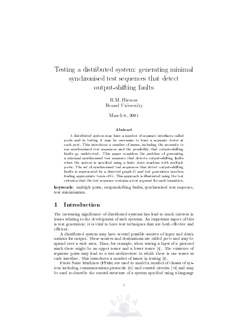
A plane tree τ with p edges (or p + 1 vertices)
Göteborg
7 / 40
Important special cases
Geometric distribution µ(k) = 2−k −1 Then, if |τ | = number of edges of τ , P(θ = τ ) = 2−2|τ |−1. Consequence: The conditional distribution of θ given |θ| = p is uniform over {plane trees with p edges}. e−1 k! The conditional distribution of θ given |θ| = p is uniform over {Cayley trees on p + 1 vertices}. (Needs to view a plane tree as a Cayley tree by “forgetting” the order and randomly assigning labels 1, 2, . . . to vertices) µ(k) =
Jean-François Le Gall (Université Paris-Sud)
Random treesare we aiming at?
output-shifting
such as SDL, Estelle or Statecharts 18, 15, 12, 11]. While speci cations in these languages are usually extended nite state machines ( nite state machines with data) rather than FSMs, these may be converted to FSMs by either applying some abstraction or expanding out the data (after making the ranges nite). This has lead to interest in the automatic generation of tests from FSMs (see, for example, 1, 24, 9, 10, 22]). Traditionally, the interest in FSM based testing has largely been limited to protocol conformance testing and the testing of embedded control system. However, the use of Statecharts within the UML has recently widened the interest in this topic. When testing a system with multiple ports, there is one (local) tester at each port. Suppose testing involves the input of x at port p and then x0 at port p0 (p 6= p0 ). In order for the tester at p0 to know when to input x0 it must know when x has been input. If the tester at p0 does know when x has been input, because it has received output from the transition triggered by x, these two tests are synchronised. Sometimes there is no synchronised test that satis es the test criterion 19]. When this is the case, it may be possible to allow the testers to communicate: local testers may send synchronisation messages to one another. It is then possible to produce a synchronised test sequence. Naturally, when considering test minimisation, the cost of the synchronisation messages should be included. Thus, approaches that produce test sequences and then add synchronising messages may be suboptimal. Normally the testing problem is further complicated by the absence of a global clock 16]. In the presence of multiple ports, this reduces the ability of the test system to determine the global order of the input and output. It will be assumed that there is no global clock. When there are multiple ports, the lack of a global clock may make it di cult to determine which input triggered a particular output value. This makes it di cult to detect output being shifted between adjacent transitions in a test. Faults that shift output between adjacent tests are called output-shifting faults. Suppose, for example, that the tester at port p1 is to input x, this is expected to lead to a2 and a3 being output at ports p2 and p3 respectively, the tester at port p2 is then to input x0 and this is expected to lead to output of a4 at port p4 . This test sequence is synchronised as the tester at port p2 inputs x0 after it has received output a2 . However, it is possible that the input values trigger the wrong output but no fault is detected. For example, if the input of x leads to the output of a2 and a4 at p2 and p4 respectively and the input of x0 leads to the output of a3 at p3, the correct behaviour is seen at each port. The sequencing of these two transitions has allowed the faults to mask one another. While these faults are not detected in testing they might lead to problems when the system is used. Other authors have considered related problems. 16] introduce the term output-shifting fault and note that a synchronised test sequence need not detect output-shifting faults. 3] show how a minimalset of messages may be added to a given test sequence to produce a synchronised test sequence that detects outputshifting faults. However, where the initial test sequence has been produced to 2
Ladder图和M

Ladder图和M bius Ladder图的彩虹点连通数(英文)刘慧敏;毛亚平【期刊名称】《数学季刊:英文版》【年(卷),期】2016(31)4【摘要】A vertex-colored graph G is said to be rainbow vertex-connected if every two vertices of G are connected by a path whose internal vertices have distinct colors, such a path is called a rainbow path. The rainbow vertex-connection number of a connected graph G, denoted by rvc(G), is the smallest number of colors that are needed in order to make G rainbow vertex-connected. If for every pair u, v of distinct vertices, G contains a rainbow u-v geodesic, then G is strong rainbow vertex-connected. The minimum number k for which there exists a k-vertex-coloring of G that results in a strongly rainbow vertex-connected graph is called the strong rainbow vertex-connection number of G, denoted by srvc(G). Observe that rvc(G) ≤ srvc(G) for any nontrivial connected graph G. In this paper, for a Ladder L_n,we determine the exact value of srvc(L_n) for n even. For n odd, upper and lower bounds of srvc(L_n) are obtained. We also give upper and lower bounds of the(strong) rainbow vertex-connection number ofM bius Ladder.【总页数】7页(P399-405)【关键词】vertex-coloring;rainbow vertex-connection;(strong) rainbow vertex-connection number;Ladder;M bius Ladder【作者】刘慧敏;毛亚平【作者单位】Department of Mathematics,Qinghai Normal University【正文语种】中文【中图分类】O【相关文献】1.三类特殊图的(强)彩虹连通数 [J], 赵燕;柴航2.一些特殊图的Mycielskian图的彩虹顶点连通数 [J], 张璐;边红3.小直径二连通外平面图的彩虹连通数 [J], 邓兴超;宋贺;苏贵福;田润丽4.一些特殊定向图及其Mycielskian图的彩虹连通数 [J], 刘敏;边红;于海征;赵菲菲5.关于有限群幂图的强彩虹连通数 [J], MA Xuan-long;SU Hua-dong因版权原因,仅展示原文概要,查看原文内容请购买。
automesh子面板详细解释

HyperMesh and BatchMesherAutomesh PanelHyperWorks Desktop Applications > HyperMesh > User's Guide > HyperMesh Panels > HyperMesh Panels Listed Alphabetically:Automesh PanelLocation: The Automesh panel can be accessed from the menu bar by clicking Mesh > Create > 2D Automesh, or by pressing the F12 functionkey.The Automesh panel is used to generate a mesh of plate elements using surface geometry or existing shell elements to define the mesh area.Panel UsageThe options in the panel can be set in any order that you feel comfortable using. Moving from subpanel to subpanel will not cause you to lose work. When finished making all your selections, start the meshing process using the mesh button on the right side of the panel.•Set the panel mode by selecting the appropriate subpanel•Select the meshing method by setting the entity selector to surfs or elems•Make the required element criteria settings•Set any algorithm options•Select the area to be meshed using the entity selector and any extendedselection methods desired.Note:The unmeshed and failed selection buttons on the right side of the panel can be used to make pre-defined surface selections if desired.Subpanels and InputsThe Automesh panel contains the following subpanels:Size and BiasSize and bias meshing is a very flexible and powerful meshing method. A minimum of inputs are required for the element criteria settings. The algorithm options can set preferences on how to handle certain situations when encountered in the geometry. When using existing finite elements as the basis for mesh generation, feature recognition settings allow the mesher to break up the areas defined by the selected elements into logical groupings with mesh controls set for each group boundary.This meshing mode works interactively or automatically. In interactive mode, a great deal of manual control is presented via the Secondary Automesh panel during the mesh generation stage. Interactive meshing allows you to control mesh size and element type, and to set different mesh generation algorithms and test element quality on a surface-by-surface basis. The resulting modified mesh can be updated at any time, giving immediate feedback as to the effectiveness of the change. When meshing in the automatic mode, the mesh will be generated using only the settings, criteria and options set in the Automesh panel.Size and biasing produces a mesh with consistent element size. If meshed interactively, the number of elements (element density) node spacing (biasing), element type and mesh style can be modified for each surface face and edge.Panel Inputs•Quads attempts to use quads only--however, at least one triaelement must be created if the sum of the element densities around the perimeter of the face or surface is odd.The sum of element densities on the perimeter of thelower surface is odd, resulting in a tria as indicated.Adjusting the element densities while meshing interactively can usually elimate all tria elements.Adjusting the bottom edge density from 11 to 10 makesthe sum even and allows all-quads to be generated.•Quads only uses a subdividing routine that tends to generate more orthogonal quad elements.Tria elements may still be introduced depending on thedensity settings as with the quads type.•Tria elements uses all-trias to mesh.•R-trias are right-angle triangular elements.If you select Advanced, choose any of the other types individually for mapped elements (elements on surfaces that can be mapped to simple geometric shapes) and free elements (those that cannot easily map to simple shapes).tAmap as circle - free map as circle - mapped map as rectangle - free map as rectangle - mapped map as pentagon - free map as pentagon - mappedAny time two adjacent elements’ normals would e xceed this angle HyperMesh creates a new set of nodes between them to maintain clean feature lines. Using a higher value results in elements spanning the feature line:With an appropriate value, the features lines are preserved.If feature angle = is too high, the feature lines are blurred.Produce a more orthogonal quad-dominant mesh. Only applies to mixed element type.Here, there is no flow alignmentFlow alignment is used, producing straighter rows of elementsMesh without link opposite edges Mesh with link oppositeedgesMesh with link oppositeedgesQI OptimizeQuality Index meshing is an iterative automatic mesh generation method driven by element quality criteria. During the mesh generation process, the quality index of the mesh is determined by evaluating each element against a set of element quality tests. If all required element quality criteria are passed, then that element has a perfect quality index of zero. As the element quality deteriorates, the quality index value increases; so a lower quality index score indicates an element more closely meets the ideal quality requirements.The compound quality index sum of the quality index values for each of the elements that are included in the current meshing area. The quality index value itself has no direct physical meaning; it is a way to compare one generated mesh pattern against another pattern generated for that same area. The quality index based mesh optimization routine attempts modify the mesh pattern and apply node smoothing routines to obtain a lower overall quality index value.For more on element quality index, see the Quality Index panel.Panel InputsSelect quads, trias, mixed, or Quads only to specify the type of element to use in building meshes.•Mixed uses quads primarily, but inserts trias whenmaking density transitions, resulting in improved mesh quality.•Quads attempts to use quads only--however, at leastone tria element must be created if the sum of theelement densities around the perimeter of the face orsurface is odd.Adjusting the element densities while meshinginteractively can usually eliminate all tria elements.•Quads only uses a subdividing routine that tends to generate more orthogonal quad elements.Tria elements may still be introduced depending onthe density settings as with the quads type.•Tria elements uses all-trias to mesh.Specify a maximum angle across which elements can be maintained.Any time two adjacent elements’ normals would exceed this angle HyperMesh creates a new set of nodes between them to maintain clean feature lines. Using a higher value results in elements spanning the feature line:With an appropriate value, the features lines are preserved.If feature angle = is too high, the feature lines are blurred.Produce a more orthogonal quad-dominant mesh. Only applies to mixed element type.Here, there is no flow alignmentFlow alignment is used, producing straighter rows of elements•flow: align produces a more orthogonal quad dominated mesh•flow: size appears only when align is active, andEdge DeviationUse the Edge Deviation subpanel to set specific meshing parameters to limit how far the mesh elements can deviate from the actual edges of the surfaces meshed, or when in the case of re-meshing elements, deviation from inferred edges based on features.Controls for the minimum and maximum allowable element size, edge deviation and maximum angle are introduced with this method. Edge deviation normally occurs on curved edges, because individual elements have straight edges and therefore can only approximate a curve.When meshing curved surfaces as shown here, the planar elements (tan color) can deviate from the curved greygeometry.Edge deviation applies to both surface geometry and when re-meshing elements. Automeshing on the edge deviation subpanel automatically selects the best element size to approximate a curve, within the limits that you specify. The max deviation and max angle settings are the primary controls for this effect.This method can produce a mesh in which the element size varies, even within the same surface. Areas of high curvature will tend to have smaller elements than areas of low or no curvature. The element size boundaries allow you to control this effect.Edge deviation control when meshing creates smaller elements and spaces nodes closer together to limit how much the elements can deviate from the surface edges.Panel Inputs•Quads attempts to use quads only--however, at least one triaelement must be created if the sum of the element densities around the perimeter of the face or surface is odd.Adjusting the element densities while meshing interactively can usually eliminate all tria elements.•Quads only uses a subdividing routine that tends to generate more orthogonal quad elements.Tria elements may still be introduced depending on thedensity settings as with the quads type.•Tria elements uses all-trias to mesh.•R-trias are right-angle triangular elements.If you select Advanced, choose any of the other types individually for mapped elements (elements on surfaces that can be mapped to simple geometric shapes) and free elements (those that cannot easily map to simple shapes).map as circle - free map as circle - mappedmap as pentagon - free map as pentagon - mappedSpecify a maximum angle across which elements can be maintained.Any time two adjacent elements’ normals would exceed this angle HyperMesh creates a new set of nodes between them to maintain clean feature lines. Using a higher value results in elements spanning the feature line:With an appropriate value, the features lines are preserved.If feature angle = is too high, the feature lines are blurred.Produce a more orthogonal quad-dominant mesh. Only applies to mixed element type.Here, there is no flow alignmentFlow alignment is used, producing straighter rows of elements•flow: align produces a more orthogonal quad dominated mesh•flow: size appears only when align is active, and enforces theglobal mesh element size with minimal min/max element size variation.Mesh without link opposite edges with AR < selected.Mesh with link oppositeedgeswith AR < set to auto.Mesh with link oppositeedgeswith AR < set to 8.0.Surface Deviation (surface meshing only)This subpanel is only accessible when meshing surfaces. Use the Surface Deviation subpanel to mesh within limits of element deviation from a surface.Similarly to the edge deviation subpanel, meshing behavior on this subpanel is driven by distances between flat elements and model geometry. When flat elements are used to approximate a curved surface, there is always a discrepancy between each element and the actual curve of the surface, because the element uses a straight line between two nodes:A gap is visible between the curved edge of the surface and the element edges.The surface deviation automesh method chooses the mesh density based on the severity of this deviation. Where the threshold deviation would be exceeded, smaller elements are used to reduce the deviation:With surface deviation meshing, smaller elements are used to accuratelyrepresent curved surfaces. Larger elements are used where the geometry showsless curvature.The surface deviation meshing works only in an automatic mode; interactive meshing with the secondary automesh panel is not possible. However, the refine function can be used to set a specific desired mesh size for a point, line or surface face. This option accesses another temporary subpanel that is slaved to the surface deviation subpanel, and allows you to select fixed points, lines, or surfaces to define an area in which you desire a more refined mesh. You can specify a different element size for these areas, which displays as a color-coded numeric value: yellow for points, green for lines, or red for surfaces. An option to show all or show active toggles the view of these numeric values; show active displays only the refinement value for the most recently selected point, line or surface, while show all shows all values for all selected entities.After specifying refinement options, clicking mesh causes the meshing engine to create a smoothly-scaled mesh from your base element size to the size specified inthe refine options.Here, the mesh is not refined, but the colored numbers indicate refinement targets: point (yellow), line (green), and surface (red)Here, refinement is applied. You can see that the mesh is finer near the point (yellow), along the line/edge (green), and on the surface (red).Panel InputsDetermines how rapidly elements can increase in size as they are created further and further away from features.Elements further from the features grow larger with each row.maintain clean feature lines. Using a higher value results in elements spanning the feature line:With an appropriate value, the features lines are preserved.If feature angle = is too high, the feature lines are blurred.Select quads, trias, mixed, R-trias, Quads only, or advanced to specify the type of element to use in building meshes.•Mixed uses quads primarily, but inserts trias when making density transitions, resulting in improved mesh quality.•Quads attempts to use quads only--however, at least onetria element must be created if the sum of the element densities around the perimeter of the face or surface is odd.Adjusting the element densities while meshinginteractively can usually eliminate all tria elements.•Quads only uses a subdividing routine that tends to generate more orthogonal quad elements.Tria elements may still be introduced depending on the density settings as with the quads type.•Tria elements uses all-trias to mesh.•R-trias are right-angle triangular elements.If you select Advanced, choose any of the other types individually for mapped elements (elements on surfaces that can be mapped to simple geometric shapes) and free elements (those that cannot easily map to simple shapes).map as circle - free map as circle - mappedmap as pentagon - free map as pentagon - mappedUse the Rigid Body Mesh subpanel to create a quick mesh to represent the topology of a rigid object. Only the automatic meshing mode is available.Rigid bodies are surfaces that are expected to be treated as undeformable in the solution. One example of a rigid body is in metal-forming. When modeling the results of a die pressing down on a metal sheet, it’s important to model the shape of the die because that determines the shape of the metal sheet after being pressed. However, during a forming analysis the stresses and deformations of thedie itself are not of interest, only those of the formed metal sheet. Otherapplications for rigid bodies include the impactors used in vehicle crash simulation.A mesh that accurately represents the rigid geometry is important for such simulations to allow the solver collision detection routines to work effectively and accurately. Since stress and deformation of the rigid body are not calculated by the solver, the rigid body mesh focuses on accurately modeling the shape of the body rather than on producing a high-quality mesh. To this end, it uses the same faceting and shading routines that are used for drawing the model graphics. The resulting mesh may have high aspect ratio or extremely tapered elements that would not be suitable for solution, but can accurately represent the geometry.The images below illustrate the differences between surface deviation meshing and rigid body meshing. Both meshes were generated using the same parameters in terms of min/max element size, maximum deviation and feature angle, and mesh type.When creating a surface deviation based mesh on this cone, many small elements are required to capture the geometry, even so, the elements exhibit a lot of warpage and those at the tip are distorted and do not accurately represent the geometry.With the rigid body mesh, the shape of the object can be accurately modeled using fewer larger elements since the element shape is not a concern.Panel InputsSpecify a maximum allowable break angle between adjacent elements. The element size is adjusted such that the angle between the normals of adjacent elements does not exceed this value.In these examples, the minimum and maximum element sizes are 3 and50 respectively. In this first image, the mesh is constrained by the max deviation value set to 0.5. The element size is set such that the maximum distance between the element and the spherical surface does not exceed this setting.In this second example, the deviation setting is relaxed to 3.0, and the mesh is bound by the maximum feature angle setting of 45 degrees.•Tria elements uses all-trias to mesh.See Also:HM-3100: AutoMeshingHM-3120: 2-D Mesh in Curved Surfaces HM-3130: QI Mesh CreationQuality Index panelAn Alphabetical List of HyperMesh Panels An Alphabetical List of HyperForm Panels。
《群论》部分习题答案
《群论》部分习题解答版权所有人:Wu TS,2006年4月第一章.预备知识(Chapter1.Preliminary) 4.(Page28)Let S be the set of all n×n symmetric real matrices and in S we define a binary relation∼in the followingA∼B if and only if there exists an invertible matrix C such that B=C AC,where C is the transpose matrix of C.Prove that∼defines an equivalent relation in pute|S/∼|.解答:(1)直接验证∼是S的一个等价关系。
(2)根据线性代数理论,对于任意实对称矩阵A,存在可逆矩阵Q 使得Q AQ是对角矩阵diag{1,1,···,−1,···,−1,0,···,0},简记为Q AQ=E r000−E s0000=Dr,s,其中r+s=r(A).根据惯性定理,其中的r也是由A唯一确定的。
因此,两个n阶实对称矩阵A与B合同的充分必要条件是r(A)=r(B)且正惯性指数相同。
所以我们得到S/∼={D r,s|0≤r,s and r+s≤n},其中,D r,s={P D r,s P|P∈GL n(R)}.下面计算|S/∼|.(1)满足r=0的D r,s共有n+1个,它们分别是D0,0,D0,1,D0,2,···,D0,n.(2)满足r=1的D r,s共有n个,它们分别是D1,0,D1,1,D1,2,···,D1,n−1.···(n+1)满足r=n的D r,s共有1个,即为D n,0.因此,|S/∼|=n+1j=1j=(n+1)(n+2)2.1第二章.群论(Chapter2.Group Theory)1.(Page49)Prove that both G1={(a ij)n×n|a ij∈Z,det(A)=1}and G2= {(a ij)n×n|a ij∈Q,det(A)=1}are groups under the matrix multiplication.证明:只证明G1是子群。
Memory bandwidth bottleneck and its amelioration by a compiler
The Memory Bandwidth Bottleneck and its Amelioration by a CompilerChen Ding Ken KennedyRice University,Houston,Texas,USA{cding,ken}@AbstractAs the speed gap between CPU and memory widens, memory hierarchy has become the primary factor limiting program performance.Until now,the principal focus of hardware and software innovations has been overcoming latency.However,the advent of latency tolerance tech-niques such as non-blocking cache and software prefetch-ing begins the process of trading bandwidth for latency by overlapping and pipelining memory transfers.Since actual latency is the inverse of the consumed bandwidth,mem-ory latency cannot be fully tolerated without infinite band-width.This perspective has led us to two questions.Do current machines provide sufficient data bandwidth?If not, can a program be restructured to consume less bandwidth? This paper answers these questions in two parts.Thefirst part defines a new bandwidth-based performance model and demonstrates the serious performance bottleneck due to the lack of memory bandwidth.The second part describes a new set of compiler optimizations for reducing bandwidth consumption of programs.1IntroductionAs modern single-chip processors improve the rate at which they execute instructions,it has become increasingly the case that the performance of applications depends on the performance of the machine memory hierarchy.For some years,there has been an intense focus in the compiler and architecture community on ameliorating the impact of mem-ory latency on performance.This work has led to extremely effective techniques for reducing and tolerating memory la-tency,primarily through cache reuse and data prefetching.As exposed memory latency is reduced,memory band-width consumption is increased.For example,when CPU simultaneously fetches two data items from memory,the actual latency per access is halved,but the memory band-width consumption is doubled.Since actual latency is the inverse of the consumed bandwidth,memory latency can-not be fully tolerated without infinite bandwidth.Indeed on any real machine,program performance is bounded by the limited rate at which data operands are delivered into CPU, regardless of the speed of processors or the physical latency of data access.Because of the past focus on memory latency,the band-width constraint had not been carefully studied nor had the strategy of bandwidth-oriented optimization.The purpose of this paper is to address these two important issues.The first part of the paper introduces a bandwidth-based perfor-mance model and presents a performance study based on this model.By measuring and comparing the demand and supply of data bandwidth on all levels of memory hierarchy, the study reveals the serious performance bottleneck due to the lack of memory bandwidth.The second part of the paper presents new compiler op-timizations for reducing bandwidth consumption of a pro-gram.Unlike memory latency which is a local attribute of individual memory references,bandwidth consumption of a program is a global property of all memory access. Therefore,a compiler needs to transform the whole pro-gram,not just a single loop nest.In addition,since memory writebacks equally consumes bandwidth as memory reads, a compiler needs to optimize data stores,not just data loads. For these purposes,this paper introduces three new tech-niques.Thefirst is bandwidth-minimal loop fusion,which studies how to organize global computation so that the to-tal amount of memory transfer is minimized.The second is storage reduction,which reduces the data footprint of com-putation.The last one is store elimination,which removes writebacks to program data.These three techniques form a compiler strategy that can significantly alleviate the prob-lem of memory bandwidth bottleneck.The rest of the paper is organized as follows.Section2 defines the bandwidth-based performance model and mea-sures the memory bandwidth bottleneck.Section3de-scribes three new compiler transformations for bandwidth reduction.Section4discusses related work and Section5 summarizes.2Memory bandwidth bottleneckThis sectionfirst shows an example where memory la-tency is clearly not the primary constraint on performance. The most serious constraint is memory bandwidth,as stud-ied in the rest of the section.2.1A simple exampleThe example program has two loops performing stride-one access to a large data array.The only difference is that thefirst one also writes the array back to memory.Since both loops perform the same reads,they should have the same latency and the same performance if latency is the de-termining factor.Both loops also have the same number of floating-point operations.double precision A[2000000]for i=1to NA[i]=A[i]+0.4end forfor i=1to Nsum=sum+A[i]end forSurprisingly,thefirst loop takes0.104second on a R10K processor of SGI Origin2000,which is almost twice the execution time of the second loop,0.054second.On HP/Convex Exemplar,thefirst loop takes0.055second and the second0.036.The reason,as shown next,is that the per-formance is determined by memory bandwidth,not memory latency.Thefirst loop takes twice as long because it writes the array to memory and consequently consumes twice as much memory bandwidth.2.2Program and machine balanceTo understand the supply and demand of memory band-width as well as other computer resources,it is necessary to go back to the basis of computing systems,which is the bal-ance between computation and data transfer.This section first formulates a performance model based on the concept of balance and then uses the model to examine the perfor-mance bottleneck on current machines.Both a program and a machine have balance.Program balance is the amount of data transfer(including both data reads and writes)that the program needs for each computa-tion operation;machine balance is the amount of data trans-fer that the machine provides for each machine operation. Specifically,for a scientific program,the program balance is the average number of bytes that must be transferred per floating-point operation(flop)in the program;the machinePrograms Program/machine BalanceL1-Reg Mem-L26.4 5.2dmxpy8.324.0 5.9mm(-O3)0.978.3 2.7NAS/SP 6.415.07.840.8Figure1.Program and machine balance balance is the number of bytes the machine can transfer per flop in its peakflop rate.On machines with multiple lev-els of cache memory,the balance includes the data transfer between all adjacent levels.The table in Figure1compares program and machine balance.The upper half of the table lists the balance of six representative scientific applications1,including four kernels—convolution,dmxpy,matrix multiply,FFT—and two application benchmarks—SP from the NAS benchmark suite and Sweep3D from DOE.For example,thefirst row shows that for eachflop,convolution requires transferring 6.4bytes between the level-one cache(L1)and registers, 5.1bytes between L1and the level-two cache(L2),and 5.2bytes between L2and memory.The last row gives the balance of a R10K processor on SGI Origin20002,which shows that for eachflop at its peak performance,the ma-chine can transfer4bytes between registers and cache,4 bytes between L1and L2,but merely0.8bytes between cache and memory.As the last column of the table shows,with the exception of mm(-O3),all applications demand a substantially higher rate of memory transfer than that provided by Origin2000. The demands are between2.7to8.4bytes perflop,while the supply is only0.8byte perflop.The striking mismatch clearly confirms the fact that memory bandwidth is a serious performance bottleneck.In fact,memory bandwidth is the least sufficient resource because its mismatch is much larger than that of register and cache bandwidth,shown by the sec-ond and the third column in Figure1.The next section will take a closer look at this memory bandwidth bottleneck.The reason matrix multiply mm(-O3)requires very little memory transfer is that at the highest optimization level of -O3,the compiler performs advanced computation block-Applications Ratios of demand over supplyL1-Reg Mem-L21.6 6.5dmxpy 2.16.07.4FFT0.82.7 6.1Sweep3D 2.33We suspect that3w6r kernel causes excessive cache conflicts becauseit accesses6large arrays on a direct-mapped cache.Cache conflicts re-sult in a much higher amount of data transfer,which we cannot measurebecause of the absence of hardware counters on Exemplarthat5out of its7major computation subroutines utilized 84%or higher of the memory bandwidth of Origin2000. The high bandwidth utilization shows that memory band-width is the major performance bottleneck for SP,and the bandwidth saturation we see on those kernels is indeed hap-pening on full applications as well.We cannot measure the bandwidth utilization of SP on Exemplar because of the ab-sence of hardware counters.The kernels represent difference patterns of stride-one memory access.NAS/SP is a real application with regu-lar data access patterns and a large amount of computation. Since they together resembles many programs with regular computations,their effective bandwidth suggest that regular applications saturate memory bandwidth most of the times. In these cases,memory bandwidth is a more limiting factor to performance than is memory latency.In conclusion,the empirical study has shown that for most applications,machine memory bandwidth is between one third and one tenth of that needed.As a result,over80% of CPU power is left un-utilized by large applications,indi-cating a significant performance potential that may be real-ized if the applications can better utilize the limited memory bandwidth.The next section introduces new compiler tech-niques that are aimed at exactly this goal,that is,reducing the memory bandwidth demand of applications.3Bandwidth reduction by a compiler This section presents a compiler strategy for reducing the bandwidth consumption of a program.Thefirst tech-nique is a new formulation of loop fusion,which minimizes the overall data transfer among fused loops.One effect of global loop fusion is the localized live range of arrays.The next two techniques exploit this opportunity and further re-duce the bandwidth consumption after loop fusion,includ-ing the unique opportunity of eliminating memory write-backs.3.1Bandwidth-minimal loop fusionThis sectionfirst formulates the problem of loop fu-sion for minimal memory transfer,then gives a polynomial solution to a restricted form of this problem,andfinally proves that the complexity of the unrestricted form is NP-complete.In the process,it also points out why the previous fusion model given by Gao et al.[5]and by Kennedy and McKinley[7]does not minimize bandwidth consumption.3.1.1FormulationGiven a sequence of loops accessing a set of data arrays, Gao et al.[5]and by Kennedy and McKinley[7]modeled both the computation and the data in a fusion graph.A fu-sion graph consists of nodes—each loop is a node—and two types of edges—directed edges for modeling data de-pendences and undirected edges for fusion-preventing con-straints.Our formulation uses the same definition of a fu-sion graph.However,the objective of fusion is a different one,as stated below.Problem3.1Bandwidth-minimal fusion problem: Given a fusion graph,how can we divide the nodes into a sequence of partitions such that•(Correctness)each node appears in one and only onepartition;the nodes in each partition have no fusionpreventing constraint among them;and dependenceedgesflow only from an earlier partition to a laterpartition in the sequence,•(Optimality)the sum of the number of distinct arraysin all partitions is minimal.The correctness constraint ensures that loop fusion obeys data dependences and fusion-preventing constraints.As-suming arrays are large enough to prohibit cache reuse among disjoint loops,the second requirement ensures opti-mality because for each loop,the number of distinct arrays is the number of arrays the loop reads from memory during execution.Therefore,the minimal number of arrays in all partitions means the minimal memory transfer and minimal bandwidth consumption for the whole program.For example,Figure4shows the fusion graph of six loops.Assuming that loop5and loop6cannot be fused, but either of them can be freely fused with any other four loops.Loop6depends on loop5.Without fusion,the total number of arrays accessed in the six loops is20.The op-timal fusion leaves loop5alone and fuses all other loops. The number of distinct arrays is1in thefirst partition and 6in the second,thus the total memory transfer is reduced from20arrays to7.The optimality of bandwidth-minimal fusion is different from previous work on loop fusion of Gao et al.[5]and Kennedy and McKinley[7].They modeled data reuse as weighted edges between graph nodes.For example,the edge weight between loop1and2would be4because they share four arrays.Their goal is to partition the nodes so that the total weight of cross-partition edges is minimal.We call this formulation edge-weighted fusion.The sum of edge weights does not correctly model the aggregation of data reuse.For example,in Figure4,loop 1to3each has a single-weight edge to loop5.But the aggregated reuse between thefirst three loops and loop5 should not be3;on the contrary,the amount of data sharing is1because they share access to only one array,A.Data Arrays: A, B, C, D, E, F Loop 6Scalar Data: sumFigure 4.Example loop fusionTo show that edge-weighted fusion does not minimize bandwidth consumption,it suffices to give a counter ex-ample,which is the real purpose of Figure 4.The optimal edge-weighted fusion is to fuse the first five loops and leave loop 6alone.The total weight of cross-partition edges is 2,which lies between loop 4and 6.However,this fusion has to load 8arrays (6in the first partition and 2in the second),while the previous bandwidth-minimal fusion needs only 7.Reversely,the total weight of inter-partition edges in the bandwidth-minimal fusion is 3,clearly not optimal based on the edge-weighted formulation.Therefore,the previous formulation by Gao et al.and Kennedy and McKinley does not minimize overall memory transfer.To understand the effect of data sharing and the complex-ity of bandwidth-minimal fusion,the remaining part of this section studies a model based on a different type of graphs,hyper-graphs.3.1.2Solution Based On Hyper-graphsThe traditional definition of an edge is inadequate for mod-eling data sharing because the same data can be shared by more than two loops.Instead,the following formulation uses hyper-graphs because a hyper-edge can connect any number of nodes in a graph.A graph with hyper-edges is called a hyper-graph .The optimality requirement of loop fusion can now be restated as follows.Problem 3.2Bandwidth-minimal fusion problem (II):Given a fusion graph as constructed by Problem 3.1,add a hyper-edge for each array in the program,which connects all loops that access the array.How can we divide all nodes into a sequence of partitions such that•(Correctness)criteria are the same as Problem 3.1,but•(Optimality)for each hyper-edge,let the length be the number of partitions the edge connects to after parti-tioning,then the goal is to minimize the total length of all hyper-edges.The next part first solves the problem of optimal two-partitioning on hyper-graphs and then proves the NP-completeness of multi-partitioning.Two-partitioning is a special class of the fusion problem where the fusion graph has only one fusion-preventing edge and no data dependence edge among non-terminal nodes.The result of fusion will produce two partitions where any non-terminal node can appear in any partition.The example in Figure 4is a two-partitioning problem.Two-partitioning can be solved as a connectivity prob-lem between two nodes.Two nodes are connected if there is a path between them.A path between two nodes is a sequence of hyper-edges where the first edge connects one node,the last edge connects the other node,and consecutive ones connect intersecting groups of nodes.Given a hyper-graph with two end nodes,a cut is a set of hyper-edges such that taking out these edges would dis-connect the end nodes.In a two-partitioning problem,any cut is a legal partitioning.The size of the cut determines the total amount of data loading,which is the total size of the data plus the size of the cut (which is the amount of data reloading).Therefore,to obtain the optimal fusion is to find a minimal cut.The algorithm given is Figure 5finds a minimal cut for a hyper-graph.At the first step,the algorithm transforms the hyper-graph into a normal graph by converting each hyper-edge into a node,and connecting two nodes in the new graph when the respective hyper-edges overlap.The conversion also constructs two new end nodes for the trans-formed graph.The problem now becomes one of finding minimal vertex cut on a normal graph.The second step applies standard algorithm for minimal vertex cut,which converts the graph into a directed graph,splits each node into two and connects them with a directed edge,and fi-nally finds the edge cut set by the standard Ford-Fulkerson method.The last step transforms the vertex-cut to the hyper-edge cut in the fusion graph and constructs the two partitions.Although algorithm in Figure 5can find minimal cut for hyper-edges with non-negative weights,we are only con-cerned with fusion graphs where edges have unit-weight.In this case,the first step of the minimal-cut algorithm in Fig-ure 5takes O (E +V );the second step takes O (V ′(E ′+V ′))if breadth-first search is used to find augmenting paths;fi-nally,the last step takes O (E +V ).Since V ′=E in the second step,the overall cost is O (E (E ′+E )+V ),where E is the number of arrays,V is the number of loops and E ′is the number of the pair of arrays that are accessed by the same loop.In the worst case,E ′=E 2,and the algo-Input A hyper-graph G=(V,E).Two nodes s and t∈V.Output A set of edges C(a minimal cut between s and t).Two partitions V1and V2,where s∈V1,t∈V2,V1=V−V2,and e connects V1and V2iff e∈C. Algorithm/*Initialization*/let C,V1and V2be empty sets/*Step1:convert G to a normal graph G’*/ construct a normal graph G’=(V’,E’)let array map[]maps from V’to Efor each e in E,add a node v to V’let map[v]=eadd edge(v1,v2)in G’iff map[v1]and map[v2]overlap in G /*add two end nodes to G’*/add two new nodes s’and t’to V’for each node v in V’add edge(s’,v)if map[v]contains s in Gadd edge(t’,v)if map[v]contains t in G/*Step2:minimal vertex cut in G’*/convert G’into a directed graphsplit each node in V’andadd in a directed edge in between use For-Fulkerson method to find theminimal edge cut between s’and t’convert the minimal edge cut into thevertex cut in G’/*Step3:construct the cut set in G*/let C be the vertex cut set found in step2 delete all edges of G corresponding to nodes in Clet V1be the set of nodes connected to s in G;let V2be V-V1return C,V1and V2Figure5.Minimal-cut for hyper-graphs rithm takes O(E3+V).What is surprising is that although the time is cubic to the number of arrays,it is linear to the number of loops in a program.By far the solution method has assumed the absence of dependence edges.The dependence relation can be en-forced by adding hyper-edges to the fusion graph.Given a fusion graph with N edges and two end nodes s and t,as-sume the dependence relations form an acyclic graph.Then if node a depends on b,we can add three sets of N edges connecting s and a,a and b,and b and t.Minimal-cut will stillfind the minimal cut although each dependence adds a weight of N to the total weight of minimal cut.Any de-pendence violation would add an extra N to the weight of a cut,which makes it impossible to be minimal.In other words,any minimal cut will not place a before b,and the de-pendence is observed.However,adding such edges would increase the time complexity because the number of hyper-edges will be in the same order as the number of dependence edges.3.1.3The Complexity of General Loop Fusion Although the two-partitioning problem can be solved in polynomial time,the multi-partitioning form of bandwidth-minimal fusion is NP-complete.To prove,observe that the fusion problem is in NP be-cause loops or nodes of a fusion graph can be partitioned in a non-deterministic way,and the legality and optimality can be checked in polynomial time.The fusion problem is also NP-hard.To prove this,we reduce k-way cut problem to the fusion problem.Given a graph G=(V,E)and k nodes to be designated as termi-nals,k-way cut is tofind a set of edges of minimal total weight such that removing the edges renders all k termi-nals disconnected from each other.To convert a k-way cut problem to a fusion problem,we construct a hyper-graph G′=(V′,E′)where V′=V.We add in a fusion-preventing edge between each pair of terminals,and for each edge in E,we add a new hyper-edge connecting the two end nodes of the edge.It is easy to see that a minimal k-way cut in G is an optimal fusion in G′and vice versa. Since k-way cut is NP-complete,bandwidth-minimal fu-sion is NP-hard when the number of partitions is greater than two.Therefore,it is NP-complete.Aggressive fusion enables other optimizations.For ex-ample,the use of an array can become enclosed within one or a few loops.The localized use allows aggressive storage transformations that are not possible otherwise.The rest of this section describes two such storage optimizations:stor-age reduction,which replaces a large array with a small sec-tion or a scalar;and store elimination,which avoids writing back new values to an array.Both save a significant amount more memory bandwidth than loop fusion.3.2Storage ReductionAfter loop fusion,if the live range of an array is short-ened to stay within a single loop nest,the array can be re-placed by a smaller data section or even a scalar.In par-ticular,two opportunities exist for storage reduction.The first case is where the live range of a data element(all uses of the data element)is short,for example,within one loop iteration.The second case is where the live range spans the whole loop,but only a small section of data elements have such a live range.Thefirst case can be optimized by array shrinking,where a small temporary buffer is used to carry live ranges.The second case can be optimized by array peeling,where only a reduced section of an array is saved in a dedicated storage.Figure6illustrates both transforma-tions.The example program in Figure6(a)uses two large ar-rays a[N,N]and b[N,N].Loop fusion transforms the pro-gram into Figure6(b).Not only does the fused loop con-tain all accesses to both arrays,the definitions and uses of many array elements are very close in computation.The live range of a b-array element is within one iteration of the in-ner loop.Therefore,the whole b array can be replaced by a scalar b1.The live range of an a-array element is longer,but it is still within every two consecutive j iterations.There-fore,array a[N,N]can be reduced into a smaller buffer a3[N],which carries values from one j iteration to the next.A section of a[N,N]array has a live range spanning the whole loop because a[1...N,1]is defined at the beginning and used at the end.These elements can be peeled off into a smaller array a1[N]and saved throughout the loop.After array shrinking and peeling,the original two arrays of size N2have been replaced by two arrays of size N plus two scalars,achieving a dramatic reduction in storage space.Storage reduction directly reduces the bandwidth con-sumption between all levels of memory hierarchy.First,the optimized program occupies a smaller amount of memory, resulting in less memory-CPU transfer.Second,it has a smaller footprint in cache,increasing the chance of cache reuse.When an array can be reduced to a scalar,all its uses can be completed in a register,eliminating cache-register transfers as well.3.3Store EliminationWhile storage reduction optimizes only localized ar-rays,the second transformation,store elimination,improves bandwidth utilization of arrays whose live range spans mul-tiple loop nests.The transformationfirst locates the loop containing the last segment of the live range and thenfin-ishes all uses of the array so that the program no longer needs to write new values back to the array.The program in Figure7illustrates this transformation.For i=1, Nsum = 0.0For i=1, NEnd forprint sumEnd forres[i] = res[i]+data[i]sum += res[i](a) Original programEnd forsum += res[i]+data[i]For i=1, Nsum = 0.0print sum(b) After loop fusion andstore eliminationFigure7.Store eliminationThefirst loop in Figure7(a)assigns new values to the res array,which is used in the next loop.After the two loops are fused in(b),the writeback of the updated res array can be eliminated because all uses of res are already completed in the fused loop.The program after store elimination is shown in Figure7(c).The goal of store elimination differs from all previous cache optimizations because it changes only the behavior of data writebacks and it does not affect the performance of memory reads at all.Store elimination has no benefit if memory latency is the main performance constraint.How-ever,if the bottleneck is memory bandwidth,store elimina-tion becomes extremely useful because reducing memory writebacks is as important as reducing memory reads.The following experiment verifies the benefit of store elimina-tion on two of today’s fastest machines:HP/Convex Exem-plar and SGI Origin2000(with R10K processors).The table in Figure8lists the reduction in execution time by loop fusion and store elimination.Fusion without store elimination reduces running time by31%on Origin and 13%on Exemplar;store elimination further reduces exe-cution time by27%on Origin and33%on Exemplar.The combined effect is a speedup of almost2on both machines, clearly demonstrating the benefit of store elimination.machines fusion onlyOrigin20000.22secExemplar0.21secFor i=1, Nb[i,N] = g(b[i,N], a[i,1])// Check results// Computationb[i,j] = f(a[i,j-1], a[i,j])For j=2, N sum += a[i,j]+b[i,j]read(a1[i])read(a2)if (j=2)b1 = f(a1[i],a2)elseb1 = f(a3[i],a2)For j=2, N b[i,j] = f(a[i,j-1], a[i,j])read(a[i,j])read(a[i,1])For j=2, N if (j<=N-1)sum += a[i,j]+b[i,j]elseb[i,N] = g(b[i,N],end if a[i,1])sum += b[i,N]+a[i,N]end if if (j<=N-1) sum += b1+a2a3[i] = a2elseb1 = g(b1,a1[i])end if sum += b1+a2(a) Original program(c) After array shrinking and peeling(b) After loop fusion For j=2, N // Initialization of dataFor j=1, N read(a[i,j])For i=1, N End for End forFor i=1, NFor i=1, NEnd for End forEnd forEnd for End for sum = 0.0print sumsum = 0.0End forFor i=1, NEnd for End for print sumsum = 0.0End forFor i=1, N End for End for print sumFor i=1, NFor i=1, NFigure 6.Array shrinking and peelingOur work is close in spirit to their work,but we extend the balance to include all levels of memory hierarchy,and our compiler transformations focus on reducing memory trans-fer.Single-loop transformations such as loop blocking have been used to reduce memory latency through register and cache reuse.These transformations also reduce the amount of memory transfer,but they do not exploit global data reuse because they do not bring together data access of disjoint loops.Gao et al.[5]and Kennedy and McKinley[7]pi-oneered loop fusion for the purpose of achieving register reuse across loop boundary.They used weighted edges to represent data reuse between a pair of loops.Normal edges,however,cannot model data reuse accurately because the same data can be shared by more than two loops.Con-sequently,their formulation does not maximize data reuse and minimize total amount of data transfer into registers or cache.The loop fusion formulation presented in this paper uses hyper-edges to model data reuse precisely and there-fore minimizes the total amount of data transfer through maximal data reuse among all loop nests.Kennedy and McKinley proved that k-way fusion is NP-hard,and both Gao et al.and Kennedy and McKinley gave a heuristic which recursively bisect the fusion graph through minimal cut.The minimal-cut algorithm presented in this paper can be used in their heuristic to perform the bisection.Sarkar and Gao proposed a storage reduction technique called array contraction,which replaces an array with a scalar[10].Array peeling and shrinking,presented in this paper,is more general and powerful because they can re-duce the size of arrays that cannot be substituted with a scalar or that can only be partially substituted by a scalar.In addition,the method in this paper relies on loop fusion to provide opportunities for store elimination while the previ-ous work avoided this problem by requiring programs to be written in a single-assignment functional language.We are not aware of any previous technique with the explicit goal of store elimination.Loop fusion and writeback reduction are components of the compiler strategy developed in Ding’s dissertation[4].The strategy first improves global temporal reuse through loop fusion,then maximizes global spatial reuse through inter-array data regrouping,finally performs storage reduc-tion and store elimination to further reduce the bandwidth consumption of the whole program.For dynamic appli-cations,the strategy applies computation fusion and data grouping at run time by locality grouping and data packing.Finally,the compiler strategy supports user tuning and ma-chine scheduling with bandwidth-based performance tuning and prediction.Many architectural studies examined the memory band-width constraint.McCalpin [8]used the STREAM bench-。
8.交通地理与经济发展(Transportation)
The case of maximally connected network: v=4, and e=3*(v-2)=6
planar network:
emax = V(V-1)/2
Planar networks
The case of maximally connected network: class: v=5, and e=3*(v-2)=9
emax = 3(V-2) for V>=3 Where the addition of any node creates 3 additional links without intersecting any existing links.
Cyclomatic number (measure of circuits):
μ=e–v+p
Where p is # nonconnected subgraphs (p=1 if fully connected)
Circuits measure the gap between e and v, i.e., how many “extra” (more than minimal) edges present in the network Min μ = 0 if it is a tree (p=1, e=v-1) Max μ = 0.5v(v-1) – v + 1 for nonplanar network Max μ = 2v-5 for planar network
Walking-horsecar era (1800-1890) Electric streetcar era (1890-1920) Recreational automobile (19251950) Freeway era (19501970) Multicentric city (1970-present)
Solving the feedback vertex set problem on undirected graphs
Feedback problems consist of removing a minimal number of vertices of a directed or undirected graph in order to make it acyclic. The problem is known to be NP complete. In this paper we consider the variant on undirected graphs. The polyhedral structure of the Feedback Vertex Set polytope is studied. We prove that this polytope is full dimensional and show that some inequalities are facet de ning. We describe a new large class of valid constraints, the subset inequalities. A branch-and-cut algorithm for the exact solution of the problem is then outlined, and separation algorithms for the inequalities studied in the paper are proposed. A Local Search heuristic is described next. Finally we create a library of 1400 random generated instances with the geometric structure suggested by the applications, and we computationally compare the two algorithmic approaches on our library. Key words: feedback vertex set, Branch-and-cut, local search heuristic, tabu search.
- 1、下载文档前请自行甄别文档内容的完整性,平台不提供额外的编辑、内容补充、找答案等附加服务。
- 2、"仅部分预览"的文档,不可在线预览部分如存在完整性等问题,可反馈申请退款(可完整预览的文档不适用该条件!)。
- 3、如文档侵犯您的权益,请联系客服反馈,我们会尽快为您处理(人工客服工作时间:9:00-18:30)。
Generating Minimal k-Vertex ConnectedSpanning SubgraphsEndre Boros1,Konrad Borys1,Khaled Elbassioni2,Vladimir Gurvich1,Kazuhisa Makino3,and Gabor Rudolf11RUTCOR,Rutgers University,640Bartholomew Road,Piscataway NJ08854-8003;({boros,kborys,gurvich,grudolf}@)2Max-Planck-Institut f¨u r Informatik,Saarbr¨u cken,Germany;(elbassio@mpi-sb.mpg.de)3Division of Mathematical Science for Social Systems,Graduate School ofEngineering Science,Osaka University,Toyonaka,Osaka,560-8531,Japan;(makino@sys.es.osaka-u.ac.jp)Abstract.We show that minimal k-vertex connected spanning sub-graphs of a given graph can be generated in incremental polynomialtime for anyfixed k.1IntroductionVertex and edge connectivity are two of the most fundamental concepts in net-work reliability theory.While in the simplest case only the connectedness of an undirected graph,that is,the presence of a spanning tree,is required,in practical applications higher levels of connectivity are often desirable.Given the possibility that the edges of the network can randomly fail the reliability of the network is defined as the probability that the operating edges provide a certain level of connectivity.Most methods computing network reliability depend on the efficient generation of all(or many)minimal subsets of network edges which guarantee the required connectivity[Cou87,Val79].In this paper we consider the problems of generating minimal k-vertex con-nected spanning subgraphs.An undirected graph G on at least k+1vertices is k-vertex connected if every subgraph of G obtained by removing at most k−1 vertices is connected.A subgraph of a graph G is spanning if it has the same vertex set as G.For afixed integer k we define the problem of generating minimal k-vertex connected spanning subgraphs as follows:Input:A k-vertex connected graph GOutput:The list of all minimal k-vertex connected spanning subgraphs of GNote that the output of the above problem may consist of exponentially many subgraphs in terms of the input size.Thus,the efficiency of generation algorithms is measured customarily in both the input and output size(see e.g., [Val79,LLK80,JP88]).An algorithm generating all elements of a family F is said2Authors Suppressed Due to Excessive Lengthto run in incremental polynomial time if generating K elements of F(or all if F has less than K elements)can be done in time polynomial in K and the size of the input,for an arbitrary integer K.Our problems include as a special case the problem of generating spanning trees(k=1),which can be solved efficiently[RT75,GM78,Mat93,ASU97].The problem of generating2-vertex connected subgraphs and its generalization for matroids has been considered in[KBB+].1.1Main ResultsWe show that this generation problem can be solved in incremental polynomial time.Theorem1.For every K we can generate K minimal k-vertex connected span-ning subgraphs of a given graph in O(K3m3n+K2m5n4+Kn k m2)time,where n=|V|,m=|E|.We remark that the running time of our algorithm depends exponentially on k.The complexity of the above problem when k is also part of the input remains an open question.1.2The X−e+Y methodIn this section we recall a technique from[KBB+05],which is a variant of the supergraph approach introduced by[SS02].Let C be a class offinite sets and for every E∈C letπ:2E→{0,1}be a monotone Boolean function,i.e.,one for which X⊆Y impliesπ(X)≤π(Y).We assume thatπ(∅)=0andπ(E)=1. LetF={X|X⊆E is a minimal set satisfyingπ(X)=1}.Our goal is to generate all sets belonging to F.We remark that for every X⊆E for whichπ(X)=1we can derive a subset Y⊆X such that Y∈F,by evaluatingπexactly|X|times.This can be accomplished by deleting one-by-one elements of X whose removal does not change the value ofπ.To formalize this,we canfix an arbitrary linear or-der≺on elements of E,without any loss of generality,and define a mapping P roject:{X⊆E|π(X)=1}→F by P roject(X)=X Z,where Z is the lexicographicallyfirst subset of X,with respect to≺,such thatπ(X Z)=1 andπ(X (Z∪e))=0for every e∈X Z.Clearly,by trying to delete elements of X in their≺-order,we can compute P roject(X),as we remarked above,by evaluatingπexactly|X|times.We next introduce a directed graph G=(F,E)on vertex set F.We define the neighborhood N(X)of a vertex X∈F as follows N(X)={P roject((X e)∪Y)|e∈X,Y∈Y X,e},where Y X,e is defined by Y X,e={Y|Y is a minimal subset of E X satisfyingπ((X e)∪Y)=1}.In other words,for every set X∈F and for every element e∈X we extend X e in all possible minimal ways to a set X′=(X e)∪Y for whichπ(X′)=1Generating Minimal k-Vertex Connected Spanning Subgraphs3 (since X∈F,we haveπ(X e)=0),and introduce each time a directed arc from X to P roject(X′).We call the obtained directed graph G the supergraphof our generation problem.Proposition1([KBB+05]).The supergraph G=(F,E)is strongly connected.⊓⊔Since G is strongly connected by performing a breadth-first search in G we can generate all elements of F.Thus,given two procedures:–F irst(X,e),which for every X∈F and e∈X returns an element of Y X,eif Y X,e=∅and∅otherwise,–Next(Y,X,e),which return an element of Y X,e Y if Y X,e=Y and∅otherwise,the procedure T ransversal(G),defined below,generates all elements of F.T raversal(G)Find an initial vertex X0←P roject(E),initialize a queue Q=∅and a dictionary of output vertices D=∅.Perform a breadth-first search of G starting from X o:1output X0and insert it to Q and to D2while Q=∅do3take thefirst vertex X out of the queue Q4for every e∈X do5Y←∅,Y←F irst(X,e)6while Y=∅do7compute the neighbor X′←P roject((X e)∪Y)8if X′/∈D then output X′and insert it to Q and to D9add Y to Y,Y←Next(Y,X,e)Proposition2.Assume that the procedure F irst(X,e)works in time O(φ1(E)),the for every K procedure Next(Y,X,e)outputs K elements of Y X,e in timeφ2(K,E)and there is an algorithm evaluatingπin time O(γ(E)).Then T raversal(G) outputs K elements of F in time O(K2|E|2γ(E)+K2log(K)|E|2+K|E|φ2(K,E)+K|E|φ1(E)).2Proof of Theorem1In this section we apply the X−e+Y method to the generation of all minimalk-vertex connected spanning subgraphs.For a given k-vertex connected graph(V,E)we define a Boolean functionπas follows:for a subset X⊆E letπ(X)= 1,if(V,X)is k-vertex connected;0,otherwise.4Authors Suppressed Due to Excessive LengthClearlyπis monotone,π(∅)=0,π(E)=1.Then F={X|X⊆E is a minimal set satisfyingπ(X)=1}is the family of edge sets of all minimal k-vertex connected spanning subgraphs of(V,E).2.1(k−1)-separators of(V,X e)Before describing procedures F irst(X,e)and Next(Y,X,e)we need the addi-tional notions and elementary results.A k-separator of a graph is a set of k vertices whose removal(simultane-ously removing all edges adjacent to those vertices)makes the graph no longer connected.Note that a k-vertex connected graph has no k′-separators for k′<k.Let G=(V,X)be a minimal k-vertex connected spanning subgraph of a1).k-vertex connected graph(V,E)(see FigureLet e=st be an arbitrary edge of G and let W be a(k−1)-separator of G e=(V,X e).Note that W contains neither s nor t,since otherwise W would also be a(k−1)-separator of G.We denote by S W and T W the vertex sets of the components(i.e.,maximal connected subgraphs)of G e[V W]containing s and t,respectively.Claim.G e[V W]consists of two components,G e[S W]and G e[T W](see Fig-ure2).Generating Minimal k-Vertex Connected Spanning Subgraphs5Fig.2.3-separator W={5,8,9}and the corresponding3-source S W= {s,1,2,3,4,6,7}.We denote by N(·)a neighborhood in the graph G e.Let W be the set of all (k−1)-separators of G e=(V,X e)and let S={S⊆V||N(S)|=k−1,s∈S,t/∈S∪N(S)}.We call an element of S a(k−1)-source.Note that the mapping W−→S W is a bijection between W and S whose inverse is S−→N(S).For two vertices u,v∈V let D u,v={S W∈S|u∈S W,v∈T W}.For an edge f=uv let D f=D u,v∪D v,uWe call a set of hyperedges whose union contains every vertex a hyperedge cover.We show that elements of Y X,e are in one to one correspondence with the minimal hyperedge covers of H X,e.Claim.Let Y⊆E X.The graph(V,X e∪Y)is k-vertex connected if and only if f∈Y D f=S.2.2Procedures F irst(X,e)and Next(Y,X,e)We describe F irst(X,e)and Next(Y,X,e),procedures generating all elements of Y X,e.6Authors Suppressed Due to Excessive LengthF irst(X,e)1construct a hypergraph H X,e on vertex set S with edge set E= {D f|f∈E X}2find a minimal hyperedge cover C of H X,e3return a set{f|D f∈C}Next(Y,X,e)1find a a minimal hyperedge cover C of H X,e not in{D f|f∈Y,Y∈Y} 2return a set{f|D f∈C}In the remainder of this section we show that we can generate minimal hy-peredge covers of H X,e efficiently.2.3Structure of(k−1)-separatorsConsider the poset L=(S,⊆)of the(k−1)-sources ordered by inclusion. Proposition3.The poset L with operations∩and∪is a lattice.We show that the ordering of(k−1)-sources in L has a natural interpretation for the corresponding(k−1)-separators.Since the graph G e is(k−1)-vertex connected,by Menger’s Theorem it contains k−1internally vertex disjoint s-t paths.Let P1=sv11...v1l1t,P2=sv21...v2l2t,...,P k−1=sv k−11...v k−1l k−1t denote such a collection of paths(seeFigure3).We denote by V P the set of all vertices belonging to the paths P1,...,P k−1.Note that not all vertices in V necessarily belong to V P.Consider a(k−1)-separator W.Since the removal of W disconnects G e,W contains at least one internal vertex from each path P i,i=1,...,k−1.As Whas k−1vertices,W={v1α(W,1),...,v k−1α(W,k−1)},whereα(W,i)is the index ofthe vertex of P i belonging to W.Claim.Let W,U∈W.S W⊆S U if and only ifα(W,i)≤α(U,i)for all i= 1,...,k−1.Lemma1.Let S W,S U be(k−1)-sources of G e.Either S W∩T U=∅or T W∩S U=∅.Proof.We partition{1,...,k−1}into sets I,J and K as follows:I={i|α(W,i)>α(U,i)},J={i|α(W,i)=α(U,i)},K={i|α(W,i)<α(U,i)}.Let C={v iα(U,i)|i∈I}∪{v iα(W,i)|i∈I}∪{v iα(W,i)|i∈J}.Observe that|C|=2|I|+|J|.We show that N(S W∩T U)⊆C.Note that V ((S W∩T U)∪C)=T W∪S U (see Figure4).Since W and U are(k−1)-separators of G e,there is no edge between S W∩T U and T W∪S U,thus N(S W∩T U)⊆C.Generating Minimal k-Vertex Connected Spanning Subgraphs7Fig.3.Internally vertex disjoint paths P1,P2,P3of G e represented by thick edges.Let D={v iα(U,i)|i∈K}∪{v iα(W,i)|i∈K}∪{v iα(W,i)|i∈J}.Similarly,we obtain that N(T W∩S U)⊆D.Suppose for contradiction that S W∩T U=∅and T W∩S U=∅.Since S W∩T U contains neither s nor t,the removal of N(S W∩T U)disconnects G.As G is k-vertex connected,we obtain k≤|N(S W∩T U)|≤|C|,thus2|I|+|J|≥k. Similarly,we have2|K|+|J|≥k.Recall that I,J and K partition{1,...,k−1}, thus k−1=|I|+|J|+|K|.Combining this with the above inequalities we obtain2((k−1)+|I|+|J|+ |K|)≥2(k+|I|+|J|+|K|),a contradiction.⊓⊔2.4Bounding The Number of(k−1)-sourcesIt is easy to see that the numebr of(k−1)-sources is at most |V|k−1 ,since each one corresponds to different(k−1)-separators.In this section we provide a better bound on this number.Corollary1.If S W and S U are incomparable in L then there exists some i∈{1,...,k−1}such that|α(W,i)−α(U,i)|=1,i.e.,the vertices v iα(W,i)andv iα(U,i)are adjacent on the path P i.Proof.Suppose on the contrary that|α(W,i)−α(U,i)|>1for all i=1,...,k−1.Then since S W and S U are incomparable,by Claim2.3there exist j,l∈{1,...,k−1}such thatα(U,j)+1<α(W,j)andα(W,l)+1<α(U,l).Thenv jα(U,j)+1∈S W∩T U,v lα(W,l)+1∈T W∩S U contradicting Lemma1.⊓⊔8Authors Suppressed Due to Excessive LengthFig.4.(k−1)-separators W and U.Black nodes are vertices of C.The width of a poset is the size of its largest antichain.We show that the width of L is bounded.Proposition4.The width of L is at most2k−1.Proof.We associate to every(k−1)-separator W a0-1vectorπ(W)=(α(W,1) mod2,...,α(W,k−1)mod2).By Corollary1,if two(k−1)-separators W, U are incomparable,there exists some i∈{1,...,k−1}such that|α(W,i)−α(U,i)|=1,implyingπ(W)=π(U).Since the number of different0-1vectors of length k−1is2k−1,every an-tichain in P has size at most2k−1.⊓⊔Corollary2.For everyfixed k the number of(k−1)-sources is O(|V|).2.5Generating Minimal Hyperedge Covers of H X,eIn this section we reduce the problem of generating minimal hyperedge cov-ers of H X,e to the problem of generating minimal transversals of2-conformal hypergraphs.For the latter problem the algorithm is provided in[BEGK04].A transversal is a set of vertices intersecting every hyperedge.A hyper-graph isδ-conformal if its transpose isδ-Helly(see[Ber89]for other equivalent definitions).Generating Minimal k-Vertex Connected Spanning Subgraphs9 First we show that the hypergraphs H X,e are2-Helly.Claim.Either D u,v=∅or D v,u=∅for all u,v∈V.Proof.Suppose on the contrary that we have S W∈D u,v and S U∈D v,u.Then u∈S W∩T U and v∈T W∩S U,contradicting Lemma1.⊓⊔Claim.D f is a sublattice of L(see Figure5).Note that minimal hyperedge covers of H X,e are minimal transversals of H T X,e.An algorithm from[BEGK04]generates K minimal transversals ofδ-conformal hypergraph in O(K2i2j+Kiδ+2jδ+2),where i and j are the numeber of vertices and number of hyperedges,respectively.2.6ComplexityIn this section we analyze the complexity of T raversal(G).Let n=|V|,m=|E|. Since G is k-vertex connected we have m≥n.Note thatπ(X)can be evaluated in O(k3|V|2)time[CKT93],thusγ(E)=n2.10Authors Suppressed Due to Excessive LengthClaim.For every X∈F and e∈X the hypergraph H X,e=(S,E)has O(n)vertices and O(m)edges and it can be constructed in O(n k m)time.Proof of Claim6:By Corollary2the number of vertices of H X,e=(S,E)is at most O(n).The number of edges of H X,e=(S,E)is exactly|E X|≤msince we add an edge to H X,e=(S,E)for every edge of E X.To construct H X,e=(S,E)wefirst need tofind all(k−1)-sources and (k−1)-separators.We can check if after removing a given set of k−1verticesthe graph G is still connected in O(n+m)time using,e.g.,depthfirst search.Thus we canfind all(k−1)-separators by repeating the above procedure for every(k−1)-element subset of V.The number of such subsets is n k−1 ≤n k−1. Thus we can compute all(k−1)-sources and(k−1)-separators in O(n k−1m)time.To add edges we need to check for every f∈E X and every(k−1)-separator W if S W belongs to D f,which can be done in O(n)time for each pair f and W.Thus the complexity of constructing edges of H is O(n2m).⊓⊔Since we canfind a minimal transversal of H T X,e in O(|E|)time and by Claim2.6we haveφ1(E)=n k m.Recall thatφ2(K,E)=K2m2n+Km4n4 (see Section2.5).Thus by Proposition2the complexity of T raversal(G)is O(K3m3n+K2m5n4+Kn k m2).References[ASU97] A.Tamura A.Shioura and T.Uno.An optimal algorithm for scanning all spanning trees of undirected graphs.SIAM Journal on Computing,26(3):678–692,1997.[BEGK04] E.Boros,K.Elbassioni,V.Gurvich,and L.Khachiyan.Generating max-imal independent sets for hypergraphs with bounded edge-intersections.InMartin Farach-Colton,editor,LATIN2004:Theoretical Informatics,6thLatin American Symposium,volume2976of Lecture Notes in ComputerScience,pages488–498,Buenos Aires,Argentina,April2004.Springer. [Ber89] C.Berge.Hypergraphs.Elsevier-North Holand,Amsterdam,1989.[CKT93]J.Cheriyan,M.Y.Kao,and R.Thurimella.Algorithms for parallel k-vertex connectivity and sparse certificates.22:157–174,1993.[Cou87] C.J.Coulbourn.The Combinatorics of Network Reliability.Oxford Univer-sity Press,1987.[GM78]H.N.Gabow and E.W.Myers.Finding all spanning trees of directed and undirected trees.SIAM Journal on Computing,117:280–287,1978.[JP88] D.S.Johnson and Ch.H.Papadimitriou.On generating all maximal inde-pendent rmation Processing Letters,27:119–123,1988.[KBB+]L.Khachiyan, E.Boros,K.Borys,K.Elbassioni,V.Gurvich,and K.Makino.Enumerating spanning and connected subsets in graphs andmatroids.Manuscript.[KBB+05]L.Khachiyan, E.Boros,K.Borys,K.Elbassioni,V.Gurvich,and K.Makino.Generating cut conjunctions and bridge avoiding extensionsin graphs.In Algorithms and Computation:16th International Symposium,ISAAC2005,Sanya,Hainan,China,December19-21,2005,pages156–165,2005.Generating Minimal k-Vertex Connected Spanning Subgraphs11 [LLK80] wler,J.K.Lenstra,and A.H.G.Rinnooy Kan.Generating all maxi-mal independent sets:NP-hardness and polynomial-time algorithms.SIAMJournal on Computing,9:558–565,1980.[Mat93]T.Matsui.Algorithms forfinding all the spanning trees in undirected graphs.Technical report,Department of Mathematical Engineering andInformation Physics,Faculty of Engineering,University of Tokyo,1993.Re-port METR93-08.[RT75]R.C.Read and R.E.Tarjan.Bounds on backtrack algorithms for listing cycles,paths,and spanning works,5:237–252,1975.[SS02] B.Schwikowski and E.Speckenmeyer.On enumerating all minimal solutions of feedback problems.Discrete Applied Mathematics,117:253–265,2002. [Val79]L.Valiant.The complexity of enumeration and reliability problems.SIAM Journal on Computing,8:410–421,1979.。