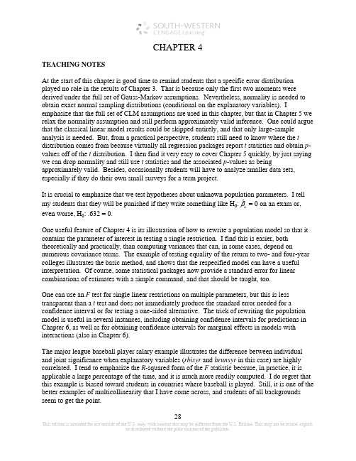
The Classical Linear Regression Model with one Incomplete Binary Variable

合集下载

机器学习试卷 mids14

y y
5
5
4
4
3
3
2
2
1
1
0
0
−1
−1
−2
−2
−3
−3
−4
−4
−5 −5 −4 −3 −2 −1
0
1
2
3
4
5
−5 −5 −4 −3 −2 −1
0
1
2
3
4
5
x
x
µ = [0, 0]T ,
10 Σ=
01
µ = [0, 1]T ,
40 Σ=
0 0.25
µ = [0, 1]T ,
10 Σ=
01
µ = [0, 1]T ,
L2
L∞
L1
None of the above
(f ) [3 pts] Suppose we have a covariance matrix
Σ=
5 a
a 4
What is the set of values that a can take on such that Σ is a valid covariance matrix?
Linear kernel Polynomial kernel
Gaussian RBF (radial basis function) kernel None of the above
(e) [3 pts] Consider the following plots of the contours of the unregularized error function along with the constraint region. What regularization term is used in this case?

计量经济学导论ch04习题答案

28CHAPTER 4TEACHING NOTESAt the start of this chapter is good time to remind students that a specific error distribution played no role in the results of Chapter 3. That is because only the first two moments were derived under the full set of Gauss-Markov assumptions. Nevertheless, normality is needed to obtain exact normal sampling distributions (conditional on the explanatory variables). Iemphasize that the full set of CLM assumptions are used in this chapter, but that in Chapter 5 we relax the normality assumption and still perform approximately valid inference. One could argue that the classical linear model results could be skipped entirely, and that only large-sample analysis is needed. But, from a practical perspective, students still need to know where the t distribution comes from because virtually all regression packages report t statistics and obtain p -values off of the t distribution. I then find it very easy to cover Chapter 5 quickly, by just saying we can drop normality and still use t statistics and the associated p -values as beingapproximately valid. Besides, occasionally students will have to analyze smaller data sets, especially if they do their own small surveys for a term project.It is crucial to emphasize that we test hypotheses about unknown population parameters. I tellmy students that they will be punished if they write something like H 0:1ˆβ = 0 on an exam or, even worse, H 0: .632 = 0.One useful feature of Chapter 4 is its illustration of how to rewrite a population model so that it contains the parameter of interest in testing a single restriction. I find this is easier, both theoretically and practically, than computing variances that can, in some cases, depend onnumerous covariance terms. The example of testing equality of the return to two- and four-year colleges illustrates the basic method, and shows that the respecified model can have a useful interpretation. Of course, some statistical packages now provide a standard error for linear combinations of estimates with a simple command, and that should be taught, too.One can use an F test for single linear restrictions on multiple parameters, but this is less transparent than a t test and does not immediately produce the standard error needed for aconfidence interval or for testing a one-sided alternative. The trick of rewriting the population model is useful in several instances, including obtaining confidence intervals for predictions in Chapter 6, as well as for obtaining confidence intervals for marginal effects in models with interactions (also in Chapter 6).The major league baseball player salary example illustrates the difference between individual and joint significance when explanatory variables (rbisyr and hrunsyr in this case) are highly correlated. I tend to emphasize the R -squared form of the F statistic because, in practice, it is applicable a large percentage of the time, and it is much more readily computed. I do regret that this example is biased toward students in countries where baseball is played. Still, it is one of the better examples of multicollinearity that I have come across, and students of all backgrounds seem to get the point.29SOLUTIONS TO PROBLEMS4.1 (i) H 0:3β = 0. H 1:3β > 0.(ii) The proportionate effect on n salaryis .00024(50) = .012. To obtain the percentage effect, we multiply this by 100: 1.2%. Therefore, a 50 point ceteris paribus increase in ros is predicted to increase salary by only 1.2%. Practically speaking, this is a very small effect for such a large change in ros .(iii) The 10% critical value for a one-tailed test, using df = ∞, is obtained from Table G.2 as 1.282. The t statistic on ros is .00024/.00054 ≈ .44, which is well below the critical value. Therefore, we fail to reject H 0 at the 10% significance level.(iv) Based on this sample, the estimated ros coefficient appears to be different from zero only because of sampling variation. On the other hand, including ros may not be causing any harm; it depends on how correlated it is with the other independent variables (although these are very significant even with ros in the equation).4.2 (i) and (iii) generally cause the t statistics not to have a t distribution under H 0.Homoskedasticity is one of the CLM assumptions. An important omitted variable violates Assumption MLR.3. The CLM assumptions contain no mention of the sample correlations among independent variables, except to rule out the case where the correlation is one.4.3 (i) While the standard error on hrsemp has not changed, the magnitude of the coefficient has increased by half. The t statistic on hrsemp has gone from about –1.47 to –2.21, so now the coefficient is statistically less than zero at the 5% level. (From Table G.2 the 5% critical value with 40 df is –1.684. The 1% critical value is –2.423, so the p -value is between .01 and .05.)(ii) If we add and subtract 2βlog(employ ) from the right-hand-side and collect terms, we havelog(scrap ) = 0β + 1βhrsemp + [2βlog(sales) – 2βlog(employ )] + [2βlog(employ ) + 3βlog(employ )] + u = 0β + 1βhrsemp + 2βlog(sales /employ ) + (2β + 3β)log(employ ) + u ,where the second equality follows from the fact that log(sales /employ ) = log(sales ) – log(employ ). Defining 3θ ≡ 2β + 3β gives the result.30(iii) No. We are interested in the coefficient on log(employ ), which has a t statistic of .2, which is very small. Therefore, we conclude that the size of the firm, as measured by employees, does not matter, once we control for training and sales per employee (in a logarithmic functional form).(iv) The null hypothesis in the model from part (ii) is H 0:2β = –1. The t statistic is [–.951 – (–1)]/.37 = (1 – .951)/.37 ≈ .132; this is very small, and we fail to reject whether we specify a one- or two-sided alternative.4.4 (i) In columns (2) and (3), the coefficient on profmarg is actually negative, although its t statistic is only about –1. It appears that, once firm sales and market value have been controlled for, profit margin has no effect on CEO salary.(ii) We use column (3), which controls for the most factors affecting salary. The t statistic on log(mktval ) is about 2.05, which is just significant at the 5% level against a two-sided alternative. (We can use the standard normal critical value, 1.96.) So log(mktval ) is statistically significant. Because the coefficient is an elasticity, a ceteris paribus 10% increase in market value is predicted to increase salary by 1%. This is not a huge effect, but it is not negligible, either.(iii) These variables are individually significant at low significance levels, with t ceoten ≈ 3.11 and t comten ≈ –2.79. Other factors fixed, another year as CEO with the company increases salary by about 1.71%. On the other hand, another year with the company, but not as CEO, lowers salary by about .92%. This second finding at first seems surprising, but could be related to the “superstar” effect: firms that hire CEOs from outside the company often go after a small pool of highly regarded candidates, and salaries of these people are bid up. More non-CEO years with a company makes it less likely the person was hired as an outside superstar.4.5 (i) With df = n – 2 = 86, we obtain the 5% critical value from Table G.2 with df = 90.Because each test is two-tailed, the critical value is 1.987. The t statistic for H 0:0β = 0 is about -.89, which is much less than 1.987 in absolute value. Therefore, we fail to reject 0β = 0. The t statistic for H 0: 1β = 1 is (.976 – 1)/.049 ≈ -.49, which is even less significant. (Remember, we reject H 0 in favor of H 1 in this case only if |t | > 1.987.)(ii) We use the SSR form of the F statistic. We are testing q = 2 restrictions and the df in the unrestricted model is 86. We are given SSR r = 209,448.99 and SSR ur = 165,644.51. Therefore,(209,448.99165,644.51)8611.37,165,644.512F −⎛⎞=⋅≈⎜⎟⎝⎠which is a strong rejection of H 0: from Table G.3c, the 1% critical value with 2 and 90 df is 4.85.31(iii) We use the R -squared form of the F statistic. We are testing q = 3 restrictions and there are 88 – 5 = 83 df in the unrestricted model. The F statistic is [(.829 – .820)/(1 – .829)](83/3) ≈ 1.46. The 10% critical value (again using 90 denominator df in Table G.3a) is 2.15, so we fail to reject H 0 at even the 10% level. In fact, the p -value is about .23.(iv) If heteroskedasticity were present, Assumption MLR.5 would be violated, and the F statistic would not have an F distribution under the null hypothesis. Therefore, comparing the F statistic against the usual critical values, or obtaining the p -value from the F distribution, would not be especially meaningful.4.6 (i) We need to compute the F statistic for the overall significance of the regression with n = 142 and k = 4: F = [.0395/(1 – .0395)](137/4) ≈ 1.41. The 5% critical value with 4 numerator df and using 120 for the numerator df , is 2.45, which is well above the value of F . Therefore, we fail to reject H 0: 1β = 2β = 3β = 4β = 0 at the 10% level. No explanatory variable isindividually significant at the 5% level. The largest absolute t statistic is on dkr , t dkr ≈ 1.60, which is not significant at the 5% level against a two-sided alternative.(ii) The F statistic (with the same df ) is now [.0330/(1 – .0330)](137/4) ≈ 1.17, which is even lower than in part (i). None of the t statistics is significant at a reasonable level.(iii) We probably should not use the logs, as the logarithm is not defined for firms that have zero for dkr or eps . Therefore, we would lose some firms in the regression.(iv) It seems very weak. There are no significant t statistics at the 5% level (against a two-sided alternative), and the F statistics are insignificant in both cases. Plus, less than 4% of the variation in return is explained by the independent variables.4.7 (i) .412 ± 1.96(.094), or about .228 to .596.(ii) No, because the value .4 is well inside the 95% CI.(iii) Yes, because 1 is well outside the 95% CI.4.8 (i) With df = 706 – 4 = 702, we use the standard normal critical value (df = ∞ in Table G.2), which is 1.96 for a two-tailed test at the 5% level. Now t educ = −11.13/5.88 ≈ −1.89, so |t educ | = 1.89 < 1.96, and we fail to reject H 0: educ β = 0 at the 5% level. Also, t age ≈ 1.52, so age is also statistically insignificant at the 5% level.(ii) We need to compute the R -squared form of the F statistic for joint significance. But F = [(.113 − .103)/(1 − .113)](702/2) ≈ 3.96. The 5% critical value in the F 2,702 distribution can be obtained from Table G.3b with denominator df = ∞: cv = 3.00. Therefore, educ and age are jointly significant at the 5% level (3.96 > 3.00). In fact, the p -value is about .019, and so educ and age are jointly significant at the 2% level.32(iii) Not really. These variables are jointly significant, but including them only changes the coefficient on totwrk from –.151 to –.148.(iv) The standard t and F statistics that we used assume homoskedasticity, in addition to the other CLM assumptions. If there is heteroskedasticity in the equation, the tests are no longer valid.4.9 (i) H 0:3β = 0. H 1:3β ≠ 0.(ii) Other things equal, a larger population increases the demand for rental housing, which should increase rents. The demand for overall housing is higher when average income is higher, pushing up the cost of housing, including rental rates.(iii) The coefficient on log(pop ) is an elasticity. A correct statement is that “a 10% increase in population increases rent by .066(10) = .66%.”(iv) With df = 64 – 4 = 60, the 1% critical value for a two-tailed test is 2.660. The t statistic is about 3.29, which is well above the critical value. So 3β is statistically different from zero at the 1% level.4.10 (i) We use Property VAR.3 from Appendix B: Var(1ˆβ − 32ˆβ) = Var (1ˆβ) + 9 Var (2ˆβ) – 6 Cov (1ˆβ,2ˆβ).(ii) t = (1ˆβ− 32ˆβ − 1)/se(1ˆβ− 32ˆβ), so we need the standard error of 1ˆβ − 32ˆβ.(iii) Because1θ = 1β – 3β2, we can write 1β = 1θ + 3β2. Plugging this into the population model gives y = 0β + (1θ + 3β2)x 1 + 2βx 2 + 3βx 3 + u = 0β + 1θx 1 + 2β(3x 1 + x 2) + 3βx 3 + u .This last equation is what we would estimate by regressing y on x 1, 3x 1 + x 2, and x 3. The coefficient and standard error on x 1 are what we want.4.11 (i) Holding profmarg fixed, n rdintensΔ = .321 Δlog(sales ) = (.321/100)[100log()sales ⋅Δ] ≈ .00321(%Δsales ). Therefore, if %Δsales = 10, n rdintens Δ ≈ .032, or only about 3/100 of a percentage point. For such a large percentage increase in sales,this seems like a practically small effect.33(ii) H 0:1β = 0 versus H 1:1β > 0, where 1β is the population slope on log(sales ). The t statistic is .321/.216 ≈ 1.486. The 5% critical value for a one-tailed test, with df = 32 – 3 = 29, is obtained from Table G.2 as 1.699; so we cannot reject H 0 at the 5% level. But the 10% critical value is 1.311; since the t statistic is above this value, we reject H 0 in favor of H 1 at the 10% level.(iii) Not really. Its t statistic is only 1.087, which is well below even the 10% critical value for a one-tailed test.34SOLUTIONS TO COMPUTER EXERCISESC4.1 (i) Holding other factors fixed,111log()(/100)[100log()](/100)(%),voteA expendA expendA expendA βββΔ=Δ=⋅Δ≈Δwhere we use the fact that 100log()expendA ⋅Δ ≈ %expendA Δ. So 1β/100 is the (ceteris paribus) percentage point change in voteA when expendA increases by one percent.(ii) The null hypothesis is H 0: 2β = –1β, which means a z% increase in expenditure by A and a z% increase in expenditure by B leaves voteA unchanged. We can equivalently write H 0: 1β + 2β = 0.(iii) The estimated equation (with standard errors in parentheses below estimates) isn voteA = 45.08 + 6.083 log(expendA ) – 6.615 log(expendB ) + .152 prtystrA (3.93) (0.382) (0.379) (.062)n = 173, R 2 = .793.The coefficient on log(expendA ) is very significant (t statistic ≈ 15.92), as is the coefficient on log(expendB ) (t statistic ≈ –17.45). The estimates imply that a 10% ceteris paribus increase in spending by candidate A increases the predicted share of the vote going to A by about .61percentage points. [Recall that, holding other factors fixed, n voteAΔ≈(6.083/100)%ΔexpendA ).] Similarly, a 10% ceteris paribus increase in spending by B reduces n voteAby about .66 percentage points. These effects certainly cannot be ignored.While the coefficients on log(expendA ) and log(expendB ) are of similar magnitudes (andopposite in sign, as we expect), we do not have the standard error of 1ˆβ + 2ˆβ, which is what we would need to test the hypothesis from part (ii).(iv) Write1θ = 1β +2β, or 1β = 1θ– 2β. Plugging this into the original equation, and rearranging, givesn voteA = 0β + 1θlog(expendA ) + 2β[log(expendB ) – log(expendA )] +3βprtystrA + u ,When we estimate this equation we obtain 1θ≈ –.532 and se( 1θ)≈ .533. The t statistic for the hypothesis in part (ii) is –.532/.533 ≈ –1. Therefore, we fail to reject H 0: 2β = –1β.35C4.2 (i) In the modellog(salary ) = 0β+1βLSAT +2βGPA + 3βlog(libvol ) +4βlog(cost)+5βrank + u ,the hypothesis that rank has no effect on log(salary ) is H 0:5β = 0. The estimated equation (now with standard errors) isn log()salary = 8.34 + .0047 LSAT + .248 GPA + .095 log(libvol )(0.53) (.0040) (.090) (.033)+ .038 log(cost ) – .0033 rank (.032) (.0003)n = 136, R 2 = .842.The t statistic on rank is –11, which is very significant. If rank decreases by 10 (which is a move up for a law school), median starting salary is predicted to increase by about 3.3%.(ii) LSAT is not statistically significant (t statistic ≈ 1.18) but GPA is very significance (t statistic ≈ 2.76). The test for joint significance is moot given that GPA is so significant, but for completeness the F statistic is about 9.95 (with 2 and 130 df ) and p -value ≈ .0001.(iii) When we add clsize and faculty to the regression we lose five observations. The test of their joint significant (with 2 and 131 – 8 = 123 df ) gives F ≈ .95 and p -value ≈ .39. So these two variables are not jointly significant unless we use a very large significance level.(iv) If we want to just determine the effect of numerical ranking on starting law school salaries, we should control for other factors that affect salaries and rankings. The idea is that there is some randomness in rankings, or the rankings might depend partly on frivolous factors that do not affect quality of the students. LSAT scores and GPA are perhaps good controls for student quality. However, if there are differences in gender and racial composition acrossschools, and systematic gender and race differences in salaries, we could also control for these. However, it is unclear why these would be correlated with rank . Faculty quality, as perhaps measured by publication records, could be included. Such things do enter rankings of law schools.C4.3 (i) The estimated model isn log()price = 11.67 + .000379 sqrft + .0289 bdrms (0.10) (.000043) (.0296)n = 88, R 2 = .588.36Therefore, 1ˆθ= 150(.000379) + .0289 = .0858, which means that an additional 150 square foot bedroom increases the predicted price by about 8.6%.(ii)2β= 1θ – 1501β, and solog(price ) = 0β+ 1βsqrft + (1θ – 1501β)bdrms + u=0β+ 1β(sqrft – 150 bdrms ) + 1θbdrms + u .(iii) From part (ii), we run the regressionlog(price ) on (sqrft – 150 bdrms ), bdrms ,and obtain the standard error on bdrms . We already know that 1ˆθ= .0858; now we also getse(1ˆθ) = .0268. The 95% confidence interval reported by my software package is .0326 to .1390(or about 3.3% to 13.9%).C4.4 The R -squared from the regression bwght on cigs , parity , and faminc , using all 1,388observations, is about .0348. This means that, if we mistakenly use this in place of .0364, which is the R -squared using the same 1,191 observations available in the unrestricted regression, we would obtain F = [(.0387 − .0348)/(1 − .0387)](1,185/2) ≈ 2.40, which yields p -value ≈ .091 in an F distribution with 2 and 1,1185 df . This is significant at the 10% level, but it is incorrect. The correct F statistic was computed as 1.42 in Example 4.9, with p -value ≈ .242.C4.5 (i) If we drop rbisyr the estimated equation becomesn log()salary = 11.02 + .0677 years + .0158 gamesyr (0.27) (.0121) (.0016) + .0014 bavg + .0359 hrunsyr (.0011) (.0072)n = 353, R 2= .625.Now hrunsyr is very statistically significant (t statistic ≈ 4.99), and its coefficient has increased by about two and one-half times.(ii) The equation with runsyr , fldperc , and sbasesyr added is37n log()salary = 10.41 + .0700 years + .0079 gamesyr(2.00) (.0120) (.0027)+ .00053 bavg + .0232 hrunsyr(.00110) (.0086)+ .0174 runsyr + .0010 fldperc – .0064 sbasesyr (.0051) (.0020) (.0052) n = 353, R 2 = .639.Of the three additional independent variables, only runsyr is statistically significant (t statistic = .0174/.0051 ≈ 3.41). The estimate implies that one more run per year, other factors fixed,increases predicted salary by about 1.74%, a substantial increase. The stolen bases variable even has the “wrong” sign with a t statistic of about –1.23, while fldperc has a t statistic of only .5. Most major league baseball players are pretty good fielders; in fact, the smallest fldperc is 800 (which means .800). With relatively little variation in fldperc , it is perhaps not surprising that its effect is hard to estimate.(iii) From their t statistics, bavg , fldperc , and sbasesyr are individually insignificant. The F statistic for their joint significance (with 3 and 345 df ) is about .69 with p -value ≈ .56. Therefore, these variables are jointly very insignificant.C4.6 (i) In the modellog(wage ) = 0β + 1βeduc + 2βexper + 3βtenure + uthe null hypothesis of interest is H 0: 2β = 3β.(ii) Let2θ = 2β – 3β. Then we can estimate the equationlog(wage ) = 0β + 1βeduc + 2θexper + 3β(exper + tenure ) + uto obtain the 95% CI for 2θ. This turns out to be about .0020 ± 1.96(.0047), or about -.0072 to .0112. Because zero is in this CI, 2θ is not statistically different from zero at the 5% level, and we fail to reject H 0: 2β = 3β at the 5% level.C4.7 (i) The minimum value is 0, the maximum is 99, and the average is about 56.16. (ii) When phsrank is added to (4.26), we get the following:n log() wage = 1.459 − .0093 jc + .0755 totcoll + .0049 exper + .00030 phsrank (0.024) (.0070) (.0026) (.0002) (.00024)38 n = 6,763, R 2 = .223So phsrank has a t statistic equal to only 1.25; it is not statistically significant. If we increase phsrank by 10, log(wage ) is predicted to increase by (.0003)10 = .003. This implies a .3% increase in wage , which seems a modest increase given a 10 percentage point increase in phsrank . (However, the sample standard deviation of phsrank is about 24.)(iii) Adding phsrank makes the t statistic on jc even smaller in absolute value, about 1.33, but the coefficient magnitude is similar to (4.26). Therefore, the base point remains unchanged: the return to a junior college is estimated to be somewhat smaller, but the difference is not significant and standard significant levels.(iv) The variable id is just a worker identification number, which should be randomly assigned (at least roughly). Therefore, id should not be correlated with any variable in the regression equation. It should be insignificant when added to (4.17) or (4.26). In fact, its t statistic is about .54.C4.8 (i) There are 2,017 single people in the sample of 9,275.(ii) The estimated equation isn nettfa = −43.04 + .799 inc + .843 age ( 4.08) (.060) (.092)n = 2,017, R 2 = .119.The coefficient on inc indicates that one more dollar in income (holding age fixed) is reflected in about 80 more cents in predicted nettfa ; no surprise there. The coefficient on age means that, holding income fixed, if a person gets another year older, his/her nettfa is predicted to increase by about $843. (Remember, nettfa is in thousands of dollars.) Again, this is not surprising.(iii) The intercept is not very interesting as it gives the predicted nettfa for inc = 0 and age = 0. Clearly, there is no one with even close to these values in the relevant population.(iv) The t statistic is (.843 − 1)/.092 ≈ −1.71. Against the one-sided alternative H 1: β2 < 1, the p-value is about .044. Therefore, we can reject H 0: β2 = 1 at the 5% significance level (against the one-sided alternative).(v) The slope coefficient on inc in the simple regression is about .821, which is not very different from the .799 obtained in part (ii). As it turns out, the correlation between inc and age in the sample of single people is only about .039, which helps explain why the simple and multiple regression estimates are not very different; refer back to page 84 of the text.39C4.9 (i) The results from the OLS regression, with standard errors in parentheses, aren log() psoda =−1.46 + .073 prpblck + .137 log(income ) + .380 prppov (0.29) (.031) (.027) (.133)n = 401, R 2 = .087The p -value for testing H 0: 10β= against the two-sided alternative is about .018, so that wereject H 0 at the 5% level but not at the 1% level.(ii) The correlation is about −.84, indicating a strong degree of multicollinearity. Yet eachcoefficient is very statistically significant: the t statistic for log()ˆincome β is about 5.1 and that forˆprppovβ is about 2.86 (two-sided p -value = .004).(iii) The OLS regression results when log(hseval ) is added aren log() psoda =−.84 + .098 prpblck − .053 log(income ) (.29) (.029) (.038)+ .052 prppov + .121 log(hseval )(.134) (.018)n = 401, R 2 = .184The coefficient on log(hseval ) is an elasticity: a one percent increase in housing value, holding the other variables fixed, increases the predicted price by about .12 percent. The two-sided p -value is zero to three decimal places.(iv) Adding log(hseval ) makes log(income ) and prppov individually insignificant (at even the 15% significance level against a two-sided alternative for log(income ), and prppov is does not have a t statistic even close to one in absolute value). Nevertheless, they are jointly significant at the 5% level because the outcome of the F 2,396 statistic is about 3.52 with p -value = .030. All of the control variables – log(income ), prppov , and log(hseval ) – are highly correlated, so it is not surprising that some are individually insignificant.(v) Because the regression in (iii) contains the most controls, log(hseval ) is individually significant, and log(income ) and prppov are jointly significant, (iii) seems the most reliable. It holds fixed three measure of income and affluence. Therefore, a reasonable estimate is that if the proportion of blacks increases by .10, psoda is estimated to increase by 1%, other factors held fixed.40C4.10 (i) Using the 1,848 observations, the simple regression estimate of bs β is about .795−. The 95% confidence interval runs from 1.088 to .502−−, which includes −1. Therefore, at the 5% level, we cannot reject that 0H :1bs β=− against the two-sided alternative.(ii) When lenrol and lstaff are added to the regression, the coefficient on bs becomes about −.605; it is now statistically different from one, as the 95% CI is from about −.818 to −.392. The situation is very similar to that in Table 4.1, where the simple regression estimate is −.825 and the multiple regression estimate (with the logs of enrollment and staff included) is −.605. (It is a coincidence that the two multiple regression estimates are the same, as the data set in Table 4.1 is for an earlier year at the high school level.)(iii) The standard error of the simple regression estimate is about .150, and that for the multiple regression estimate is about .109. When we add extra explanatory variables, two factors work in opposite directions on the standard errors. Multicollinearity – in this case, correlation between bs and the two variables lenrol and lstaff works to increase the multiple regressionstandard error. Working to reduce the standard error of ˆbsβis the smaller error variance when lenrol and lstaff are included in the regression; in effect, they are taken out of the simpleregression error term. In this particular example, the multicollinearity is modest compared with the reduction in the error variance. In fact, the standard error of the regression goes from .231 for simple regression to .168 in the multiple regression. (Another way to summarize the drop in the error variance is to note that the R -squared goes from a very small .0151 for the simpleregression to .4882 for multiple regression.) Of course, ahead of time we cannot know which effect will dominate, but we can certainly compare the standard errors after running both regressions.(iv) The variable lstaff is the log of the number of staff per 1,000 students. As lstaff increases, there are more teachers per student. We can associate this with smaller class sizes, which are generally desirable from a teacher’s perspective. It appears that, all else equal, teachers are willing to take less in salary to have smaller class sizes. The elasticity of salary with respect to staff is about −.714, which seems quite large: a ten percent increase in staff size (holding enrollment fixed) is associated with a 7.14 percent lower salary.(v) When lunch is added to the regression, its coefficient is about −.00076, with t = −4.69. Therefore, other factors fixed (bs , lenrol , and lstaff ), a hire poverty rate is associated with lower teacher salaries. In this data set, the average value of lunch is about 36.3 with standard deviation of 25.4. Therefore, a one standard deviation increase in lunch is associated with a change in lsalary of about −.00076(25.4) ≈ −.019, or almost two percent lower. Certainly there is no evidence that teachers are compensated for teaching disadvantaged children.(vi) Yes, the pattern obtained using ELEM94_95.RAW is very similar to that in Table 4.1, and the magnitudes are reasonably close, too. The largest estimate (in absolute value) is the simple regression estimate, and the absolute value declines as more explanatory variables are added. The final regressions in the two cases are not the same, because we do not control for lunch in Table 4.1, and graduation and dropout rates are not relevant for elementary school children.。

SimTimeVar 1.0.0 软件包说明说明书

Package‘SimTimeVar’October12,2022Type PackageTitle Simulate Longitudinal Dataset with Time-Varying CorrelatedCovariatesVersion1.0.0Date2017-09-07AuthorMaya B.Mathur,Kristopher Kapphahn,Ariadna Garcia,Manisha Desai,Maria E.Montez-Rath Maintainer Maya B.Mathur<********************>Description Flexibly simulates a dataset with time-varying covariates with user-speciﬁed exchange-able correlation structures across and within clusters.Covariates can be normal or bi-nary and can be static within a cluster or time-varying.Time-varying normal variables can op-tionally have linear trajectories within each cluster.See?make_one_dataset for the main wrap-per function.See Montez-Rath et al.<arXiv:1709.10074>for methodological details. LazyData trueLicense GPL-2Imports metafor,mvtnorm,ICC,miscTools,car,plyr,corpcor,psych,stats,utilsRoxygenNote6.0.1NeedsCompilation noRepository CRANDate/Publication2017-09-3016:22:10UTCR topics documented:add_one_categorical (2)add_time_function_vars (3)BN.rBound (3)cat.params (4)closest (4)complete_parameters (5)expand_matrix (5)12add_one_categorical expand_subjects (6)has_drug_sufﬁx (7)make_one_dataset (7)make_one_linear_pred (9)mod.jointly.generate.binary.normal (10)override_static (11)override_tbin_probs (11)params (12)pcor (12)proportionize (13)upper_tri_vec (13)wcor (14)Index15 add_one_categorical Generate linear predictor from logistic modelDescriptionAn internal function not intended for the user.Given a dataset and multinomial regression parame-ters,generates a categorical variable and adds it to the dataset.Usageadd_one_categorical(.d,n,obs,cat.parameters)Arguments.d The dataset to which to add the categorical variable.n The number of clusters.obs The number of observations per cluster.cat.parameters A dataframe of parameters for generating the categorical variable.See Details.Examples#mini dataset with3observations per persondata=data.frame(male=rep(rbinom(n=10,size=1,prob=0.5),each=3))add_one_categorical(data,10,3,cat.params)add_time_function_vars3add_time_function_varsCreates linear time-function variablesDescriptionGiven variable-speciﬁc slopes and intercepts for a cluster,creates continuous variables that increase or decrease linearly in time(with normal error with standard deviation error.SD)and adds them to the dataframe.Usageadd_time_function_vars(d4,obs,parameters)Argumentsd4The dataframe to which to add the time-function variables.obs The number of observations per cluster.parameters The parameters matrix.DetailsSee make_one_dataset for additional information.BN.rBound Maximum correlation between binary and normal random variablesDescriptionGiven parameter p for a Bernoulli random variable,returns its maximum possible correlation with an arbitrary normal random ed to adjust correlation matrices whose entries are not theoretically possible.UsageBN.rBound(p)Argumentsp Parameter of Bernoulli random variable.Examples#find the largest possible correlation between a normal#variable and a binary with parameter0.1BN.rBound(0.1)4closest cat.params An example dataframe for categorical variable parametersDescriptionAn example of how to set up the categorical variable parameters dataframe.Usagecat.paramsFormatAn object of class data.frame with5rows and3columns.closest Return closest valueDescriptionAn internal function not intended for the user.Given a number x and vector of permitted values, returns the closest permitted value to x(in absolute value).Usageclosest(x,candidates)Argumentsx The number to be compared to the permitted values.candidates A vector of permitted values.Examplesclosest(x=5,candidates=c(-3,8,25))complete_parameters5 complete_parameters Fill in partially incomplete parameters matrixDescriptionFills in"strategic"NA values in a user-provided parameters matrix by(1)calculating SDs for pro-portions using the binomial distribution;(2)calculating variances based on SDs;and(3)setting within-cluster variances to1/3of the across-cluster variances(if not already speciﬁed).Usagecomplete_parameters(parameters,n)Argumentsparameters Initial parameters matrix that may contain NA values.n The number of clustersDetailsFor binary variables,uses binomial distribution to compute across-cluster standard deviation of proportion.Where there are missing values,ﬁlls in variances given standard deviations and vice-versa.Where there are missing values in within.var,ﬁlls these in by defaulting to1/3of the corresponding across-cluster variance.Examplescomplete_parameters(params,n=10)expand_matrix Longitudinally expand a matrix of single observations by clusterDescriptionAn internal function not intended for the user.Given a matrix of single observations for a cluster, repeats each cluster’s entry in each.obs times.Usageexpand_matrix(.matrix,.obs)Arguments.matrix The matrix of observations to be expanded..obs The number of observations to generate per cluster.6expand_subjectsExamplesmat=matrix(seq(1:10),nrow=2,byrow=FALSE)expand_matrix(mat,4)expand_subjects Longitudinally expand a clusterDescriptionAn internal function not intended for the user.Given a matrix of cluster means for each variable to be simulated,"expands"them into time-varying observations.Usageexpand_subjects(mus3,n.OtherNorms,n.OtherBins,n.TBins,wcor,obs,parameters, zero=1e-04)Argumentsmus3A matrix of cluster means for each variable.n.OtherNorms The number normal variables(not counting those used for generating a time-varying binary variable).n.OtherBins The number of static binary variables.n.TBins The number of time-varying binary variables.wcor The within-cluster correlation matrix.obs The number of observations to generate per cluster.parameters The parameters dataframe.zero A small number just larger than0.Examples#subject means matrix(normally would be created internally within make_one_dataset) mus3=structure(c(1,0,1,0,0,0,1,1,1,1,1e-04,1e-04,0.886306145591761,1e-04,1e-04,1e-04,1e-04,0.875187001140343,0.835990583043838,1e-04,1e-04,1e-04,1e-04,1e-04,1e-04,1e-04,1e-04,1e-04,1e-04,1e-04,69.7139993804559,61.3137637852213,68.3375516615242,57.7893277997516,66.3744152975352,63.7829561873355,66.3864252981679,68.8513253460358,67.4120718557,67.8332265185068,192.366192293195,128.048983102048,171.550401133259,120.348392753954,158.840864356998,170.134********,113.512220330821,162.715528382999,138.476877345895,159.841096973242,115.026417822477,109.527137142158,117.0879********,121.153861460319,109.95973584141,122.96960673409,90.5100006255084,107.523229006601,108.971677388246,115.641818648526,-4.33184270434101,-5.45143483618415,-2.56331188314257,-1.38204452333064,-1.61744564863871,1.83911233741448,2.0488338883998,-0.237095062415858,-5.47497506857878,-3.53078955238741),.Dim=c(10L,7L))has_drug_sufﬁx7 expand_subjects(mus3=mus3,n.OtherNorms=4,n.OtherBins=1,n.TBins=2,wcor=wcor,obs=3,parameters=complete_parameters(params,n=10)) has_drug_suffix Checks whether string has"_s"sufﬁxDescriptionAn internal function not intended for the user.Usagehas_drug_suffix()Arguments The string to be checkedExampleshas_drug_suffix("myvariable_s")has_drug_suffix("myvariable")make_one_dataset Simulate time-varying covariatesDescriptionSimulates a dataset with correlated time-varying covariates with an exchangeable correlation struc-ture.Covariates can be normal or binary and can be static within a cluster or time-varying.Time-varying normal variables can optionally have linear trajectories within each cluster.Usagemake_one_dataset(n,obs,n.TBins,pcor,wcor,parameters,cat.parameters) Argumentsn The number of clusters.obs The number of observations per cluster.n.TBins Number of time-varying binary variables.pcor The across-subject correlation matrix.See Details.wcor The within-subject correlation matrix.See Details.parameters A dataframe containing the general simulation parameters.See Details.cat.parameters A dataframe containing parameters for the categorical variables.See Details.8make_one_dataset DetailsSPECIFYING THE PARAMETERS MATRIXThe matrix parameters contains parameters required to generate all non-categorical variables.It must contain column names name,type,across.mean,across.SD,across.var,within.var, prop,and error.SD.(To see an example,use data(params).)Each variable to be generated re-quires either one or two rows in parameters,depending on the variable type.The possible variable types and their corresponding speciﬁcations are:•Static binary variables do not change over time within a cluster.For example,if clusters are subjects,sex would be a static binary variable.Generating such a variable requires a single row of type static.binary with prop corresponding to the proportion of clusters for which the variable equals1and all other columns set to NA.(The correct standard deviation will automatically be computed later.)For example,if the variable is an indicator for a subject’s being male,then prop speciﬁes the proportion of males to be generated.•Time-varying binary variables can change within a cluster over time,as for an indicator for whether a subject is currently taking the study drug.These variables require two rows in parameters.Theﬁrst row should be of type static.binary with prop representing the proportion of clusters for which the time-varying binary variable is1at least once(and all other columns set to NA).For example,this row in parameters could represent the proportion of subjects who ever take the study drug("ever-users").The second row should be of type subject.prop with across.mean representing,for clusters that ever have a1for the binary variable,the proportion of observations within the cluster for which the variable is equal to1.(All other columns should be set to NA.)For example,this this row in parameters could represent the proportion of observations for which an ever-user is currently taking the drug.To indicate which pair of variables go together,the subject.prop should have the same name as the static.binary variable,but with the sufﬁx_s appended (for example,the former could be named drug_s and the latter drug).•Normal variables are normally distributed within a cluster such that the within-cluster means are themselves also normally distributed in the population of clusters.Generating a normal variable requires speciﬁcation of the population mean(across.mean)and standard deviation (across.SD)as well as of the within-cluster standard deviation(within.SD).To generate a static continuous variable,simply set within.SD to be extremely small(e.g.,$1*10^-7$)and all corresponding correlations in matrix wcor to0.•Time-function variables are linear functions of time(with normal error)within each cluster such that the within-cluster baseline values are normally distributed in the population of clus-ters.Generating a time-function variable requires two entries.Theﬁrst entry should be of type time.function and speciﬁes the population mean(across.mean)and standard devia-tion(across.SD)of the within-cluster baseline values as well as the error standard deviation (error.SD).The second entry should be of type normal and should have the same name as the time.function entry,but with the"_s"sufﬁx.This entry speciﬁes the mean(across.mean) and standard deviation(across.SD)of the within-cluster slopes.SPECIFYING THE CATEGORICAL PARAMETERS MATRIXThe matrix cat.parameters contains parameters required to generate the single categorical vari-able,if any.It must contain column names level,parameter,and beta.(To see an example,use data(cat.params).)make_one_linear_pred9•The reference level:Each categorical variable must have exactly one"reference"level.The reference level should have one row in cat.parameters for which parameters is set to NA and beta is set to ref.For example,in the exampleﬁle cat.params specifying parameters to generate a subject’s race,the reference level is white.•Other levels:Other levels of the categorical variable will have one or more rows.One row with parameter set to intercept and beta set to a numeric value represents the intercept term in the corresponding multinomial model.Any subsequent rows,with parameters set to names of other variables in the dataset and beta set to numeric values,represents other coefﬁcients in the corresponding multinomial models.SPECIFYING THE POPULATION CORRELATION MATRIXMatrix pcor speciﬁes the population(i.e.,across-cluster)correlation matrix.It should have the same number of rows and columns as parameters as well as the same variable names and ordering of variables.SPECIFYING THE WITHIN-CLUSTER CORRELATION MATRIXMatrix wcor speciﬁes the within-cluster correlation matrix.The order of the variables listed in thisﬁle should be consistent with the order in params and pcor.However,static.binary and subject.prop variables should not be included in wcor since they are static within a cluster.Static continuous variables should be included,but all the correlations should be set to zero.Examplesdata=make_one_dataset(n=10,obs=10,n.TBins=2,pcor=pcor,wcor=wcor,parameters=complete_parameters(params,n=10),cat.parameters=cat.params)$datamake_one_linear_pred Generate linear predictor from logistic modelDescriptionAn internal function not intended for the user.Given a matrix of regression parameters and a dataset, returns the linear predictor based on the given dataset.Usagemake_one_linear_pred(m,data)Argumentsm Part of the parameter matrix for the linear predictor for a single variable.data The dataframe from which to generate.10mod.jointly.generate.binary.normal Examples#take part of parameters matrix corresponding to single level of categorical#variablem=cat.params[cat.params$level=="black",]data=data.frame(male=rbinom(n=10,size=1,prob=0.5))make_one_linear_pred(m,data)mod.jointly.generate.binary.normalReturn closest valueDescriptionAn internal function not intended for the user.Simulates correlated normal and binary variables based on the algorithm of Demirtas and Doganay(2012).See references for further information. Usagemod.jointly.generate.binary.normal(no.rows,no.bin,no.nor,prop.vec.bin,mean.vec.nor,var.nor,corr.vec,adjust.corrs=TRUE)Argumentsno.rows Number of rowsno.bin Number of binary variablesno.nor Number of normal variablesprop.vec.bin Vector of parameters for binary variablesmean.vec.nor Vector of means for binary variablesvar.nor Vector of variances for binary variablescorr.vec Vector of correlationsadjust.corrs Boolean indicating whether theoretically impossible correlations between a bi-nary and a normal variable should be adjusted to their closest theoretically pos-sible value.ReferencesDemirtas,H.,&Doganay,B.(2012).Simultaneous generation of binary and normal data with speciﬁed marginal and association structures.Journal of Biopharmaceutical Statistics,22(2),223-236.override_static11 override_static Override static variableDescriptionAn internal function not intended for the user.For static variables,overrides any time-varying values to ensure that they are actually static.Usageoverride_static(,="id",.d,.obs)ArgumentsName of static variable. Name of variable deﬁning clusters in dataset..d Dataset.obs The number of observations per cluster.Examples#example with10subjects each with3observations#generate sex in a way where it might vary within a subjectdata=data.frame(id=rep(1:10,each=3),male=rbinom(n=10*3,size=1,prob=0.5))override_static("male","id",data,3)override_tbin_probs Override probabilities for time-varying binary variablesDescriptionAn internal function not intended for the user.For clusters assigned to have a given time-varying binary variable always equal to0,overrides to0the corresponding proportion of observations with the binary variable equal to1.Usageoverride_tbin_probs(mus0,n.TBins,n.OtherBins,zero=1e-04)Argumentsmus0The matrix of cluster means.n.TBins Number of time-varying binary variables.n.OtherBins The number of static binary variables.zero A number very close to0,but slightly larger.12pcorExamples#make example subject means matrix for1static binary,#1time-varying binary,and1normal#50subjects and5observations(latter plays into variance)set.seed(451)mus0=mod.jointly.generate.binary.normal(no.rows=50,no.bin=2,no.nor=2,prop.vec.bin=c(.5,.35),mean.vec.nor=c(.4,100),var.nor=c((0.4*0.6)/5,10),corr.vec=c(0.05,.08,0,0,-0.03,0))#note that we have ever-users with non-zero propensities to be on drug:not okayany(mus0[,1]==0&mus0[,3]!=0)#fix themmus1=override_tbin_probs(mus0,1,1)#all better!any(mus1[,1]==0&mus1[,3]>0.0001)params An example parameters dataframeDescriptionAn example of how to set up the parameters dataframe.UsageparamsFormatAn object of class data.frame with12rows and8columns.pcor An example across-cluster correlation dataframeDescriptionAn example of how to set up the across-cluster correlation dataframe.UsagepcorFormatAn object of class data.frame with9rows and9columns.proportionize13 proportionize Turn a number into a valid proportionDescriptionAn internal function not intended for the user.Turns an arbitrary number into a valid proportion by setting the number equal to the closest value in[0,1].Usageproportionize(x,zero=1e-05,one=0.999)Argumentsx The number to be turned into a proportion.zero A very small number that is just larger than0.one A number that is just smaller than1.Examplesproportionize(-0.03)proportionize(1.2)proportionize(.63)upper_tri_vec Turn symmetric matrix into vectorDescriptionAn internal function not intended for the user.Turns a matrix into a vector of the upper-triangular elements(arranged by row).Usageupper_tri_vec(m)Argumentsm MatrixExamples#make a simple correlation matrixx=rnorm(10);y=rnorm(10);z=rnorm(10)mat=cor(data.frame(x,y,z))#turn into into vectorupper_tri_vec(mat)14wcor wcor An example within-cluster correlation dataframeDescriptionAn example of how to set up the within-cluster correlation dataframe.UsagewcorFormatAn object of class data.frame with6rows and6columns.Index∗datasetscat.params,4params,12pcor,12wcor,14add_one_categorical,2add_time_function_vars,3BN.rBound,3cat.params,4closest,4complete_parameters,5expand_matrix,5expand_subjects,6has_drug_suffix,7make_one_dataset,7make_one_linear_pred,9mod.jointly.generate.binary.normal,10 override_static,11override_tbin_probs,11params,12pcor,12proportionize,13upper_tri_vec,13wcor,1415。

经典线性回归模型

·β的OLS估计量：在假定2.3成立时
( ) å å b =
XTX
-1 X T Y
= çæ 1 èn
n i=1
xi xiT
Hale Waihona Puke -1ö æ1 ÷ç ø èn
n i=1
xi yi
÷ö ø
( ) ·估计量的抽样误差（sampling error）： b - b = X T X -1 X Te
·第i次观测的拟合值（fitted value）： yˆi = xiTb
且自变量的回归系数和 y 与 x 的样本相关系数之间的关系为
b1 == corr(Y , X )
å( 1 n
n - 1 i=1
yi
- y)2
º r sy
å( ) 1 n
n - 1 i=1
xi - x 2
sx
·修正决定系数(adjusted coefficient of determination, adjusted R square)
4．假定我们观测到上述这些变量的n组值： (y i , x i1 , L , ) x ip (i=1，…，n)。称
这n组值为样本（sample）或数据（data）。
§2.2 经典线性回归模型的假定
假定 2.1（线性性(linearity)）
yi = b0 + b1xi1 + L + b p xip + e i (i=1，…，n)。
( ) ( ) E ~x jei
çæ E x j1e i =ç M
÷ö ÷=0
(i=1，…，n ; j=1，…，n )。
( ) ç
è
E
x jp e i
÷ ø
·不相关条件（zerocorrelation conditions）

多元回归模型英语

多元回归模型英语Multivariate Regression ModelMultivariate regression analysis is a powerful statistical technique that allows researchers to examine the relationship between multiple independent variables and a single dependent variable. This approach is particularly useful in situations where there are multiple factors that may influence a particular outcome or phenomenon. By considering the combined effects of these variables, researchers can gain a more comprehensive understanding of the underlying dynamics and make more accurate predictions.One of the key advantages of multivariate regression is its ability to account for the complexities of real-world situations. In many cases, the relationship between a dependent variable and a single independent variable may be oversimplified or incomplete. By incorporating multiple predictors, the multivariate regression model can capture the nuances and interactions that shape the outcome of interest.The general form of a multivariate regression model can be expressed as:Y = β₀ + β₁X₁ + β₂X₂ + ... + βₖXₖ + εWhere:- Y is the dependent variable- X₁, X₂, ..., Xₖ are the independent variables- β₀ is the y-intercept (the value of Y when all Xs are zero)- β₁, β₂, ..., βₖ are the regression coefficients, which r epresent the change in Y associated with a one-unit change in the corresponding X, holding all other variables constant- ε is the error term, which represents the unexplained variation in YThe regression coefficients in a multivariate model can be interpreted as the partial regression coefficients, meaning they represent the unique contribution of each independent variable to the prediction of the dependent variable, while controlling for the effects of the other variables in the model.One of the key assumptions of multivariate regression is that the independent variables are linearly related to the dependent variable. This means that the relationship between each X and Y can be approximated by a straight line. Additionally, the model assumes that the e rrors (ε) are normally distributed, have a mean of zero, and have constant variance (homoscedasticity).To assess the overall fit of the multivariate regression model, researchers often use the coefficient of determination, or R-squared (R²). This statist ic represents the proportion of the total variation in the dependent variable that is explained by the independent variables in the model. A higher R² indicates a better fit, with a value of 1 indicating that the model explains all of the variation in the dependent variable.In addition to the overall model fit, researchers may also examine the statistical significance of individual regression coefficients using t-tests or F-tests. These tests help determine whether the observed relationships between the independent variables and the dependent variable are likely to have occurred by chance or are statistically significant.Multivariate regression models have a wide range of applications across various fields, including economics, social sciences, healthcare, and engineering. For example, in the field of marketing, a multivariate regression model might be used to investigate the factors that influence customer satisfaction, such as product quality, customer service, and pricing. In the healthcare sector, a multivariate model could be used to examine the relationship between patient characteristics (e.g., age, gender, medical history) and the likelihood of a particular health outcome.One of the key challenges in using multivariate regression is the issue of multicollinearity, which occurs when two or more independent variables are highly correlated with each other. This can lead to unstable and unreliable estimates of the regression coefficients, making it difficult to determine the unique contribution of each variable. Researchers often use diagnostic tools, such as the variance inflation factor (VIF), to detect and address multicollinearity in their models.Despite these challenges, multivariate regression remains a valuable tool for researchers and analysts who are interested in understanding the complex relationships between multiple variables. By incorporating multiple predictors, this approach can provide a more comprehensive and nuanced understanding of the factors that influence a particular outcome or phenomenon.。

伍德里奇计量经济学英文版各章总结

CHAPTER 1TEACHING NOTESYou have substantial latitude about what to emphasize in Chapter 1. I find it useful to talk about the economics of crime example (Example and the wage example (Example so that students see, at the outset, that econometrics is linked to economic reasoning, even if the economics is not complicated theory.I like to familiarize students with the important data structures that empirical economists use, focusing primarily on cross-sectional and time series data sets, as these are what I cover in a first-semester course. It is probably a good idea to mention the growing importance of data sets that have both a cross-sectional and time dimension.I spend almost an entire lecture talking about the problems inherent in drawing causal inferences in the social sciences. I do this mostly through the agricultural yield, return to education, and crime examples. These examples also contrast experimental and nonexperimental (observational) data. Students studying business and finance tend to find the term structure of interest rates example more relevant, although the issue there is testing the implication of a simple theory, as opposed to inferring causality. I have found that spending time talking about these examples, in place of a formal review of probability and statistics, is more successful (and more enjoyable for the students and me).CHAPTER 2TEACHING NOTESThis is the chapter where I expect students to follow most, if not all, of the algebraic derivations. In class I like to derive at least the unbiasedness of the OLS slope coefficient, and usually I derive the variance. At a minimum, I talk about the factors affecting the variance. To simplify the notation, after I emphasize the assumptions in the population model, and assume random sampling, I just condition on the values of the explanatory variables in the sample. Technically, this is justified by random sampling because, for example, E(u i|x1,x2,…,x n) = E(u i|x i) by independent sampling. I find that students are able to focus on the key assumption and subsequently take my word about how conditioning on the independent variables in the sample is harmless. (If you prefer, the appendix to Chapter 3 does the conditioning argument carefully.) Because statistical inference is no more difficult in multiple regression than in simple regression, I postpone inference until Chapter 4. (This reduces redundancy and allows you to focus on the interpretive differences between simple and multiple regression.)You might notice how, compared with most other texts, I use relatively few assumptions to derive the unbiasedness of the OLS slope estimator, followed by the formula for its variance. This is because I do not introduce redundant or unnecessary assumptions. For example, once is assumed, nothing further about the relationship between u and x is needed to obtain the unbiasedness of OLS under random sampling.CHAPTER 3TEACHING NOTESFor undergraduates, I do not work through most of the derivations in this chapter, at least not in detail. Rather, I focus on interpreting the assumptions, which mostly concern the population. Other than random sampling, the only assumption that involves more than population considerations is the assumption about no perfect collinearity, where the possibility of perfect collinearity in the sample (even if it does not occur in the population) should be touched on. The more important issue is perfect collinearity in the population, but this is fairly easy to dispense with via examples. These come from my experiences with the kinds of model specification issues that beginners have trouble with.The comparison of simple and multiple regression estimates – based on the particular sample at hand, as opposed to their statistical properties?– usually makes a strong impression. Sometimes I do not bother with the “partialling out” interpretation of multiple regression.As far as statistical properties, notice how I treat the problem of including an irrelevant variable: no separate derivation is needed, as the result follows form Theorem .I do like to derive the omitted variable bias in the simple case. This is not much more difficult than showing unbiasedness of OLS in the simple regression case under the first four Gauss-Markov assumptions. It is important to get the students thinking about this problem early on, and before too many additional (unnecessary) assumptions have been introduced.I have intentionally kept the discussion of multicollinearity to a minimum. This partly indicates my bias, but it also reflects reality. It is, of course, very important for students to understand the potential consequences of having highly correlated independent variables. But this is often beyond our control, except that we can ask less of our multiple regression analysis. If two or more explanatory variables are highly correlated in the sample, we should not expect to precisely estimate their ceteris paribus effects in the population.I find extensive treatmen ts of multicollinearity, where one “tests” or somehow “solves” the multicollinearity problem, to be misleading, at best. Even the organization of some texts gives the impression that imperfect multicollinearity is somehow a violation of the Gauss-Markov assumptions: they include multicollinearity in a chapter or part of the book devoted to “violation of the basic assumptions,” or something like that. I have noticed that master’s students who have had some undergraduate econometrics are often confused on the multicollinearity issue. It is very important that students not confuse multicollinearity among the included explanatory variables in a regression model with the bias caused by omitting an important variable.I do not prove the Gauss-Markov theorem. Instead, I emphasize its implications. Sometimes, and certainly for advanced beginners, I put a special case of Problem on a midterm exam, where I make a particular choice for the functiong(x). Rather than have the students directly compare the variances, they shouldappeal to the Gauss-Markov theorem for the superiority of OLS over any other linear, unbiased estimator.CHAPTER 4TEACHING NOTESAt the start of this chapter is good time to remind students that a specific error distribution played no role in the results of Chapter 3. That is because only the first two moments were derived under the full set of Gauss-Markov assumptions. Nevertheless, normality is needed to obtain exact normal sampling distributions (conditional on the explanatory variables). I emphasize that the full set of CLM assumptions are used in this chapter, but that in Chapter 5 we relax the normality assumption and still perform approximately valid inference. One could argue that the classical linear model results could be skipped entirely, and that only large-sample analysis is needed. But, from a practical perspective, students still need to know where the t distribution comes from because virtually all regression packages report t statistics and obtain p -values off of the t distribution. I then find it very easy tocover Chapter 5 quickly, by just saying we can drop normality and still use t statistics and the associated p -values as being approximately valid. Besides, occasionally students will have to analyze smaller data sets, especially if they do their own small surveys for a term project.It is crucial to emphasize that we test hypotheses about unknown population parameters. I tell my students that they will be punished if they write something likeH 0:1ˆ ?= 0 on an exam or, even worse, H 0: .632 = 0. One useful feature of Chapter 4 is its illustration of how to rewrite a population model so that it contains the parameter of interest in testing a single restriction. I find this is easier, both theoretically and practically, than computing variances that can, in some cases, depend on numerous covariance terms. The example of testing equality of the return to two- and four-year colleges illustrates the basic method, and shows that the respecified model can have a useful interpretation. Of course, some statistical packages now provide a standard error for linear combinations of estimates with a simple command, and that should be taught, too.One can use an F test for single linear restrictions on multiple parameters, but this is less transparent than a t test and does not immediately produce the standard error needed for a confidence interval or for testing a one-sided alternative. The trick of rewriting the population model is useful in several instances, including obtaining confidence intervals for predictions in Chapter 6, as well as for obtaining confidence intervals for marginal effects in models with interactions (also in Chapter6).The major league baseball player salary example illustrates the differencebetween individual and joint significance when explanatory variables (rbisyr and hrunsyr in this case) are highly correlated. I tend to emphasize the R -squared form of the F statistic because, in practice, it is applicable a large percentage of the time, and it is much more readily computed. I do regret that this example is biased toward students in countries where baseball is played. Still, it is one of the better examplesof multicollinearity that I have come across, and students of all backgrounds seem to get the point.CHAPTER 5TEACHING NOTESChapter 5 is short, but it is conceptually more difficult than the earlier chapters, primarily because it requires some knowledge of asymptotic properties of estimators. In class, I give a brief, heuristic description of consistency and asymptotic normality before stating the consistency and asymptotic normality of OLS. (Conveniently, the same assumptions that work for finite sample analysis work for asymptotic analysis.) More advanced students can follow the proof of consistency of the slope coefficient in the bivariate regression case. Section contains a full matrix treatment of asymptoti c analysis appropriate for a master’s level course.An explicit illustration of what happens to standard errors as the sample size grows emphasizes the importance of having a larger sample. I do not usually cover the LM statistic in a first-semester course, and I only briefly mention the asymptotic efficiency result. Without full use of matrix algebra combined with limit theorems for vectors and matrices, it is very difficult to prove asymptotic efficiency of OLS.I think the conclusions of this chapter are important for students to know, even though they may not fully grasp the details. On exams I usually include true-false type questions, with explanation, to test the students’ understanding of asymptotics. [For exam ple: “In large samples we do not have to worry about omitted variable bias.” (False). Or “Even if the error term is not normally distributed, in large samples we can still compute approximately valid confidence intervals under the Gauss-Markov assumptio ns.” (True).]CHAPTER6TEACHING NOTESI cover most of Chapter 6, but not all of the material in great detail. I use the example in Table to quickly run through the effects of data scaling on the important OLS statistics. (Students should already have a feel for the effects of data scaling on the coefficients, fitting values, and R-squared because it is covered in Chapter 2.) At most, I briefly mention beta coefficients; if students have a need for them, they can read this subsection.The functional form material is important, and I spend some time on more complicated models involving logarithms, quadratics, and interactions. An important point for models with quadratics, and especially interactions, is that we need to evaluate the partial effect at interesting values of the explanatory variables. Often, zero is not an interesting value for an explanatory variable and is well outside the range in the sample. Using the methods from Chapter 4, it is easy to obtain confidence intervals for the effects at interesting x values.As far as goodness-of-fit, I only introduce the adjusted R-squared, as I think using a slew of goodness-of-fit measures to choose a model can be confusing to novices (and does not reflect empirical practice). It is important to discuss how, if we fixate on a high R-squared, we may wind up with a model that has no interesting ceteris paribus interpretation.I often have students and colleagues ask if there is a simple way to predict y when log(y) has been used as the dependent variable, and to obtain a goodness-of-fit measure for the log(y) model that can be compared with the usual R-squared obtained when y is the dependent variable. The methods described in Section are easy to implement and, unlike other approaches, do not require normality.The section on prediction and residual analysis contains several important topics, including constructing prediction intervals. It is useful to see how much wider the prediction intervals are than the confidence interval for the conditional mean. I usually discuss some of the residual-analysis examples, as they have real-world applicability.CHAPTER 7TEACHING NOTESThis is a fairly standard chapter on using qualitative information in regression analysis, although I try to emphasize examples with policy relevance (and only cross-sectional applications are included.).In allowing for different slopes, it is important, as in Chapter 6, to appropriately interpret the parameters and to decide whether they are of direct interest. For example, in the wage equation where the return to education is allowed to depend on gender, the coefficient on the female dummy variable is the wage differential between women and men at zero years of education. It is not surprising that we cannot estimate this very well, nor should we want to. In this particular example we would drop the interaction term because it is insignificant, but the issue of interpreting the parameters can arise in models where the interaction term is significant.In discussing the Chow test, I think it is important to discuss testing for differences in slope coefficients after allowing for an intercept difference. In many applications, a significant Chow statistic simply indicates intercept differences. (See the example in Section on student-athlete GPAs in the text.) From a practical perspective, it is important to know whether the partial effects differ across groups or whether a constant differential is sufficient.I admit that an unconventional feature of this chapter is its introduction of the linear probability model. I cover the LPM here for several reasons. First, the LPM is being used more and more because it is easier to interpret than probit or logit models. Plus, once the proper parameter scalings are done for probit and logit, the estimated effects are often similar to the LPM partial effects near the mean or median values of the explanatory variables. The theoretical drawbacks of the LPM are often of secondary importance in practice. Computer Exercise is a good one to illustrate that, even with over 9,000 observations, the LPM can deliver fitted values strictly between zero and one for all observations.If the LPM is not covered, many students will never know about using econometrics to explain qualitative outcomes. This would be especially unfortunate for students who might need to read an article where an LPM is used, or who might want to estimate an LPM for a term paper or senior thesis. Once they are introduced to purpose and interpretation of the LPM, along with its shortcomings, they can tackle nonlinear models on their own or in a subsequent course.A useful modification of the LPM estimated in equation is to drop kidsge6 (because it is not significant) and then define two dummy variables, one for kidslt6 equal to one and the other for kidslt6 at least two. These can be included in place of kidslt6 (with no young children being the base group). This allows a diminishing marginal effect in an LPM. I was a bit surprised when a diminishing effect did not materialize.CHAPTER 8TEACHING NOTESThis is a good place to remind students that homoskedasticity played no role in showing that OLS is unbiased for the parameters in the regression equation. In addition, you probably should mention that there is nothing wrong with the R-squared or adjusted R-squared as goodness-of-fit measures. The key is that these are estimates of the population R-squared, 1?– [Var(u)/Var(y)], where the variances are the unconditional variances in the population. The usual R-squared, and the adjusted version, consistently estimate the population R-squared whether or not Var(u|x)?= Var(y|x) depends on x. Of course, heteroskedasticity causes the usual standard errors, t statistics, and F statistics to be invalid, even in large samples, with or without normality.By explicitly stating the homoskedasticity assumption as conditional on the explanatory variables that appear in the conditional mean, it is clear that only heteroskedasticity that depends on the explanatory variables in the model affects the validity of standard errors and test statistics. The version of the Breusch-Pagan test in the text, and the White test, are ideally suited for detecting forms of heteroskedasticity that invalidate inference obtained under homoskedasticity. If heteroskedasticity depends on an exogenous variable that does not also appear in the mean equation, this can be exploited in weighted least squares for efficiency, but only rarely is such a variable available. One case where such a variable is available is when an individual-level equation has been aggregated. I discuss this case in the text but I rarely have time to teach it.As I mention in the text, other traditional tests for heteroskedasticity, such as the Park and Glejser tests, do not directly test what we want, or add too many assumptions under the null. The Goldfeld-Quandt test only works when there is a natural way to order the data based on one independent variable. This is rare in practice, especially for cross-sectional applications.Some argue that weighted least squares estimation is a relic, and is no longer necessary given the availability of heteroskedasticity-robust standard errors and test statistics. While I am sympathetic to this argument, it presumes that we do not care much about efficiency. Even in large samples, the OLS estimates may not be preciseenough to learn much about the population parameters. With substantial heteroskedasticity we might do better with weighted least squares, even if the weighting function is misspecified. As discussed in the text on pages 288-289, one can, and probably should, compute robust standard errors after weighted least squares. For asymptotic efficiency comparisons, these would be directly comparable to the heteroskedasiticity-robust standard errors for OLS.Weighted least squares estimation of the LPM is a nice example of feasible GLS, at least when all fitted values are in the unit interval. Interestingly, in the LPM examples in the text and the LPM computer exercises, the heteroskedasticity-robust standard errors often differ by only small amounts from the usual standard errors. However, in a couple of cases the differences are notable, as in Computer Exercise .CHAPTER 9TEACHING NOTESThe coverage of RESET in this chapter recognizes that it is a test for neglected nonlinearities, and it should not be expected to be more than that. (Formally, it can be shown that if an omitted variable has a conditional mean that is linear in the included explanatory variables, RESET has no ability to detect the omitted variable. Interested readers may consult my chapter in Companion to Theoretical Econometrics, 2001, edited by Badi Baltagi.) I just teach students the F statistic version of the test.The Davidson-MacKinnon test can be useful for detecting functional form misspecification, especially when one has in mind a specific alternative, nonnested model. It has the advantage of always being a one degree of freedom test.I think the proxy variable material is important, but the main points can be made with Examples and . The first shows that controlling for IQ can substantially change the estimated return to education, and the omitted ability bias is in the expected direction. Interestingly, education and ability do not appear to have an interactive effect. Example is a nice example of how controlling for a previous value of the dependent variable – something that is often possible with survey and nonsurvey data – can greatly affect a policy conclusion. Computer Exercise is also a good illustration of this method.I rarely get to teach the measurement error material, although the attenuation bias result for classical errors-in-variables is worth mentioning.The result on exogenous sample selection is easy to discuss, with more details given in Chapter 17. The effects of outliers can be illustrated using the examples. I think the infant mortality example, Example , is useful for illustrating how a single influential observation can have a large effect on the OLS estimates.With the growing importance of least absolute deviations, it makes sense to at least discuss the merits of LAD, at least in more advanced courses. Computer Exercise is a good example to show how mean and median effects can be very different, even though there may not be “outliers” in the usual sense.CHAPTER 10TEACHING NOTESBecause of its realism and its care in stating assumptions, this chapter puts a somewhat heavier burden on the instructor and student than traditional treatments of time series regression. Nevertheless, I think it is worth it. It is important that students learn that there are potential pitfalls inherent in using regression with time series data that are not present for cross-sectional applications. Trends, seasonality, and high persistence are ubiquitous in time series data. By this time, students should have a firm grasp of multiple regression mechanics and inference, and so you can focus on those features that make time series applications different fromcross-sectional ones.I think it is useful to discuss static and finite distributed lag models at the same time, as these at least have a shot at satisfying the Gauss-Markov assumptions.Many interesting examples have distributed lag dynamics. In discussing the time series versions of the CLM assumptions, I rely mostly on intuition. The notion of strict exogeneity is easy to discuss in terms of feedback. It is also pretty apparent that, in many applications, there are likely to be some explanatory variables that are not strictly exogenous. What the student should know is that, to conclude that OLS is unbiased – as opposed to consistent – we need to assume a very strong form of exogeneity of the regressors. Chapter 11 shows that only contemporaneous exogeneity is needed for consistency.Although the text is careful in stating the assumptions, in class, after discussing strict exogeneity, I leave the conditioning on X implicit, especially when I discuss the no serial correlation assumption. As this is a new assumption I spend some time on it. (I also discuss why we did not need it for random sampling.)Once the unbiasedness of OLS, the Gauss-Markov theorem, and the sampling distributions under the classical linear model assumptions have been covered – which can be done rather quickly – I focus on applications. Fortunately, the students already know about logarithms and dummy variables. I treat index numbers in this chapter because they arise in many time series examples.A novel feature of the text is the discussion of how to compute goodness-of-fit measures with a trending or seasonal dependent variable. While detrending or deseasonalizing y is hardly perfect (and does not work with integrated processes), it is better than simply reporting the very high R-squareds that often come with time series regressions with trending variables.CHAPTER 11TEACHING NOTESMuch of the material in this chapter is usually postponed, or not covered at all, in an introductory course. However, as Chapter 10 indicates, the set of time series applications that satisfy all of the classical linear model assumptions might be very small. In my experience, spurious time series regressions are the hallmark of many student projects that use time series data. Therefore, students need to be alerted to the dangers of using highly persistent processes in time series regression equations.(Spurious regression problem and the notion of cointegration are covered in detail in Chapter 18.)It is fairly easy to heuristically describe the difference between a weakly dependent process and an integrated process. Using the MA(1) and the stable AR(1) examples is usually sufficient.When the data are weakly dependent and the explanatory variables are contemporaneously exogenous, OLS is consistent. This result has many applications, including the stable AR(1) regression model. When we add the appropriate homoskedasticity and no serial correlation assumptions, the usual test statistics are asymptotically valid.The random walk process is a good example of a unit root (highly persistent) process. In a one-semester course, the issue comes down to whether or not to first difference the data before specifying the linear model. While unit root tests are covered in Chapter 18, just computing the first-order autocorrelation is often sufficient, perhaps after detrending. The examples in Section illustrate how different first-difference results can be from estimating equations in levels.Section is novel in an introductory text, and simply points out that, if a modelis dynamically complete in a well-defined sense, it should not have serial correlation. Therefore, we need not worry about serial correlation when, say, we test the efficient market hypothesis. Section further investigates the homoskedasticity assumption, and, in a time series context, emphasizes that what is contained in the explanatory variables determines what kind of heteroskedasticity is ruled out by the usual OLS inference. These two sections could be skipped without loss of continuity.CHAPTER 12TEACHING NOTESMost of this chapter deals with serial correlation, but it also explicitly considers heteroskedasticity in time series regressions. The first section allows a review of what assumptions were needed to obtain both finite sample and asymptotic results. Just as with heteroskedasticity, serial correlation itself does not invalidate R-squared. In fact, if the data are stationary and weakly dependent, R-squared and adjustedR-squared consistently estimate the population R-squared (which is well-defined under stationarity).Equation is useful for explaining why the usual OLS standard errors are not generally valid with AR(1) serial correlation. It also provides a good starting point for discussing serial correlation-robust standard errors in Section . The subsection on serial correlation with lagged dependent variables is included to debunk the myth that OLS is always inconsistent with lagged dependent variables and serial correlation.I do not teach it to undergraduates, but I do to master’s students.Section is somewhat untraditional in that it begins with an asymptotic t testfor AR(1) serial correlation (under strict exogeneity of the regressors). It may seem heretical not to give the Durbin-Watson statistic its usual prominence, but I do believe the DW test is less useful than the t test. With nonstrictly exogenous regressors Icover only the regression form of Durbin’s test, as the h statistic is asymptotically equivalent and not always computable.Section , on GLS and FGLS estimation, is fairly standard, although I try to show how comparing OLS estimates and FGLS estimates is not so straightforward. Unfortunately, at the beginning level (and even beyond), it is difficult to choose a course of action when they are very different.I do not usually cover Section in a first-semester course, but, because some econometrics packages routinely compute fully robust standard errors, students can be pointed to Section if they need to learn something about what the corrections do. I do cover Section for a master’s level course in applied econometrics (after thefirst-semester course).I also do not cover Section in class; again, this is more to serve as a reference for more advanced students, particularly those with interests in finance. One important point is that ARCH is heteroskedasticity and not serial correlation, something that is confusing in many texts. If a model contains no serial correlation, the usual heteroskedasticity-robust statistics are valid. I have a brief subsection on correcting for a known form of heteroskedasticity and AR(1) errors in models with strictly exogenous regressors.CHAPTER 13TEACHING NOTESWhile this chapter falls under “Advanced Topics,” most of this chapter requires no more sophistication than the previous chapters. (In fact, I would argue that, with the possible exception of Section , this material is easier than some of the time series chapters.)Pooling two or more independent cross sections is a straightforward extension of cross-sectional methods. Nothing new needs to be done in stating assumptions, except possibly mentioning that random sampling in each time period is sufficient. The practically important issue is allowing for different intercepts, and possibly different slopes, across time.The natural experiment material and extensions of the difference-in-differences estimator is widely applicable and, with the aid of the examples, easy to understand.Two years of panel data are often available, in which case differencing across time is a simple way of removing g unobserved heterogeneity. If you have covered Chapter 9, you might compare this with a regression in levels using the second year of data, but where a lagged dependent variable is included. (The second approach only requires collecting information on the dependent variable in a previous year.) These often give similar answers. Two years of panel data, collected before and after a policy change, can be very powerful for policy analysis.Having more than two periods of panel data causes slight complications in that the errors in the differenced equation may be serially correlated. (However, the traditional assumption that the errors in the original equation are serially uncorrelated is not always a good one. In other words, it is not always more appropriate to used。

空间分析 ---空间计量

4. Explanatory variables are fixed in repeated sampling
5. More observations than explanatory variables and no linear dependence between explanatory variables Under these Assumptions, Ordinary Least Squares is Best Unbiased estimator with minimum mean squared error
计算误差模型中误差项的 MORAN’I b = inv(x'*x)*x'*y; e = y - x*b; epe = e'*e; mi = (e'*W*e)/epe; M = eye(n) - x*(inv(x'*x))*x'; tmw = trace(M*W); meani = tmw/(n-k); vari = trace((M*W)*(M*W')) + trace((M*W)*(M*W)) + tmw*tmw; vari = vari/((n-k)*(n-k+2)); vari = vari - meani*meani; mis = (mi-meani)/sqrt(vari);
空间权重矩阵的类型 cont.
– Standardized W matrix: all columns sum to 1
wsij = wij / Σj wij
Meaning: the total neighbor effects are the same no matter how many neibours there are.

国外大学的英文线性回归讲义 linear regression

Same square footage, but different price points (e.g. décor options, cabinet upgrades, lot location…)
Copyright © 2005 Brooks/Cole, a division of Thomson Learning, Inc.
From Data: Estimate β0 Estimate β1 Estimate σε
Copyright © 2005 Brooks/Cole, a division of Thomson Learning, Inc.
17.6
Linear Regression Analysis…
Plot of Fitted Model
80 70 60 50 50 60 70 80 90 100
Test B1
Copyright © 2005 Brooks/Cole, a division of Thomson Learning, Inc.
17.7
Correlation Analysis… “-1 < < 1”
If we are interested only in determining whether a relationship exists, we employ correlation analysis. Example: Student’s height and weight.
Copyright © 2005 Brooks/Cole, a division of Thomson Learning, Inc.
17.13
Least Squares Line…
these differences are called residuals or

精编【财务管理知识】计量经济学名词

【财务管理知识】计量经济学名词xxxx年xx月xx日xxxxxxxx集团企业有限公司Please enter your company's name and contentv计量经济学术语A校正R2（Adjusted R-Squared）：多元回归分析中拟合优度的量度，在估计误差的方差时对添加的解释变量用一个自由度来调整。

对立假设（Alternative Hypothesis）：检验虚拟假设时的相对假设。

AR（1）序列相关（AR(1) Serial Correlation）：时间序列回归模型中的误差遵循AR （1）模型。

渐近置信区间（Asymptotic Confidence Interval）：大样本容量下近似成立的置信区间。

渐近正态性（Asymptotic Normality）：适当正态化后样本分布收敛到标准正态分布的估计量。

渐近性质（Asymptotic Properties）：当样本容量无限增长时适用的估计量和检验统计量性质。

渐近标准误（Asymptotic Standard Error）：大样本下生效的标准误。

渐近t 统计量（Asymptotic t Statistic）：大样本下近似服从标准正态分布的t统计量。

渐近方差（Asymptotic Variance）：为了获得渐近标准正态分布，我们必须用以除估计量的平方值。

渐近有效（Asymptotically Efficient）：对于服从渐近正态分布的一致性估计量，有最小渐近方差的估计量。

渐近不相关（Asymptotically Uncorrelated）：时间序列过程中，随着两个时点上的随机变量的时间间隔增加，它们之间的相关趋于零。

衰减偏误（Attenuation Bias）：总是朝向零的估计量偏误，因而有衰减偏误的估计量的期望值小于参数的绝对值。

自回归条件异方差性（Autoregressive Conditional Heteroskedasticity, ARCH）：动态异方差性模型，即给定过去信息，误差项的方差线性依赖于过去的误差的平方。

05 - Generalized Linear Models 广义线性模型

Lecture 5 Generalized Linear Models
Outline
Introduction Theory of the Generalized Linear Models
Logistic Regression
Poisson and Negative Binomial Regression
Introduction
Review: How to compare treatments?
Usually an endpoint is compared across treatment groups,
while controlling for important predictors
• Example: Control for baseline measurements • Predictors could be continuous or categorical
Relapse
Remission
10 | Basic Statistics in Clinical Trials | Generalized Linear Models | All Rights Reserved
Time
Introduction
RRMS study example – MRI scans
- T1 lesion - Combined unique active lesion (CUAL)
11 | Basic Statistics in Clinical Trials | Generalized Linear Models | All Rights Reserved
Introduction
Introduction

1、下载文档前请自行甄别文档内容的完整性，平台不提供额外的编辑、内容补充、找答案等附加服务。
2、"仅部分预览"的文档,不可在线预览部分如存在完整性等问题,可反馈申请退款(可完整预览的文档不适用该条件!)。
3、如文档侵犯您的权益，请联系客服反馈,我们会尽快为您处理(人工客服工作时间：9:00-18:30)。

Toutenburg,Nittner:
TheClassicalLinearRegressionModelwithone
IncompleteBinaryVariable

Sonderforschungsbereich386,Paper178(1999)
Onlineunter:http://epub.ub.uni-muenchen.de/

Projektpartner
correlation
0.90.60.30.0
M
S
E
-
r
a
t
i
o
s

1.3
1.2
1.1
1.0
.91.31.21.11.0cZmFMIPISIZ

correlation
0.90.60.30.0
M
S
E
-
r
a
t
i
o
s
1.5
1.3
1.1
.9
.71.41.21.0.8cZmFMIPISIZ
correlation
0.90.60.30.0
M
S
E
-
r
a
t
i
o
s
1.8
1.6
1.4
1.2
1.0
.8
.6
.4

1.8
1.6
1.4
1.2
1.0
.8
.6
.4

cZ
mF
MI
PI
SI
Z