matlab程序及结果
matlab实验报告总结精选
matlab实验报告总结电气工程学院自动化102班 2012年12月21日实验一 MATLAB环境的熟悉与基本运算一、实验目的1.熟悉MATLAB开发环境2.掌握矩阵、变量、表达式的各种基本运算二、实验基本知识1.熟悉MATLAB环境MATLAB桌面和命令窗口、命令历史窗口、帮助信息浏览器、工作空间浏览器、文件和搜索路径浏览器。
2.掌握MATLAB常用命令变量与运算符变量命名规则如下:变量名可以由英语字母、数字和下划线组成变量名应以英文字母开头长度不大于31个区分大小写MATLAB中设置了一些特殊的变量与常量,列于下表。
MATLAB运算符,通过下面几个表来说明MATLAB的各种常用运算符表2 MATLAB算术运算符表3 MATLAB关系运算符表4 MATLAB逻辑运算符表5 MATLAB特殊运算的一维、二维数组的寻访表6 子数组访问与赋值常用的相关指令格式的基本运算表7 两种运算指令形式和实质内涵的异同表的常用函数表8 标准数组生成函数表9 数组操作函数三、实验内容1、新建一个文件夹2、启动,将该文件夹添加到MATLAB路径管理器中。
3、保存,关闭对话框4、学习使用help命令,例如在命令窗口输入help eye,然后根据帮助说明,学习使用指令eye5、学习使用clc、clear,观察command window、command history和workspace等窗口的变化结果。
6、初步程序的编写练习,新建M-file,保存,学习使用MATLAB的基本运算符、数组寻访指令、标准数组生成函数和数组操作函数。
注意:每一次M-file的修改后,都要存盘。
练习A:help rand,然后随机生成一个2×6的数组,观察command window、command history和workspace等窗口的变化结果。
学习使用clc、clear,了解其功能和作用。
答:clc是清除命令窗体内容 clear是清除工作区间输入C=1:2:20,则C表示什么?其中i=1,2,3,?,10。
matlab实验报告
2015秋2013级《MATLAB程序设计》实验报告实验一班级:软件131姓名:陈万全学号:132852一、实验目的1、了解MATLAB程序设计的开发环境,熟悉命令窗口、工作区窗口、历史命令等窗口的使用。
2、掌握MATLAB常用命令的使用。
3、掌握MATLAB帮助系统的使用。
4、熟悉利用MATLAB进行简单数学计算以及绘图的操作方法。
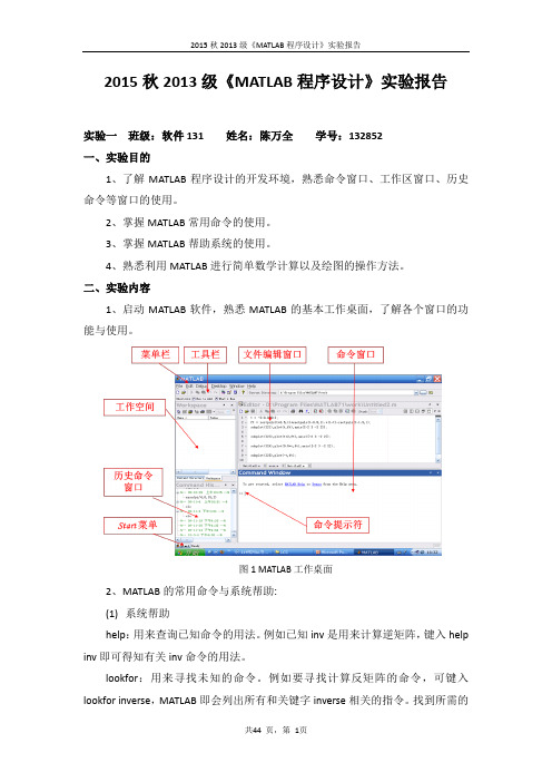
二、实验内容1、启动MATLAB软件,熟悉MATLAB的基本工作桌面,了解各个窗口的功能与使用。
图1 MATLAB工作桌面2、MATLAB的常用命令与系统帮助:(1)系统帮助help:用来查询已知命令的用法。
例如已知inv是用来计算逆矩阵,键入help inv即可得知有关inv命令的用法。
lookfor:用来寻找未知的命令。
例如要寻找计算反矩阵的命令,可键入lookfor inverse,MATLAB即会列出所有和关键字inverse相关的指令。
找到所需的命令後,即可用help进一步找出其用法。
(2)数据显示格式:常用命令:说明format short 显示小数点后4位(缺省值)format long 显示15位format bank 显示小数点后2位format + 显示+,-,0format short e 5位科学记数法format long e 15位科学记数法format rat 最接近的有理数显示(3)命令行编辑:键盘上的各种箭头和控制键提供了命令的重调、编辑功能。
具体用法如下:↑----重调前一行(可重复使用调用更早的)↓----重调后一行→----前移一字符←----后移一字符home----前移到行首end----移动到行末esc----清除一行del----清除当前字符backspace----清除前一字符(4)MATLAB工作区常用命令:who--------显示当前工作区中所有用户变量名whos--------显示当前工作区中所有用户变量名及大小、字节数和类型disp(x) -----显示变量X的内容clear -----清除工作区中用户定义的所有变量save文件名-----保存工作区中用户定义的所有变量到指定文件中load文件名-----载入指定文件中的数据三、源程序和实验结果1、在命令窗口执行命令完成以下运算,观察workspace 的变化,记录运算结果。
香农熵的matlab程序

香农熵的Matlab程序1. 引言香农熵(Shannon Entropy)是信息论中一个重要的概念,用于衡量一个随机变量的不确定性或者信息量。
在信息论和通信领域,香农熵被广泛应用于数据压缩、信号处理、密码学等方面。
本文将介绍如何使用Matlab编写程序来计算香农熵。
2. 算法原理香农熵的计算公式如下:其中,H表示香农熵,p(x)表示随机变量X取某个值x的概率。
根据该公式,我们需要计算每个可能取值的概率,并将其代入公式中求和,即可得到香农熵的值。
3. Matlab程序实现下面是一个简单的Matlab程序,用于计算给定随机变量的香农熵:function entropy = shannon_entropy(probabilities)entropy = 0;for i = 1:length(probabilities)if probabilities(i) ~= 0entropy = entropy - probabilities(i) * log2(probabilities(i));endendend以上程序定义了一个名为shannon_entropy的函数,该函数接受一个概率向量作为输入参数,并返回计算得到的香农熵。
程序的实现思路是遍历概率向量中的每个元素,如果该元素不为0,则将其代入香农熵的计算公式中进行计算,并累加到最终的结果中。
4. 使用示例为了演示程序的使用,我们将计算一个简单的示例。
假设有一个随机变量X,其可能取值为[1, 2, 3],对应的概率分别为[0.3, 0.5, 0.2]。
我们可以使用上述程序来计算该随机变量的香农熵。
probabilities = [0.3, 0.5, 0.2];entropy = shannon_entropy(probabilities);disp(['Entropy: ', num2str(entropy)]);运行上述代码,程序将输出以下结果:Entropy: 1.4854753这表明给定的随机变量X的香农熵为1.4854753。
matlab的程序流程控制实验总结

matlab的程序流程控制实验总结Matlab programming is a powerful tool that can be used to solve complex mathematical problems and analyze data. In order to fully utilize its capabilities, it is important to have a good understandingof program flow control in Matlab. Program flow control refers to the way in which the execution of a program is controlled in order to achieve the desired outcome. One of the most common ways to control the flow of a program in Matlab is through the use of loops. Loops allow you to iterate over a set of data or perform a series of operations multiple times. There are two main types of loops in Matlab: for loops and while loops. For loops are used when youknow the exact number of times you want to repeat a block of code, while loops are used when you want to repeat a block of code until a certain condition is met.在Matlab编程中,程序流程控制是一种强大的工具,可以用来解决复杂的数学问题和分析数据。
MATLAB程序设计
MATLAB程序设计MATLAB提供了一个完善的程序设计语言环境,使用户能够方便地编制复杂的程序,完成各种计算。
本节先介绍关系运算、逻辑运算,再介绍M-文件(即程序文件)的结构及MATLAB的程序控制流语句。
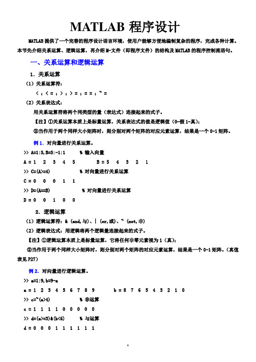
一、关系运算和逻辑运算1.关系运算(1)关系运算符:< ;< = ;> ;> = ;= = ;~ =(2)关系表达式:用关系运算符将两个同类型的量(表达式)连接起来的式子。
【注】①关系运算本质上是标量运算,关系表达式的值是逻辑值(0-假1-真);②当作用于两个同样大小矩阵时,则分别对两个矩阵的对应元素运算,结果是一个0-1矩阵。
例1.对向量进行关系运算。
>> A=1:5,B=5:-1:1 % 输入向量A = 1 2 3 4 5B = 5 4 3 2 1>> C=(A>=4) % 对向量进行关系运算C = 0 0 0 1 1>> D=(A==B) % 对向量进行关系运算D = 0 0 1 0 02.逻辑运算(1)逻辑运算符:& (and,与)、| (or,或)、~ (not,非)(2)逻辑表达式:用逻辑将两个逻辑量连接起来的式子。
【注】①逻辑运算本质上是标量运算,它将任何非零元素视为1(真);②当作用于两个同样大小矩阵时,则分别对两个矩阵的对应元素运算,结果是一个0-1矩阵。
(真值表见P27)例2.对向量进行逻辑运算。
>> a=1:9,b=9-aa = 1 2 3 4 5 6 7 8 9b = 8 7 6 5 4 3 2 1 0>> c=~(a>4) % 非运算c = 1 1 1 1 0 0 0 0 0>> d=(a>=3)&(b<6) % 与运算d = 0 0 0 1 1 1 1 1 13.逻辑函数any(x) 向量x 中有非零元返回1,否则返回0。
(向量函数) all(x) 向量x 中所有元素非零返回1,否则返回0。
MATLAB讲座5作业及答案(附程序)
C2=C2.^4
20
3、求 n! n1
Matlab 程序: clear all;clc;close all; n=20; sum=0; temp=1; for i=1:n
end end 2、已知 A=[2 13 23 5;7 4 12 9 ;10 17 4 5] ,B=eye (3),求 (1) A 中行的最大元素; (2) A 中列的最小元素; (3) 生成一个与 A 大小相等的单位阵; (4) C1=A’*B; (5) C2=A*B,C24 (6) C3=2A—3B Matlab 程序: clear all;clc;close all; A=[2 13 23 5;
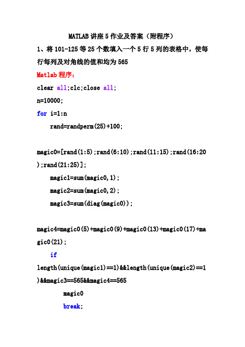
matlab讲座5作业及答案附程序1将101125等25个数填入一个5行5列的表格中使每行每列及对角线的值和均为5652已知a213235
MATLAB 讲座 5 作业及答案(附程序) 1、将 101-125 等 25 个数填入一个 5 行 5 列的表格中,使每 行每列及对角线的值和均为 565 Matlab 程序: clear all;clc;close all; n=10000; for i=1:n
temp=temp*i; sum=sum+temp; end sum
4、求以下数列极限:
(1) lim x0
x2 1 x sin x
c os x
1
1
(2Байду номын сангаас lim x 1-
1
,
lim
MATLAB实验及程序
实验一a=[1,2,3;4,5,6;7,8,9] b= repmat(a,2,2)B(24)=9实验二1、使用matlab命令统计randn(5)生成的矩阵里,有多少个元素小于0,将小于0元素个数存变量c中并将这些小于零元素存变量d中。
(实验报告要求:写出命令)a=randn(5)b=find(a<0);c=length(find(a<0))d=a(b)2、建立一个字符数组,内容如下所示:(实验报告要求:写出命令)A B C DE F G Ha b c da=['A B C D''E F G H''a b c d']3、已知有一个矩阵A(假如不知道其具体信息),请计算其元素个数(请先用实际矩阵来验证计算方法是否正确)。
(实验报告要求:写出正确计算方法的命令)A=randn(3,4)B=numel(A)4、已知有一个元胞数组B=[{ones(2,3,2)},{'Hello, Matlab'};{[4 5 6]},{1:100}],想获取字符串'Matlab',应输入什么命令?(实验报告要求:写出命令)f=B{1,2}(7:end)5、要从上题所建元胞数组B中获取列向量[4;5;6],可以有哪几种方法?(实验报告要求:写出命令及结果)方法1: i=B{2,1}(:)方法2: j=reshape(B{2,1},3,1)6、已知有两个学生的信息如下,请在matlab中创建结构对其进行存储,并算=['姓名''张三''李四']student.shuxue=[8778]student.yuwen=[7581 ]student.yingyu=[5560]实验三实验四:二维绘图(1)在同一个窗体(figure1)中画出正弦函数和余弦函数的图象。
要求如下:◆正弦图象用蓝色实线,时标用方格;◆余弦图象用黄色虚线,时标选向下三角形;◆为整个图像加中文标题;◆为x和y轴加轴标题;◆改x轴的单位为pi/2的倍数;◆增加图例;◆在图中合适的位置增加“正弦曲线”和“余弦曲线”两处文本信息。
matlab编写程序
mathematics Basic Matrix Operations>> a=[1 2 3 4 5]生成矩阵;>> b=a+2矩阵加上数字>> plot(b)画三点图>> grid on生成网格>> bar(b)生成条状图>> xlabel('sample#') 给X轴加标注>> ylabel('pound') 给Y轴加标注>> title('bar plot')加标题>> plot(b,'*')用*表示点>> axis([0 10 10 20 0 20])各个轴的范围>> A = [1 2 0; 2 5 -1; 4 10 -1]>> B=A'转置>> C=A*B矩阵相乘>> C=A.*B数组相乘>> X=inv(A)逆>> I=inv(A)*A单位矩阵>> eig(A)特征值>> svd(A) the singular value decomposition. 奇异值分解>> p = round(poly(A))生成特征多项式的系数>> roots(p) 特征多项式的根,即矩阵的特征值>> q = conv(p,p) 向量的卷积>> r = conv(p,q) 再向量的卷积>> plot(r)>> who 变量列表 >> whos 变量的详细列表>> sqrt(-1);>> sqrt(2) 开方Matrix Manipulation>> A = magic(3) 生成魔方矩阵graphics2-D PlotsLine Plot of a Chirp(线状图)>> doc plot 在帮助中查看plot更多的信息>> x=0:0.05:5;>> y=sin(x.^2);>> plot(x,y);>> plot(x,y,'o');>> xlabel('Time')>> ylabel('Amplitude')Bar Plot of a Bell Shaped Curve(条状图)>> x = -2.9:0.2:2.9;>> bar(x,exp(-x.*x));函数中包括了计算,plot直接完成Stairstep Plot of a Sine Wave(阶梯图)>> x=0:0.25:10;>> stairs(x,sin(x));Errorbar Plot>> x=-2:0.1:2;>> y=erf(x);>> y=erf(x);e = rand(size(x))/10>> errorbar(x,y,e);Polar Plot>> t=0:0.01:2*pi;>> polar(t,abs(sin(2*t).*cos(2*t))); abs绝对值Stem Plot>> x = 0:0.1:4;>> y = sin(x.^2).*exp(-x);>> stem(x,y)Scatter Plot>> load count.dat>> scatter(count(:,1),count(:,2),'r*')>> xlabel('Number of Cars on Street A');>> ylabel('Number of Cars on Street B');更多plot的类型可以在命令行输入doc praph2d查看3-D PlotsMesh Plot of Peaks>> z=peaks(25);peaks is a function of two variables, obtained by translating and scaling Gaussian distributions, which is useful for demonstrating mesh, surf, pcolor, contour, and so on.>> mesh(z);>> meshc(z);带有轮廓线>> colormap(hsv);对mesh的图象使用不同的色彩,如gray, hot, bone. EtcSurface Plot of Peaks>> z=peaks(25);>> surf(z); 3-D shaded surface plot>> surfc(z);带有轮廓线>> colormap jet;同>> colormap(jet); 对mesh的图象使用不同的色彩Surface Plot (with Shading) of Peaks>> z=peaks(25);>> surfl(z); Surface plot with colormap-based lighting>> shading interp; Set color shading properties>> colormap(pink);Contour Plot of Peaks>> z=peaks(25);>> contour(z,16) 轮廓线>> colormap(hsv)Quiver (Quiver or velocity plot)>> x = -2:.2:2;>> y = -1:.2:1;>> [xx,yy] = meshgrid(x,y);>> zz = xx.*exp(-xx.^2-yy.^2);>> [px,py] = gradient(zz,.2,.2);>> quiver(x,y,px,py,2);Slice(Volumetric slice plot)>> [x,y,z] = meshgrid(-2:.2:2,-2:.25:2,-2:.16:2);>> v = x.*exp(-x.^2-y.^2-z.^2);>> xslice = [-1.2,.8,2];>> yslice = 2;>> zslice = [-2,0];>> [x,y,z] = meshgrid(-2:.2:2,-2:.25:2,-2:.16:2); >> slice(x,y,z,v,xslice,yslice,zslice)>> colormap hsvProgramming Manipulating Multidimensional Arrays Creating Multi-Dimensional ArraysThe CAT function is a useful tool for building multidimensional arrays. B = cat(DIM,A1,A2,...) builds a multidimensional array by concatenating A1, A2 ... along the dimension DIM.Calls to CAT can be nested.>> B = cat( 3, [2 8; 0 5], [1 3; 7 9], [2 3; 4 6]); B(:,:,1) =2 80 5B(:,:,2) =1 37 9B(:,:,3) =2 34 6>> A = cat(3,[9 2; 6 5], [7 1; 8 4]);>> B = cat(3,[3 5; 0 1], [5 6; 2 1]);>> C = cat(4,A,B,cat(3,[1 2; 3 4], [4 3; 2 1])); C(:,:,1,1) =9 26 5C(:,:,2,1) =7 18 4C(:,:,1,2) =3 50 1C(:,:,2,2) =5 62 1C(:,:,1,3) =1 23 4C(:,:,2,3) =4 32 1>> A = cat(2,[9 2; 6 5], [7 1; 8 4]);>> B = cat(2,[3 5; 0 1], [5 6; 2 1]);>> C = cat(4,A,B,cat(2,[1 2; 3 4], [4 3; 2 1]))C(:,:,1,1) =9 2 7 16 5 8 4C(:,:,1,2) =3 5 5 60 1 2 1C(:,:,1,3) =1 2 4 33 4 2 1>> C = cat(2,A,B,cat(2,[1 2; 3 4], [4 3; 2 1]))C =9 2 7 1 3 5 5 6 1 2 4 3;6 5 8 4 0 1 2 1 3 4 2 1>> C = cat(1,A,B,cat(2,[1 2; 3 4], [4 3; 2 1]))C =9 2 7 1 6 5 8 4 3 5 5 60 1 2 11 2 4 3 3 4 2 1 Finding the Dimensions >>SzA = size(A)>>DimsA = ndims(A)>>SzC = size(C)>>DimsC = ndims(C) Accessing Elements>> K = C(:,:,1,[1 3])K(:,:,1,1) =9 26 5K(:,:,1,2) =1 23 4Manipulating Multi-Dimensional Arrays>> A = rand(3,3,2);>> B = permute(A, [2 1 3]);>> C = permute(A, [3 2 1]);Selecting 2D Matrices From Multi-Dimensional Arrays >> A = cat( 3, [1 2 3; 9 8 7; 4 6 5], [0 3 2; 8 8 4;5 3 5], ...[6 4 7; 6 8 5; 5 4 3]);>>% The EIG function is applied to each of the horizontal 'slices' of A.for i = 1:3eig(squeeze(A(i,:,:)))end>> x1 = -2*pi:pi/10:0;>> x2 = 2*pi:pi/10:4*pi;>> x3 = 0:pi/10:2*pi;>> [x1,x2,x3] = ndgrid(x1,x2,x3);>> z = x1 + exp(cos(2*x2.^2)) + sin(x3.^3);>> slice(z,[5 10 15], 10, [5 12]);>> axis tight;Structures% Draw a visualization of a structure.>> strucdem_helper(1)>> = 'John Doe';>> patient.billing = 127.00;>> patient.test = [79 75 73; 180 178 177.5; 172 170 169]; >> patientpatient =name: 'John Doe'billing: 127test: [3x3 double]>> patient(2).name = 'Ann Lane';>> patient(2).billing = 28.50;>> patient(2).test = [68 70 68; 118 118 119; 172 170 169];% Update the visualization.>> strucdem_helper(2);>> fnames1 = fieldnames(patient)>> patient2 = rmfield(patient,'test');>> fnames2 = fieldnames(patient2)fnames1 ='name''billing''test'fnames2 ='name''billing'>> A = struct( 'data', {[3 4 7; 8 0 1], [9 3 2; 7 6 5]}, ... 'nest', {...struct( 'testnum', 'Test 1', ... 'xdata', [4 2 8], 'ydata', [7 1 6]), ... struct( 'testnum', 'Test 2', ... 'xdata', [3 4 2], 'ydata', [5 0 9])}) % Update the visualization.>> strucdem_helper(3)聚类分析K(C)均值算法:x=[-7.82 -4.58 -3.97;-6.68 3.16 2.17;4.36 -2.19 2.09;6.72 0.88 2.80;...] -8.64 3.06 3.5;-6.87 0.57 -5.45;4.47 -2.62 5.76;6.73 -2.01 4.18;... -7.71 2.34 -6.33;-6.91 -0.49 -5.68;6.18 2.81 5.82;6.72 -0.93 -4.04;... -6.25 -0.26 0.56;-6.94 -1.22 1.13;8.09 0.20 2.25;6.81 0.17 -4.15;... -5.19 4.24 4.04;-6.38 -1.74 1.43;4.08 1.3 5.33;6.27 0.93 -2.78];[idx,ctrs]=kmeans(x,3)如何编写求K-均值聚类算法的Matlab程序在聚类分析中,K-均值聚类算法(k-means algorithm)是无监督分类中的一种基本方法,其也称为C-均值算法,其基本思想是:通过迭代的方法,逐次更新各聚类中心的值,直至得到最好的聚类结果。
matlab教程(完整版)
01 MATLABChapterMATLAB简介MATLAB是一种高级编程语言和环境,主要用于数值计算、数据分析、信号处理、图像处理等多种应用领域。
MATLAB具有简单易学、高效灵活、可视化强等特点,被广泛应用于科研、工程、教育等领域。
MATLAB提供了丰富的函数库和工具箱,方便用户进行各种复杂的数学计算和数据分析。
MATLAB安装与启动MATLAB界面介绍工作空间用于显示当前定义的所有变量及其值。
命令历史记录了用户输入过的命令及其输出结果。
基本运算与数据类型02矩阵运算与数组操作Chapter01020304使用`[]`或`zeros`、`ones`等函数创建矩阵创建矩阵使用`size`函数获取矩阵大小矩阵大小通过下标访问矩阵元素,如`A(i,j)`矩阵元素访问使用`disp`或`fprintf`函数显示矩阵信息矩阵信息矩阵创建与基本操作对应元素相加,如`C = A+ B`加法运算矩阵运算对应元素相减,如`C = A-B`减法运算数与矩阵相乘,如`B = k *A`数乘运算使用单引号`'`进行转置,如`B = A'`转置运算满足乘法条件的矩阵相乘,如`C = A * B`矩阵乘法使用`inv`函数求逆矩阵,如`B = inv(A)`逆矩阵数组创建数组大小数组元素访问数组操作数组操作01020304线性方程组求解数据处理与分析特征值与特征向量图像处理矩阵与数组应用实例03数值计算与数据分析Chapter数值计算基础MATLAB基本运算数值类型与精度变量与表达式函数与脚本数据分析方法数据导入与预处理学习如何导入各种格式的数据(如Excel、CSV、TXT等),并进行数据清洗、转换等预处理操作。
数据统计描述掌握MATLAB中数据统计描述的方法,如计算均值、中位数、标准差等统计量,以及绘制直方图、箱线图等统计图表。
数据相关性分析学习如何在MATLAB中进行数据相关性分析,如计算相关系数、绘制散点图等。
matlab仿真程序
4.搜集整理小波分析的matlab程序4.1小波滤波器构造和消噪程序重构% mallet_wavelet.m% 此函数用于研究Mallet算法及滤波器设计% 此函数仅用于消噪a=pi/8; %角度赋初值b=pi/8;%低通重构FIR滤波器h0(n)冲激响应赋值h0=cos(a)*cos(b);h1=sin(a)*cos(b);h2=-sin(a)*sin(b);h3=cos(a)*sin(b);low_construct=[h0,h1,h2,h3];L_fre=4; %滤波器长度low_decompose=low_construct(end:-1:1); %确定h0(-n),低通分解滤波器for i_high=1:L_fre; %确定h1(n)=(-1)^n,高通重建滤波器if(mod(i_high,2)==0);coefficient=-1;elsecoefficient=1;endhigh_construct(1,i_high)=low_decompose(1,i_high)*coefficient;endhigh_decompose=high_construct(end:-1:1); %高通分解滤波器h1(-n) L_signal=100; %信号长度n=1:L_signal; %信号赋值f=10;t=0.001;y=10*cos(2*pi*50*n*t).*exp(-20*n*t);figure(1);plot(y);title('原信号');check1=sum(high_decompose); %h0(n)性质校验check2=sum(low_decompose);check3=norm(high_decompose);check4=norm(low_decompose);l_fre=conv(y,low_decompose); %卷积l_fre_down=dyaddown(l_fre); %抽取,得低频细节h_fre=conv(y,high_decompose);h_fre_down=dyaddown(h_fre); %信号高频细节figure(2);subplot(2,1,1)plot(l_fre_down);title('小波分解的低频系数');subplot(2,1,2);plot(h_fre_down);title('小波分解的高频系数');l_fre_pull=dyadup(l_fre_down); %0差值h_fre_pull=dyadup(h_fre_down);l_fre_denoise=conv(low_construct,l_fre_pull);h_fre_denoise=conv(high_construct,h_fre_pull);l_fre_keep=wkeep(l_fre_denoise,L_signal); %取结果的中心部分,消除卷积影响h_fre_keep=wkeep(h_fre_denoise,L_signal);sig_denoise=l_fre_keep+h_fre_keep; %信号重构compare=sig_denoise-y; %与原信号比较figure(3);subplot(3,1,1)plot(y);ylabel('y'); %原信号subplot(3,1,2);plot(sig_denoise);ylabel('sig\_denoise'); %重构信号subplot(3,1,3);plot(compare);ylabel('compare'); %原信号与消噪后信号的比较消噪、% 此函数用于研究Mallet算法及滤波器设计% 此函数用于消噪处理%角度赋值%此处赋值使滤波器系数恰为db9%分解的高频系数采用db9较好,即它的消失矩较大%分解的有用信号小波高频系数基本趋于零%对于噪声信号高频分解系数很大,便于阈值消噪处理[l,h]=wfilters('db10','d');low_construct=l;L_fre=20; %滤波器长度low_decompose=low_construct(end:-1:1); %确定h0(-n),低通分解滤波器for i_high=1:L_fre; %确定h1(n)=(-1)^n,高通重建滤波器if(mod(i_high,2)==0);coefficient=-1;elsecoefficient=1;endhigh_construct(1,i_high)=low_decompose(1,i_high)*coefficient;endhigh_decompose=high_construct(end:-1:1); %高通分解滤波器h1(-n)L_signal=100; %信号长度n=1:L_signal; %原始信号赋值f=10;t=0.001;y=10*cos(2*pi*50*n*t).*exp(-30*n*t);zero1=zeros(1,60); %信号加噪声信号产生zero2=zeros(1,30);noise=[zero1,3*(randn(1,10)-0.5),zero2];y_noise=y+noise;figure(1);subplot(2,1,1);plot(y);title('原信号');subplot(2,1,2);plot(y_noise);title('受噪声污染的信号');check1=sum(high_decompose); %h0(n),性质校验check2=sum(low_decompose);check3=norm(high_decompose);check4=norm(low_decompose);l_fre=conv(y_noise,low_decompose); %卷积l_fre_down=dyaddown(l_fre); %抽取,得低频细节h_fre=conv(y_noise,high_decompose);h_fre_down=dyaddown(h_fre); %信号高频细节subplot(2,1,1)plot(l_fre_down);title('小波分解的低频系数');subplot(2,1,2);plot(h_fre_down);title('小波分解的高频系数');% 消噪处理for i_decrease=31:44;if abs(h_fre_down(1,i_decrease))>=0.000001h_fre_down(1,i_decrease)=(10^-7);endendl_fre_pull=dyadup(l_fre_down); %0差值h_fre_pull=dyadup(h_fre_down);l_fre_denoise=conv(low_construct,l_fre_pull);h_fre_denoise=conv(high_construct,h_fre_pull);l_fre_keep=wkeep(l_fre_denoise,L_signal); %取结果的中心部分,消除卷积影响h_fre_keep=wkeep(h_fre_denoise,L_signal);sig_denoise=l_fre_keep+h_fre_keep; %消噪后信号重构%平滑处理for j=1:2sig_denoise(i)=sig_denoise(i-2)+sig_denoise(i+2)/2;end;end;compare=sig_denoise-y; %与原信号比较figure(3);subplot(3,1,1)plot(y);ylabel('y'); %原信号subplot(3,1,2);plot(sig_denoise);ylabel('sig\_denoise'); %消噪后信号subplot(3,1,3);plot(compare);ylabel('compare'); %原信号与消噪后信号的比较4.2小波谱分析mallat算法经典程序clc;clear;%% 1.正弦波定义f1=50; % 频率1f2=100; % 频率2fs=2*(f1+f2); % 采样频率Ts=1/fs; % 采样间隔N=120; % 采样点数n=1:N;y=sin(2*pi*f1*n*Ts)+sin(2*pi*f2*n*Ts); % 正弦波混合figure(1)plot(y);title('两个正弦信号')figure(2)stem(abs(fft(y)));title('两信号频谱')%% 2.小波滤波器谱分析h=wfilters('db30','l'); % 低通g=wfilters('db30','h'); % 高通h=[h,zeros(1,N-length(h))]; % 补零(圆周卷积,且增大分辨率变于观察)g=[g,zeros(1,N-length(g))]; % 补零(圆周卷积,且增大分辨率变于观察)figure(3);stem(abs(fft(h)));title('低通滤波器图')figure(4);stem(abs(fft(g)));title('高通滤波器图')%% 3.MALLET分解算法(圆周卷积的快速傅里叶变换实现)sig1=ifft(fft(y).*fft(h)); % 低通(低频分量)sig2=ifft(fft(y).*fft(g)); % 高通(高频分量)figure(5); % 信号图subplot(2,1,1)plot(real(sig1));title('分解信号1')subplot(2,1,2)plot(real(sig2));title('分解信号2')figure(6); % 频谱图subplot(2,1,1)stem(abs(fft(sig1)));title('分解信号1频谱')subplot(2,1,2)stem(abs(fft(sig2)));title('分解信号2频谱')%% 4.MALLET重构算法sig1=dyaddown(sig1); % 2抽取sig2=dyaddown(sig2); % 2抽取sig1=dyadup(sig1); % 2插值sig2=dyadup(sig2); % 2插值sig1=sig1(1,[1:N]); % 去掉最后一个零sig2=sig2(1,[1:N]); % 去掉最后一个零hr=h(end:-1:1); % 重构低通gr=g(end:-1:1); % 重构高通hr=circshift(hr',1)'; % 位置调整圆周右移一位gr=circshift(gr',1)'; % 位置调整圆周右移一位sig1=ifft(fft(hr).*fft(sig1)); % 低频sig2=ifft(fft(gr).*fft(sig2)); % 高频sig=sig1+sig2; % 源信号%% 5.比较figure(7);subplot(2,1,1)plot(real(sig1));title('重构低频信号');subplot(2,1,2)plot(real(sig2));title('重构高频信号');figure(8);subplot(2,1,1)stem(abs(fft(sig1)));title('重构低频信号频谱');subplot(2,1,2)stem(abs(fft(sig2)));title('重构高频信号频谱');figure(9)plot(real(sig),'r','linewidth',2);hold on;plot(y);legend('重构信号','原始信号')title('重构信号与原始信号比较')小波包变换分析信号的MATLAB程序%t=0.001:0.001:1;t=1:1000;s1=sin(2*pi*50*t*0.001)+sin(2*pi*120*t*0.001)+rand(1,length(t));for t=1:500;s2(t)=sin(2*pi*50*t*0.001)+sin(2*pi*120*t*0.001)+rand(1,length(t)); endfor t=501:1000;s2(t)=sin(2*pi*200*t*0.001)+sin(2*pi*120*t*0.001)+rand(1,length(t)); endsubplot(9,2,1)plot(s1)title('原始信号')ylabel('S1')subplot(9,2,2)plot(s2)title('故障信号')ylabel('S2')wpt=wpdec(s1,3,'db1','shannon');%plot(wpt);s130=wprcoef(wpt,[3,0]);s131=wprcoef(wpt,[3,1]);s132=wprcoef(wpt,[3,2]);s133=wprcoef(wpt,[3,3]);s134=wprcoef(wpt,[3,4]);s135=wprcoef(wpt,[3,5]);s136=wprcoef(wpt,[3,6]);s137=wprcoef(wpt,[3,7]);s10=norm(s130);s11=norm(s131);s12=norm(s132);s13=norm(s133);s14=norm(s134);s15=norm(s135);s16=norm(s136);s17=norm(s137);st10=std(s130);st11=std(s131);st12=std(s132);st13=std(s133);st14=std(s134);st15=std(s135);st16=std(s136);st17=std(s137);disp('正常信号的特征向量');snorm1=[s10,s11,s12,s13,s14,s15,s16,s17] std1=[st10,st11,st12,st13,st14,st15,st16,st17]subplot(9,2,3);plot(s130);ylabel('S130');subplot(9,2,5);plot(s131);ylabel('S131');subplot(9,2,7);plot(s132);ylabel('S132');subplot(9,2,9);plot(s133);ylabel('S133');subplot(9,2,11);plot(s134);ylabel('S134');subplot(9,2,13);plot(s135);ylabel('S135');subplot(9,2,15);plot(s136);ylabel('S136');subplot(9,2,17);plot(s137);ylabel('S137');wpt=wpdec(s2,3,'db1','shannon');%plot(wpt);s230=wprcoef(wpt,[3,0]);s231=wprcoef(wpt,[3,1]);s232=wprcoef(wpt,[3,2]);s233=wprcoef(wpt,[3,3]);s234=wprcoef(wpt,[3,4]);s235=wprcoef(wpt,[3,5]);s236=wprcoef(wpt,[3,6]);s237=wprcoef(wpt,[3,7]);s20=norm(s230);s21=norm(s231);s22=norm(s232);s23=norm(s233);s24=norm(s234);s25=norm(s235);s26=norm(s236);s27=norm(s237);st20=std(s230);st21=std(s231);st22=std(s232);st23=std(s233);st24=std(s234);st25=std(s235);st26=std(s236);st27=std(s237);disp('故障信号的特征向量');snorm2=[s20,s21,s22,s23,s24,s25,s26,s27] std2=[st20,st21,st22,st23,st24,st25,st26,st27]subplot(9,2,4);plot(s230);ylabel('S230');subplot(9,2,6);plot(s231); ylabel('S231');subplot(9,2,8);plot(s232); ylabel('S232');subplot(9,2,10);plot(s233); ylabel('S233');subplot(9,2,12);plot(s234); ylabel('S234');subplot(9,2,14);plot(s235); ylabel('S235');subplot(9,2,16);plot(s236); ylabel('S236');subplot(9,2,18);plot(s237); ylabel('S237');%fftfigurey1=fft(s1,1024);py1=y1.*conj(y1)/1024;y2=fft(s2,1024);py2=y2.*conj(y2)/1024;y130=fft(s130,1024);py130=y130.*conj(y130)/1024; y131=fft(s131,1024);py131=y131.*conj(y131)/1024; y132=fft(s132,1024);py132=y132.*conj(y132)/1024; y133=fft(s133,1024);py133=y133.*conj(y133)/1024; y134=fft(s134,1024);py134=y134.*conj(y134)/1024; y135=fft(s135,1024);py135=y135.*conj(y135)/1024; y136=fft(s136,1024);py136=y136.*conj(y136)/1024; y137=fft(s137,1024);py137=y137.*conj(y137)/1024;y230=fft(s230,1024);py230=y230.*conj(y230)/1024; y231=fft(s231,1024);py231=y231.*conj(y231)/1024; y232=fft(s232,1024);py232=y232.*conj(y232)/1024; y233=fft(s233,1024);py233=y233.*conj(y233)/1024; y234=fft(s234,1024);py234=y234.*conj(y234)/1024; y235=fft(s235,1024);py235=y235.*conj(y235)/1024; y236=fft(s236,1024);py236=y236.*conj(y236)/1024; y237=fft(s237,1024);py237=y237.*conj(y237)/1024;f=1000*(0:511)/1024; subplot(1,2,1);plot(f,py1(1:512));ylabel('P1');title('原始信号的功率谱') subplot(1,2,2);plot(f,py2(1:512));ylabel('P2');title('故障信号的功率谱') figuresubplot(4,2,1);plot(f,py130(1:512));ylabel('P130');title('S130的功率谱') subplot(4,2,2);plot(f,py131(1:512));ylabel('P131');title('S131的功率谱') subplot(4,2,3);plot(f,py132(1:512));ylabel('P132');subplot(4,2,4);plot(f,py133(1:512));ylabel('P133');subplot(4,2,5);plot(f,py134(1:512));ylabel('P134');subplot(4,2,6);plot(f,py135(1:512));ylabel('P135');subplot(4,2,7);plot(f,py136(1:512));ylabel('P136');subplot(4,2,8);plot(f,py137(1:512));ylabel('P137');figuresubplot(4,2,1);plot(f,py230(1:512));ylabel('P230');title('S230的功率谱')subplot(4,2,2);plot(f,py231(1:512));ylabel('P231');title('S231的功率谱')subplot(4,2,3);plot(f,py232(1:512));ylabel('P232');subplot(4,2,4);plot(f,py233(1:512));ylabel('P233');subplot(4,2,5);plot(f,py234(1:512));ylabel('P234');subplot(4,2,6);plot(f,py235(1:512));ylabel('P235');subplot(4,2,7);plot(f,py236(1:512));ylabel('P236');subplot(4,2,8);plot(f,py237(1:512));ylabel('P237');figure%plottree(wpt)4.3利用小波变换实现对电能质量检测的算法实现N=10000;s=zeros(1,N);for n=1:Nif n<0.4*N||n>0.8*Ns(n)=31.1*sin(2*pi*50/10000*n);elses(n)=22.5*sin(2*pi*50/10000*n);endendl=length(s);[c,l]=wavedec(s,6,'db5'); %用db5小波分解信号到第六层subplot(8,1,1);plot(s);title('用db5小波分解六层:s=a6+d6+d5+d4+d3+d2+d1'); Ylabel('s');%对分解结构【c,l】中第六层低频部分进行重构a6=wrcoef('a',c,l,'db5',6);subplot(8,1,2);plot(a6);Ylabel('a6');%对分解结构【c,l】中各层高频部分进行重构for i=1:6decmp=wrcoef('d',c,l,'db5',7-i);subplot(8,1,i+2);plot(decmp);Ylabel(['d',num2str(7-i)]);end%-----------------------------------------------------------rec=zeros(1,300);rect=zeros(1,300);ke=1;u=0;d1=wrcoef('d',c,l,'db5',1);figure(2);plot(d1);si=0;N1=0;N0=0;sce=0;for n=20:N-30rect(ke)=s(n);ke=ke+1;if(ke>=301)if(si==2)rec=rect;u=2;end;si=0;ke=1;end;if(d1(n)>0.01) % the condition of abnormal append.N1=n;if(N0==0)N0=n;si=si+1;end;if(N1>N0+30)Nlen=N1-N0;Tab=Nlen/10000;end;end;if(si==1)for k=N0:N0+99 %testing of 1/4 period signals to sce=sce+s(k)*s(k)/10000;end;re=sqrt(sce*200) %re indicate the pike value of .sce=0;si=si+1;end;end;NlenN0n=1:300;figure(3)plot(n,rec);4.4基于小波变换的图象去噪Normalshrink算法function [T_img,Sub_T]=threshold_2_N(img,levels)% reference :image denoising using wavelet thresholding[xx,yy]=size(img);HH=img((xx/2+1):xx,(yy/2+1):yy);delt_2=(std(HH(:)))^2;%(median(abs(HH(:)))/0.6745)^2;%T_img=img;for i=1:levelstemp_x=xx/2^i;temp_y=yy/2^i;% belt=1.0*(log(temp_x/(2*levels)))^0.5;belt=1.0*(log(temp_x/(2*levels)))^0.5; %2.5 0.8%HLHL=img(1:temp_x,(temp_y+1):2*temp_y);delt_y=std(HL(:));T_1=belt*delt_2/delt_y;%%%%%%%%%%%%%%%%%%%%%%%%%%%%%%%%%%%%%%%%%%%%% %%%T_HL=sign(HL).*max(0,abs(HL)-T_1);%%%%%%%%%%%%%%%%%%%%%%%%%%%%%%%%%%%%%%%%%%%%% %%T_img(1:temp_x,(temp_y+1):2*temp_y)=T_HL;Sub_T(3*(i-1)+1)=T_1;%LHLH=img((temp_x+1):2*temp_x,1:temp_y);delt_y=std(LH(:));T_2=belt*delt_2/delt_y;%%%%%%%%%%%%%%%%%%%%%%%%%%%%%%%%%%%%%%%%%%%%% %%T_LH=sign(LH).*max(0,abs(LH)-T_2);%%%%%%%%%%%%%%%%%%%%%%%%%%%%%%%%%%%%%%%%%%%%% %%%%T_img((temp_x+1):2*temp_x,1:temp_y)=T_LH;Sub_T(3*(i-1)+2)=T_2;%HHHH=img((temp_x+1):2*temp_x,(temp_y+1):2*temp_y);delt_y=std(HH(:));T_3=belt*delt_2/delt_y;%%%%%%%%%%%%%%%%%%%%%%%%%%%%%%%%%%%%%%%%%%%%% %%%%%%%%%T_HH=sign(HH).*max(0,abs(HH)-T_3);%%%%%%%%%%%%%%%%%%%%%%%%%%%%%%%%%%%%%%%%%%%%% %%%%%%%%T_img((temp_x+1):2*temp_x,(temp_y+1):2*temp_y)=T_HH;Sub_T(3*(i-1)+3)=T_3;end4.5小波去噪matlab程序****************************************** clearclc%在噪声环境下语音信号的增强%语音信号为读入的声音文件%噪声为正态随机噪声sound=wavread('c12345.wav');count1=length(sound);noise=0.05*randn(1,count1);for i=1:count1signal(i)=sound(i);endfor i=1:count1y(i)=signal(i)+noise(i);end%在小波基'db3'下进行一维离散小波变换[coefs1,coefs2]=dwt(y,'db3'); %[低频高频] count2=length(coefs1);count3=length(coefs2);energy1=sum((abs(coefs1)).^2); energy2=sum((abs(coefs2)).^2); energy3=energy1+energy2;for i=1:count2recoefs1(i)=coefs1(i)/energy3;endfor i=1:count3recoefs2(i)=coefs2(i)/energy3;end%低频系数进行语音信号清浊音的判别zhen=160;count4=fix(count2/zhen);for i=1:count4n=160*(i-1)+1:160+160*(i-1);s=sound(n);w=hamming(160);sw=s.*w;a=aryule(sw,10);sw=filter(a,1,sw);sw=sw/sum(sw);r=xcorr(sw,'biased');corr=max(r);%为清音(unvoice)时,输出为1;为浊音(voice)时,输出为0 if corr>=0.8output1(i)=0;elseif corr<=0.1output1(i)=1;endendfor i=1:count4n=160*(i-1)+1:160+160*(i-1);if output1(i)==1switch abs(recoefs1(i))case abs(recoefs1(i))<=0.002recoefs1(i)=0;case abs(recoefs1(i))>0.002 & abs(recoefs1(i))<=0.003recoefs1(i)=sgn(recoefs1(i))*(0.003*abs(recoefs1(i))-0.000003)/0.002; otherwise recoefs1(i)=recoefs1(i);endelseif output1(i)==0recoefs1(i)=recoefs1(i);endend%对高频系数进行语音信号清浊音的判别count5=fix(count3/zhen);for i=1:count5n=160*(i-1)+1:160+160*(i-1);s=sound(n);w=hamming(160);sw=s.*w;a=aryule(sw,10);sw=filter(a,1,sw);sw=sw/sum(sw);r=xcorr(sw,'biased');corr=max(r);%为清音(unvoice)时,输出为1;为浊音(voice)时,输出为0 if corr>=0.8output2(i)=0;elseif corr<=0.1output2(i)=1;endendfor i=1:count5n=160*(i-1)+1:160+160*(i-1);if output2(i)==1switch abs(recoefs2(i))case abs(recoefs2(i))<=0.002recoefs2(i)=0;case abs(recoefs2(i))>0.002 & abs(recoefs2(i))<=0.003recoefs2(i)=sgn(recoefs2(i))*(0.003*abs(recoefs2(i))-0.000003)/0.002; otherwise recoefs2(i)=recoefs2(i);endelseif output2(i)==0recoefs2(i)=recoefs2(i);endend%在小波基'db3'下进行一维离散小波反变换output3=idwt(recoefs1, recoefs2,'db3');%对输出信号抽样点值进行归一化处理maxdata=max(output3);output4=output3/maxdata;%读出带噪语音信号,存为'101.wav'wavwrite(y,5500,16,'c101');%读出处理后语音信号,存为'102.wav'wavwrite(output4,5500,16,'c102');4.6 神经网络小波Matlab实现%%%%%%%%%%%%%%%%%%%%%%%%%%%%%%%%%%%%%%%%%%%%%%% %%clear allload dataM1=20;epo=15;A=4;B=18;B2=B/2+1N=500;M=(A+1)*(B+1);for a0=1:A+1;for b0=1:B+1;i=(B+1)*(a0-1)+b0;b_init(i)=((b0-B2)/10)/(2^(-A)); a_init(i)=1/(2^(-A));c_init(i)=(20-A)/2;endendw0=ones(1,M);for i=1:Nfor j=1:Mt=x(i);t= a_init(j)*t-b_init(j);%P0(i,j)= (cos(1.75*t)*exp(-t*t/2))/2^c_init(j);P0(i,j)= ((1-t*t)*exp(-t*t/2))/2^c_init(j);endend%calculation of output of networkfor i=1:Nu=0;for j=1:Mu=u+w0(j)*P0(i,j);%w0?aè¨?μendy0(i)= u;% y(p)= u=??W(j)*phi(p,j)= ??W(j)* |μj(t)end %%%%%%%%%%%%%%%%%%%%%%%%%%%%%%%%%%%%%%%%%%%%%%% %%for k=1:MW(:,k)=P0(:,k);endfor k=2:Mu=0;for i=1:k-1aik(i)=(P0(:,k)'*W(:,i))/(W(:,i)'*W(:,i));u=u+aik(i) *W(:,i);endW(:,k)=P0(:,k)-u;end%%%%%%%%%%%%%%%%%%%%%%%%%%%%%%%%%%%%%%%%%%%%%%% %%%%for i=1:Mg(i)= (W(:,i)'*d')/( W(:,i)'* W(:,i));end %%%%%%%%%%%%%%%%%%%%%%%%%%%%%%%%%%%%%%%%%%%%%%% %%u=0;for i=1:Mu=u+g(i)*(W(:,i)'*W(:,i));endDD=u;for i=1:MErro(i)=(g(i)^2)*(W(:,i)'*W(:,i))/DD;end %%%%%%%%%%%%%%%%%%%%%%%%%%%%%%%%%%%%%%%%%%%%%%% %%k=1;while(k<=M1)u=1;for i=2:Mif abs(Erro(u))<abs(Erro(i));u=ielse u=uendendI(k)=u;Erro(u)=0k=k+1;end%%%%%%%%%%%%%%%%%%%%%%%%%%%%%%%%%%%%%%%%%%%%%%% %%for k=1:M1u=I(k);a(k)=a_init(u);b(k)=b_init(u);c(k)=c_init(u);w1(k)=w0(u);end %%%%%%%%%%%%%%%%%%%%%%%%%%%%%%%%%%%%%%%%%%%%%%% %%epoch=1;error=0.1;err=0.0001;lin=0.5;while (error>=err & epoch<=epo)for i=1:Nfor j=1:M1t=x(i);t= a(j)*t-b(j);%P1(i,j)= (cos(1.75*t)*exp(-t*t/2))/2^c(j);P1(i,j)= ((1-t*t)*exp(-t*t/2))/2^c(j);endend%calculation of output of networkfor i=1:Nu=0;for j=1:M1u=u+w1(j)*P1(i,j);endy1(i)= u;end %%%%%%%%%%%%%%%%%%%%%%%%%%%%%%%%%%%%%%%%%%%%%%% %%u=0;for i=1:Nu=u+(d(i)-y1(i))^2;endu=u/2;%u=1/2??(d-p)^2 %%%%%%%%%%%%%%%%%%%%%%%%%%%%%%%%%%%%%%%%%%%%%%% %%if u>errorlin=lin*0.8;elselin=lin*1.2;enderror=u; %error=u=1/2??(d-p)^2 %%%%%%%%%%%%%%%%%%%%%%%%%%%%%%%%%%%%%%%%%%%%%%% %%for j=1:M1u=0;for i=1:Nu=u+(d(i)-y1(i))*P1(i,j);endEW(j)=-u;endif epoch==1SW=-EW;w1_=w1;elseSW=-EW+((EW*EW')*SW_)/(EW_*EW_');endEW_=EW;SW_=SW;w1=w1_+SW*lin;w1_=w1;%number of epoch increase by 1epoch=epoch+1;end %%%%%%%%%%%%%%%%%%%%%%%%%%%%%%%%%%%%%%%%%%%%%%% %%subplot(2,1,1);plot(x,d);subplot(2,1,2);plot(x,y1);Matlab程序如下:function sd=liu_denoise(mix_signal)%此函数用于去除白躁信号&周期性干扰信号%输入参数mix_signal为采集到的信号波形p=0.6745;w_dept=9;w_name='db6';coef=cell(1,w_dept);thr=zeros(1,w_dept+1);[c,l]=wavedec(mix_signal,w_dept,w_name); %对混合信号S进行db6的9尺度一维分解coef(1)={appcoef(c,l,w_name,w_dept)};%计算尺度为9的一维分解低频系数cs=[cs,coef_soft{j}];thr(1)=median(abs(coef{1}))/p*sqrt(2*log(length(coef{1})));%计算1尺度上的阈值coef_soft(1)={wthresh(coef{1},'h',thr(1))};%对小波系数进行阈值为thr(1)的硬阈值处理cs=[coef_soft{1}];for j=2:w_dept+1coef(j)={detcoef(c,l,w_dept-j+2)};%计算尺度为9到2的各尺度高频小波系数coef1(j)={detcoef(c,l,w_dept-j+2)};thr(j)=median(abs(coef{j}))/p*sqrt(2*log(length(coef{j})));%计算9到2各尺度上的阈值coef_soft(j)={wthresh(coef{j},'h',thr(j))};%对小波系数进行阈值为thr(j)的硬阈值处理cs=[cs,coef_soft{j}];endsd=waverec(cs,l,w_name); %根据小波系数[cs,l]对信号进行重构4.2.2仿真分析为了验证去噪的有效性,先仿真产生一个局放脉冲然后叠加0.1倍白噪声和周期干扰,利用前面的程序去造,结果如图1,从图上可以看到去噪后信号与原始信号幅值、相位都基本没有变化程序如下:fc=40e4; %振荡频率t4=0.8e-3; %脉冲起始时间tn=1e-3; %总时间x=0:step:tn;x4=t4:step:tn;%s4=(exp((t4-x4)*13/t)-exp((t4-x4)*22/t)).*sin(2*pi*fc*x4);s4=(exp((t4-x4)/tr)-exp((t4-x4)/td)).*sin(2*pi*fc*x4);s4=[zeros(1,t4/step),s4];p=tn/step;n=0.1*randn(1,p); %产生白噪信号n=[n,0];s5=0.1*sin(2*pi*10000000*x); %产生周期性干扰信号s6=s4+n+s5;sd=liu_denoise(s6);subplot(311);plot(x,s4);title('单个局放脉冲仿真波形');subplot(312);plot(x,mix_signal);title('染噪后波形');subplot(313);plot(x,sd);title('小波去噪后波形');。
- 1、下载文档前请自行甄别文档内容的完整性,平台不提供额外的编辑、内容补充、找答案等附加服务。
- 2、"仅部分预览"的文档,不可在线预览部分如存在完整性等问题,可反馈申请退款(可完整预览的文档不适用该条件!)。
- 3、如文档侵犯您的权益,请联系客服反馈,我们会尽快为您处理(人工客服工作时间:9:00-18:30)。
Warning: Could not get change notification handle for local C:\Program
Files\MATLAB\R2007b\work.
Performance degradation may occur due to on-disk directory change checking.
>> a=[276.2 324.5 158.6 412.5 292.8 258.4 334.1 303.2 292.9 243.2
159.7 331.2
251.5 287.3 349.5 297.4 227.8 453.6 321.5 451.0 466.2 307.5
421.1 455.1
192.7 433.2 289.9 366.3 466.2 239.1 357.4 219.7 245.7 411.1
357.0 353.2
246.2 232.4 243.7 372.5 460.4 158.9 298.7 314.5 256.6 327.0
296.5 423.0
291.7 311.0 502.4 254.0 245.6 324.8 401.0 266.5 251.3 289.9
255.4 362.1
466.5 158.9 223.5 425.1 251.4 321.0 315.4 317.4 246.2 277.5
304.2 410.7
258.6 327.4 432.1 403.9 256.6 282.9 389.7 413.2 466.5 199.3
282.1 387.6
453.4 365.5 357.6 258.1 278.8 467.2 355.2 228.5 453.6 315.6
456.3 407.2
158.5 271.0 410.2 344.2 250.0 360.7 376.4 179.4 159.2 342.4
331.2 377.7
324.8 406.5 235.7 288.8 192.6 284.9 290.5 343.7 283.4 281.2
243.7 411.1
168.5 325.5 254.5 345.6 215.5 287.6 326.8 354.2 289.5 310.5
258.5 345.5
325.5 541.5 358.9 415.2 320.5 420.5 327.5 256.3 235.5 354.6
254.6 408.5
350.8 410.5 380.6 265.8 354.5 360.5 325.8 301.5 350.2 198.6
275.5 368.5
284.5 215.6 210.5 245.6 360.5 268.5 375.6 298.5 301.5 258.5
265.5 365.7
298.5 325.4 287.5 365.8 265.5 168.5 259.5 325.4 280.5 327.5
279.5 359.5
225.5 450.6 245.8 325.8 425.6 345.5 365.1 285.6 310.5 305.8
269.5 395.5];
mu=mean(a),sigma=std(a)
for i=1:12
for j=1:12
r(i,j)=exp(-(mu(j)-mu(i))^2/(sigma(i)+sigma(j))^2);
end
end
r
save data1 r a
ii)矩阵合成的 MATLAB函数
function rhat=hecheng(r);
n=length(r);
for i=1:n
for j=1:n
rhat(i,j)=max(min([r(i,:);r(:,j)']));
end
end
iii)求模糊等价矩阵和聚类的程序
load data1
r1=hecheng(r)
r2=hecheng(r1)
r3=hecheng(r2)
bh=zeros(12);
bh(find(r2>0.999))=1
iv)计算表6的程序
编写计算误差平方和的函数如下:
function err=wucha(a,t);
b=a;b(:,t)=[];
mu1=mean(a,2);mu2=mean(b,2);
err=sum((mu1-mu2).^2);
模糊算子程序:max(a^b)
function ab=synt(a,b)
m=size(a,1);n=size(b,2);
for i=1:m
for j=1:n
ab(i,j)=max(min([a(i,:);b(:,j)']));
end
end
mu =
285.8375 336.6750 308.8125 336.6625 304.0188 312.6625 338.7625 303.6625
305.5812 296.8875 294.3937 385.1312
sigma =
87.2189 96.7604 93.6227 62.0104 86.1017 88.8001 38.3608 68.6852
87.9285 54.9112 70.6787 32.8635
r =
1.0000 0.9265 0.9840 0.8905 0.9891 0.9770 0.8373 0.9870
0.9874 0.9940 0.9971 0.5047
0.9265 1.0000 0.9788 1.0000 0.9686 0.9834 0.9998 0.9610
0.9721 0.9335 0.9382 0.8696
0.9840 0.9788 1.0000 0.9685 0.9993 0.9996 0.9498 0.9990
0.9997 0.9936 0.9923 0.6948
0.8905 1.0000 0.9685 1.0000 0.9526 0.9750 0.9996 0.9382
0.9579 0.8907 0.9035 0.7703
0.9891 0.9686 0.9993 0.9526 1.0000 0.9976 0.9250 1.0000
0.9999 0.9974 0.9962 0.6282
0.9770 0.9834 0.9996 0.9750 0.9976 1.0000 0.9587 0.9967
0.9984 0.9880 0.9870 0.7013
0.8373 0.9998 0.9498 0.9996 0.9250 0.9587 1.0000 0.8981
0.9333 0.8175 0.8474 0.6545
0.9870 0.9610 0.9990 0.9382 1.0000 0.9967 0.8981 1.0000
0.9998 0.9970 0.9956 0.5254
0.9874 0.9721 0.9997 0.9579 0.9999 0.9984 0.9333 0.9998
1.0000 0.9963 0.9950 0.6481
0.9940 0.9335 0.9936 0.8907 0.9974 0.9880 0.8175 0.9970
0.9963 1.0000 0.9996 0.3640
0.9971 0.9382 0.9923 0.9035 0.9962 0.9870 0.8474 0.9956
0.9950 0.9996 1.0000 0.4640
0.5047 0.8696 0.6948 0.7703 0.6282 0.7013 0.6545 0.5254
0.6481 0.3640 0.4640 1.0000