数值分析 第1章
数值分析第四版习及答案
Yn
Yn1
1 100
783
( n=1,2,…)
计算到 Y100 .若取 783 ≈27.982(五位有效数字),试问计算Y100 将有多大误差?
7. 求方程 x2 56x 1 0 的两个根,使它至少具有四位有效数字( 783 ≈27.982).
8.
当 N 充分大时,怎样求
N
1
1 x2
dx
24.
将
f
(x)
sin
1 2
x 在 1,1 上按勒让德多项式及切比雪夫多项式展开,求三次最佳平方逼
近多项式并画出误差图形,再计算均方误差.
25. 把 f (x) arccos x 在 1,1 上展成切比雪夫级数.
26. 用最小二乘法求一个形如 y a bx2 的经验公式,使它与下列数据拟合,并求均方误差.
第四版 数值分析习题
第一章 绪 论
1. 设 x>0,x 的相对误差为δ ,求ln x 的误差.
2. 设 x 的相对误差为 2%,求 xn 的相对误差.
3. 下列各数都是经过四舍五入得到的近似数,即误差限不超过最后一位的半个单位,试指出 它们是几位有效数字:
x1* 1.1021, x2* 0.031, x3* 385.6, x4* 56.430, x5* 71.0.
19
25
31
38
44
xi
19.0
32.3
49.0
73.3
97.8
yi
27. 观测物体的直线运动,得出以下数据:
x2 C 0,1 的最佳平方逼近,并比较其结果.
22. f (x) x 在 1,1 上,求在 1 span 1, x2, x4 上的最佳平方逼近.
数值分析第1章习题
一 选择题(55分=25分)(A)1. 3.142和3.141分别作为π的近似数具有()和()为有效数字(有效数字)A. 4和3B. 3和2C. 3和4D. 4和4解,时,,m-n= -3,所以n=4,即有4位有效数字。
当时,, ,m-n= -2,所以n=3,即有3位有效数字。
(A)2. 为了减少误差,在计算表达式时,应该改为计算,是属于()来避免误差。
(避免误差危害原则)A.避免两相近数相减;B.化简步骤,减少运算次数;C.避免绝对值很小的数做除数;D.防止大数吃小数解:由于和相近,两数相减会使误差大,因此化加法为减法,用的方法是避免误差危害原则。
(B)3.下列算式中哪一个没有违背避免误差危害原则(避免误差危害原则)A.计算B.计算C.计算D.计算解:A会有大数吃掉小数的情况C中两个相近的数相减,D中两个相近的数相减也会增大误差(D)4.若误差限为,那么近似数0.003400有()位有效数字。
(有效数字) A. 5 B. 4 C. 7 D. 3解:即m-n= -5,,m= -2,所以n=3,即有3位有效数字(A)5.设的近似数为,如果具有3位有效数字,则的相对误差限为()(有效数字与相对误差的关系)A. B. C. D.解:因为所以,因为有3位有效数字,所以n=3,由相对误差和有效数字的关系可得a的相对误差限为二 填空题:(75分=35分)1.设则有2位有效数字,若则a有3位有效数字。
(有效数字)解:,时,,,m-n= -4,所以n=2,即有2位有效数字。
当时, ,m-n=-5,所以n=3,即有3位有效数字。
2.设=2.3149541...,取5位有效数字,则所得的近似值x=2.3150(有效数字)解:一般四舍五入后得到的近似数,从第一位非零数开始直到最末位,有几位就称该近似数有几位有效数字,所以要取5位有效数字有效数字的话,第6位是5,所以要进位,得到近似数为2.3150.3.设数据的绝对误差分别为0.0005和0.0002,那么的绝对误差约为0.0007 。
数值分析复习资料
数值分析复习资料一、重点公式第一章 非线性方程和方程组的数值解法 1)二分法的基本原理,误差:~12k b ax α+--<2)迭代法收敛阶:1lim0i pi ic εε+→∞=≠,若1p =则要求01c <<3)单点迭代收敛定理:定理一:若当[],x a b ∈时,[](),x a b ϕ∈且'()1x l ϕ≤<,[],x a b ∀∈,则迭代格式收敛于唯一的根;定理二:设()x ϕ满足:①[],x a b ∈时,[](),x a b ϕ∈, ②[]121212,,, ()(),01x x a b x x l x x l ϕϕ∀∈-≤-<<有 则对任意初值[]0,x a b ∈迭代收敛,且:110111i i iii x x x llx x x lαα+-≤---≤-- 定理三:设()x ϕ在α的邻域内具有连续的一阶导数,且'()1ϕα<,则迭代格式具有局部收敛性;定理四:假设()x ϕ在根α的邻域内充分可导,则迭代格式1()i i x x ϕ+=是P 阶收敛的 ()()()0,1,,1,()0j P j P ϕαϕα==-≠ (Taylor 展开证明)4)Newton 迭代法:1'()()i i i i f x x x f x +=-,平方收敛 5)Newton 迭代法收敛定理:设()f x 在有根区间[],a b 上有二阶导数,且满足: ①:()()0f a f b <; ②:[]'()0,,f x x a b ≠∈;③:[]'',,f x a b ∈不变号④:初值[]0,x a b ∈使得''()()0f x f x <;则Newton 迭代法收敛于根α。
6)多点迭代法:1111111()()()()()()()()()i i i i i i i i i i i i i i i f x f x f x x x x x f x f x f x f x f x f x x x -+-----=-=+----收敛阶:P =7)Newton 迭代法求重根(收敛仍为线性收敛),对Newton 法进行修改 ①:已知根的重数r ,1'()()i i i i f x x x rf x +=-(平方收敛) ②:未知根的重数:1''()(),()()()i i i i u x f x x x u x u x f x +=-=,α为()f x 的重根,则α为()u x 的单根。
华中科技大学出版社—数值分析第四版—课后习题及答案
14. 由于 x1 , x 2 , , x n 是 f ( x ) 的 n 个互异的零点,所以 f ( x) a 0 ( x x1 )( x x 2 ) ( x x n )
a 0 ( x xi ) a 0 ( x x j ) ( x xi ),
i 1 i 1 i j n n
4 7 h 3 时,取得最大值 max | l 2 ( x ) |
10 7 7 x 0 x x3 27 . k x , x , , x n 处进行 n 次拉格朗日插值,则有 6. i) 对 f ( x) x , (k 0,1, , n) 在 0 1 x k Pn ( x ) Rn ( x ) l j ( x) x k j
。
14.
1000000000 999999998 x1 1.000000, x2 1.000000 999999999 999999999 方程组的真解为 ,
x 1.00, x2 1.00 , 而无论用方程一还是方程二代入消元均解得 1 结果十分可 靠。 s b sin ca a sin cb ab cos cc a b c tan c c s ab sin c a b c 15.
可 得
计
算
( f1 ) ln(1
( f 2 ) ln(1
x x 1
2
) )
1 ( x x 2 1) 60 104 3 103 2 x x 1 ,
2
x x 1
2
x x 1
2
1 1 104 8.33 107 60 2
。
(Y100 ) 100
数值分析题库1
第一章 绪论 2 第二章 函数插值 3 第三章 函数逼近 6 第四章 数值积分与数值微分 10 第五章 解线性方程组的直接解法 13 第六章 解线性方程组的迭代解法 14 第七章 非线性方程求根 16 第九章 常微分方程初值问题的数值解法 19
第一章 绪论
1.1 要使的相对误差不超过0.1%,应取几位有效
解 对y=f(x)的反函数进行三次插值,插值多项式为
+ + + =, 于是有
。
第三章 函数逼近
3.1证明定义于内积空间H上的函数是一种范数。
证明: 正定性当且仅当时; 齐次性 设为数域K上任一数 三角不等式 ;
于是有 故是H上的一种范数。
3.2求,在空间上的最佳平方逼近多项式,并给出 误差。
解: 第一步:构造内积空间上的一组正交基,其中内积: 第二步:计算的二次最佳平方逼近多项式 从第一步已经知道,利用公式得: 误差为:
数字?
解:
的首位数字。 设有 n位有效数字,由定理知相对误差限 令, 解得,即需取四位有效数字.
1.2 序列满足关系式,若,计算到,误差有多
大?这个算法稳定吗?
解:,于是 ,一般地,因此计算到其误差限为,可见这个计算过程是不稳定的。
1.3 计算球的体积,要使相对误差限为1%,问测 量半径R时允许的相对误差限是多少?
4.1、计算积分,若用复化梯公式,问区间应分多 少等份才能使截断误差不超过?若改用复化辛普 森公式,要达到同样的精度,区间应分多少等 份?
解:由于,,,故对复化梯公式,要求 ,
即,.取,即将区间分为等份时,用复化梯公式计算,截断误差不超过. 用复化辛普森公式,要求 ,
即,.取,即将区间等分为8等份时,复化辛普森公式可达精度.
数值分析关冶版第一章教案
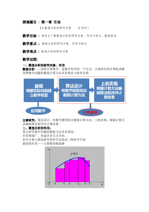
授课题目: 第一章引论§1数值分析的研究对象(1学时)教学目标: 使学生了解数值分析的研究对象、作用与特点、数值算法教学重点:数值分析的研究对象、作用与特点教学难点: 数值分析的研究对象教学过程:一、数值分析的研究对象、作用数值分析——也称计算数学,是数学科学的一个分支,主要研究用计算机求解各种数学问题的数值计算方法及其理论与软件实现.主要研究:算法设计,有数学模型给出数值计算方法;上机实现,根据计算方法编制算法程序并计算结果二、数值分析的作用:重点研究数学问题的数值方法及其理论。
作用领域广,形成许多交叉学科。
科学计算与理论研究和科学实验是三种科学手段最重要作用——计算模型数值解三、数值分析的特点面向计算机,根据计算机特点提供有效算法。
有可靠的理论分析,能任意逼近并达到精度要求。
要有好的计算复杂性——时间和空间复杂性。
要有数值实验。
证明其有效性。
练习:思考:作业:教学反思:授课题目: §2 数值计算的误差(1学时)教学目标: 使学生掌握误差、有效数字及其关系、误差估计教学重点:误差、有效数字及其关系、误差估计教学难点: 误差估计教学过程:误差来源与分类截断误差例如,可微函数f(x)的泰勒(Taylor)多项式则数值方法的截断误差是舍入误差例如,用3.14159代替π,产生的误差●由原始数据或机器中的十进制数转化为二进制数产生的初始误差。
●在用计算机做数值计算时,受计算机字长的限制产生的误差。
误差与有效数字定义1 设x为准确值,x*为x的一个近似值,称为近似值的绝对误差,简称误差。
通常准确值x 是未知的,因此误差e *也是未知的。
若能根据测量工具或计算情况估计出误差绝对值的一个上界,即则ε*叫做近似值的误差限 也可表示成把近似值的误差e *与准确值x 的比值称为近似值x *的相对误差,记作e r ∗它的绝对值上界叫做相对误差限,记作εr ∗,定义2 若近似值x *的误差限是某一位的半个单位,该位到x *的第一位非零数字共有n 位,就说x * 有n 位有效数字.其中a i 是0到9中的一个数字,m 为整数,且定理1设近似数x *表示为x x e -=*****ε≤-=x x e *,***εε+≤≤-x x x .**ε±=x x x xx x e -=*******x xx x e e r-==.***x r εε=其中a i 是0到9中的一个数字,m 为整数,若x *具有n 位有效数字,则其相对误差限为反之,若x *的相对误差限则x *具有n 位有效数字。
数值分析习题(含标准答案)
]第一章 绪论姓名 学号 班级习题主要考察点:有效数字的计算、计算方法的比较选择、误差和误差限的计算。
1若误差限为5105.0-⨯,那么近似数有几位有效数字(有效数字的计算) 解:2*103400.0-⨯=x ,325*10211021---⨯=⨯≤-x x 故具有3位有效数字。
2 14159.3=π具有4位有效数字的近似值是多少(有效数字的计算) 解:10314159.0⨯= π,欲使其近似值*π具有4位有效数字,必需!41*1021-⨯≤-ππ,3*310211021--⨯+≤≤⨯-πππ,即14209.314109.3*≤≤π即取( , )之间的任意数,都具有4位有效数字。
3已知2031.1=a ,978.0=b 是经过四舍五入后得到的近似值,问b a +,b a ⨯有几位有效数字(有效数字的计算)解:3*1021-⨯≤-aa ,2*1021-⨯≤-b b ,而1811.2=+b a ,1766.1=⨯b a 2123****102110211021)()(---⨯≤⨯+⨯≤-+-≤+-+b b a a b a b a故b a +至少具有2位有效数字。
2123*****10210065.01022031.1102978.0)()(---⨯≤=⨯+⨯≤-+-≤-b b a a a b b a ab 故b a ⨯至少具有2位有效数字。
4设0>x ,x 的相对误差为δ,求x ln 的误差和相对误差(误差的计算)~解:已知δ=-**xx x ,则误差为 δ=-=-***ln ln xx x x x则相对误差为******ln ln 1ln ln ln xxx x xxx x δ=-=-5测得某圆柱体高度h 的值为cm h 20*=,底面半径r 的值为cm r 5*=,已知cm h h 2.0||*≤-,cm r r 1.0||*≤-,求圆柱体体积h r v2π=的绝对误差限与相对误差限。
(误差限的计算)解:*2******2),(),(h h r r r h r r h v r h v -+-≤-ππ绝对误差限为πππ252.051.02052)5,20(),(2=⨯⋅+⨯⋅⋅⋅≤-v r h v相对误差限为%420120525)5,20()5,20(),(2==⋅⋅≤-ππv v r h v 6设x 的相对误差为%a ,求nx y =的相对误差。
数值分析第二版(丁丽娟)答案
练习: 第一章
答案
练习二 练习三
练习四
1、 什么是幂法?它收敛到矩阵 A 的哪个特征向量? 若 A 的按模最大的特征值是单根,用幂法求此特征 值的收敛速度由什么量来决定?怎样改进幂法的收敛速度?
2、 反幂法收敛到矩阵的哪个特征向量? 在幂法或者反ห้องสมุดไป่ตู้法中,为什么每步都要将迭代向量规范化?
,求差商 (2)
例6 设
,
Hermite 插值多项式 其误差余项。
,满足
例7已知函数 的取值如下,
x
-1
y
-1
y’
4
,求函数
在区间
上的
,
。并写出
0
1
3
1
3
31
28
求其三次样条插值函数
,并求出
在 -0.5 和2 的近似值。
练习六
1、解:由
由 10(1)解:
第七章答案 得
得
。
0
1
0 0.235294 0.400000 0.4800 0.5
16(3)解: 将
代入得
,
解得:
对于求积公式 有2次代数精确度。
,
,将
代入不成立,因此公式具
19(1)解:
将
代入得
将
代入得
将
代入得
因此其代数精确度为2次,不是 Gauss 型求积公式。
21、解:三点公式
16.007498295841852 16.002385008517887
16.002177786576915 16.00069286350589
则开根号得 4.000114446266071 4.000272214059553 4.000086607000640
数值分析课后习题及答案
第一章 绪论(12) 第二章 插值法(40-42)2、当2,1,1-=x 时,4,3,0)(-=x f ,求)(x f 的二次插值多项式。
[解]372365)1(34)23(21)12)(12()1)(1(4)21)(11()2)(1()3()21)(11()2)(1(0))(())(())(())(())(())(()(2221202102210120120102102-+=-++--=+-+-⨯+------⨯-+-+-+⨯=----+----+----=x x x x x x x x x x x x x x x x x x x y x x x x x x x x y x x x x x x x x y x L 。
3、给出x x f ln )(=的数值表用线性插值及二次插值计算54.0ln 的近似值。
X 0.4 0.5 0.6 0.7 0.8 x ln -0.916291 -0.693147 -0.510826 -0.357765 -0.223144[解]若取5.00=x ,6.01=x ,则693147.0)5.0()(00-===f x f y ,510826.0)6.0()(11-===f x f y ,则604752.182321.1)5.0(10826.5)6.0(93147.65.06.05.0510826.06.05.06.0693147.0)(010110101-=---=--⨯---⨯-=--+--=x x x x x x x x x y x x x x y x L ,从而6202186.0604752.19845334.0604752.154.082321.1)54.0(1-=-=-⨯=L 。
若取4.00=x ,5.01=x ,6.02=x ,则916291.0)4.0()(00-===f x f y ,693147.0)5.0()(11-===f x f y ,510826.0)6.0()(22-===f x f y ,则 217097.2068475.404115.2)2.09.0(5413.25)24.0(3147.69)3.01.1(81455.45)5.06.0)(4.06.0()5.0)(4.0()510826.0()6.05.0)(4.05.0()6.0)(4.0()693147.0()6.04.0)(5.04.0()6.0)(5.0(916291.0))(())(())(())(())(())(()(22221202102210120120102102-+-=+--+-⨯++-⨯-=----⨯-+----⨯-+----⨯-=----+----+----=x x x x x x x x x x x x x x x x x x x x x x y x x x x x x x x y x x x x x x x x y x L ,从而61531984.0217097.21969765.259519934.0217097.254.0068475.454.004115.2)54.0(22-=-+-=-⨯+⨯-=L补充题:1、令00=x ,11=x ,写出x e x y -=)(的一次插值多项式)(1x L ,并估计插值余项。
数值分析(计算方法)总结
第一章绪论误差来源:模型误差、观测误差、截断误差(方法误差)、舍入误差是的绝对误差,是的误差,为的绝对误差限(或误差限)为的相对误差,当较小时,令相对误差绝对值得上限称为相对误差限记为:即:绝对误差有量纲,而相对误差无量纲若近似值的绝对误差限为某一位上的半个单位,且该位直到的第一位非零数字共有n位,则称近似值有n位有效数字,或说精确到该位。
例:设x==3。
1415926…那么,则有效数字为1位,即个位上的3,或说精确到个位.科学计数法:记有n位有效数字,精确到。
由有效数字求相对误差限:设近似值有n位有效数字,则其相对误差限为由相对误差限求有效数字:设近似值的相对误差限为为则它有n位有效数字令1.x+y近似值为和的误差(限)等于误差(限)的和2.x-y近似值为3.xy近似值为4.1.避免两相近数相减2.避免用绝对值很小的数作除数3.避免大数吃小数4.尽量减少计算工作量第二章非线性方程求根1。
逐步搜索法设f (a) <0, f (b)〉 0,有根区间为 (a, b),从x0=a出发,按某个预定步长(例如h=(b-a)/N)一步一步向右跨,每跨一步进行一次根的搜索,即判别f(x k)=f(a+kh)的符号,若f(x k)〉0(而f(x k-1)<0),则有根区间缩小为[x k-1,x k] (若f(x k)=0,x k即为所求根),然后从x k—1出发,把搜索步长再缩小,重复上面步骤,直到满足精度:|x k—x k-1|< 为止,此时取x*≈(x k+x k-1)/2作为近似根.2。
二分法设f(x)的有根区间为[a,b]= [a0,b0], f(a)<0,f(b)〉0。
将[a0,b0]对分,中点x0= ((a0+b0)/2),计算f(x0)。
3.比例法一般地,设 [a k,b k]为有根区间,过(a k,f(a k))、 (b k, f(b k))作直线,与x轴交于一点x k,则:1.试位法每次迭代比二分法多算一次乘法,而且不保证收敛.2。
- 1、下载文档前请自行甄别文档内容的完整性,平台不提供额外的编辑、内容补充、找答案等附加服务。
- 2、"仅部分预览"的文档,不可在线预览部分如存在完整性等问题,可反馈申请退款(可完整预览的文档不适用该条件!)。
- 3、如文档侵犯您的权益,请联系客服反馈,我们会尽快为您处理(人工客服工作时间:9:00-18:30)。
Chapter 1 Solving Nonlinear EquationTopics: 1. Interval Halving(Bisection) 2. Linear Interpolating Methods 3. Newton’s Method 4. Muller’s Method 5. Fixed-Point Iteration 6. Nonlinear SystemA SurveyOne of the most frequently occurring problems in scientific work is to find the roots of equations of the form Function The roots, or zeros of the function Example:We know thatBut how about the equationIt’s not easy to obtain the exact roots. In general, we hope to get only approximate solutions.“Approximate solution” means a point small, or is closed to a solution,for which of the equationisBut the concept of an “approximate solution” is rather fuzzy. There are many difficulties that we will encounter. All these will be shown in the following section.1. Interval Halving(Bisection, Binarysearching Method)Suppose with is a continuous function defined on the interval and of opposite sign, then there exits a number , insuch that Bisectionf ( x1 )px11x2 f ( x2 )x2 Letis the middle point of3 Letis the middle point ofThe middle point ……is more closer toWe are back to the functionMATLAB command: >>f=inline(‘3*x+sin(x)-exp(x)’) >>fplot(f,[0,2]); grid on From the figure we know one root is in and another is inAlgorithm: Repeat Set If Set Else Set Until End If. thenProgram: click hereThe Error If f(x) is continuous in [a, b], which actually bracket a root. Note that we have the following relation ship. Times 1 2 3 … n It’s clear the root . So, the error ……. Interval lengthFrom, we getHere are some values aboutandn 5 10 20 30 Disadvantage: Interval Halving method is slow to converge. The speed of convergence is linear.Exercises:Find an approximation to Bisection Algorithm. correct to within by using2. Linear interpolation Methods1.The secant methodLet be the initial points which are near to the root. From the figure we haveThen,If we repeat this, we have:Each newly computed value should be nearer to the root, so we always use the last two computed points. But after the first iteration, we need to check whether is closer to the root than Example:Use secant method for . How to do this?From the figure, we know there is a root in the interval [0,1]. Of course we can use 0 and 1 as the initial points, and 0 is closer to the root than 1.Table Iteration 1 2 3 4 5 1 0 0.4709896 0.3722771 0.3599043 x0 0 0.4709896 0.3722771 0.3599043 0.3604239 x1 x2 0.4709896 0.3722771 0.3599043 0.3604239 0.3604217 F(x2) 0.2651588 2.953367E-02 -1.294787E-03 5.552969E-0.6 3.554221E-08The exact value is 0.36042170296…. Fewer iterations are required compared to bisection!Algorithm: are given. Compute If Swap End If Repeat Set Set Until Or then andA pathological caseThe two initial points should be close to the root as much as possible! Plotting the function can help you to choose the initial points!2. Linear Interpolation (False Position) A way to avoid this pathology is to ensure that the root is bracketed between the two starting values and remains between the successive pairs.Choose the starting value Then use the formula, such thatto get. The next step is to check the root is in the interval3. Newton’s MethodSuppose that such that series of at and , . Let be an approximation to is “small”. Consider the Taylorwherelies betweenand. So,Sinceis small, the term involvingis much smaller, soSolving for x givesStarting with an initial approximation, the formulagenerates the approximate sequence. This is Newton’s Method.This formula also can be derive from the figure.Then,Repeat this work, we can get the schemeExample: Use Newton’s method forWe need compute, and need a initial value of x.We can get this derivative in Matlab: >> fx=sym(‘3*x+sin(x)-exp(x)’) >>dfx=diff(fx) dfx=3+cos(x)-exp(x) If we begin with , we haveThe exact value is 0.36042170296….Compare with other methods Bisection Initial value After 5 Iterations # of significant digital Example: Use Newton’s method to find the value of It equals to find the positive root of . 0.34375 1 False Position Secant method Newton’s method x0=0 -31 x0=1 -12x0=0, x1=1 0.360433 4 0.360422 5By using Newton’s method we haveWe can prove that x converge to the exact value for any (See Numerical Analysis (in Chinese), Li Qingyang, 278-279) Algorithm: For any Repeat Set Set Until Or (tolerance) ,.In some cases, the result does not converge to the root with Newton’s method . Rootûx û x xü0 0 0The conclusion is that the convergence depends on the choosing of.Relating Newton’s Method to Other Methods Recall the formula of the linear interpolation:We rewrite it to the form Difference QuotientSuppose that thatis very closed toandis continuous. We note. By taking the limit we haveThe definition of the derivativeHence,Newton’s MethodIn fact, the difference quotient can be regard as an approximation to the derivative. A simplified newton’s method (see Numerical Analysis, Li Qingyang, P280)Newton's descent method (see Numerical Analysis, Li Qingyang, P281)The parameteris chosen such that4. Muller’s Method (Parabola Method)Previous methods: straight line Muller’s methods: quadratic polynomialA second-degree polynomial is made to fit three points near a root, x0, x1, x2, with x0 between x1 and x2.Assume the quadratic polynomial has the formLetLetting,we can obtain a, b and c:So,Which root we should choose? And how to judge? The one nearest to x0.If b>0, choose +; If b<0, choose -; If b=0, choose either. When we get the root v, we may choose three points as the initial points for the next approximation. There are some cases to discuss. root rootX2, root, x0X0, root, x1Algorithm: are given and RepeatSet Set Compute: ;If b>=0, then letElse, let End If If x>x0, then let x2=x0, x0=x; Else let x1=x0, x0=x; End If. Until4. Fixed-Point IterationTheorem: Suppose that is a real-value function, defined and for , continuous on a bounded closed interval [a, b], and let all . Then, there exists in [a, b] , such that .is called a fixed-point of the functionIf, in addition, withexits on (a, b) and a positive constant k<1 existsthen the fixed point in [a, b] is unique. Proof If g(a)=a or g(b)=b, then g has a fixed point. If not, then g(a)>a and g(b)<b. The function h(x)=g(x)-x is continuous on [a, b] withThen there exists point sincefor which.Is a fixedSuppose , in addition, that points in [a, b]. If , thenand that p and q are both fixedThus,which is a contradiction. So, p=q and the fixed point in [a, b] is unique. Fixed-point iteration To approximate the fixed point of and generate the sequence , we choose an initial approximation by letting . IfAnd a solution to iteration.is obtained, this technique is called fixed-pointThe figure illustrates the algorithm.Example(P54): (The roots are -1 and 3.) Form1:We will find if obtain the fixed point., also,Fig.. . Then we can usetoIt converges to 3. It converges to 3.Form2:We start the iteration withFig.It converges to -1. Form3:We start the iteration again withFig.It’s diverging.Theorem (Fixed-Point Theorem)Let in addition, that with be such that , for all x in [a, b]. Suppose, existsexists on (a, b) and that a constantThen, for any numberin [a, b], the sequence defined byConverges to the unique fixed point. We just need prove converges to the fixed point r.Order of ConvergenceDefinition Supposefor measuring how rapidly a sequence converges., withis a sequence that converges to and exists withfor all n. If positive constantthen Specially,converges toof order, with asymptotic error constant k.1 If 1 If,the sequence is linearly convergent. ,the sequence is quadratically convergent.SpeedSome Theory (P58)1. Convergence order of Fixed-point iterationSuppose that R is the true value of the root, we havewhere Then,is betweenand, and, since.Hence, if error constant, fixed-point iteration is linear convergent with asymptotic .2. Convergence order of Newton’s MethodAccording to the theorem, Newton’s iteration schemewill converge if .Then,and Now we expand, where R is the exact value of the root. as a Taylor series in terms of .wherelies within. So,.Hence,since . Also, is continuous and strictly bounded by K in the neighborhood of R, we have,That means if How about ?, Newton’s method is quadratically convergent.3. Convergence order of Secant MethodPizer (1975) shows that the order of convergence of the secant method isMultiple RootsDisadvantages of the methods we have described: 1. Do not work well for multiple roots. We will only get a slow convergence. 2. Imprecision. The curve is very flat near the multiple root—f’(x) will always be zero, that is, the program cannot distinguish which x-value is really the root.Remedies for Multiple Root with Newton’s MethodWe have discussed thatwhere, if R is the simple root. However, if f(x) has a root ofmultiplicity k at x=R, we havewhere Q(x) has no root R. Obviously,but.Does g’(R) still equal 0 ? We are not sure.We present a different formulation of Newton’s method:As before, at. We have,We see that, and now the new iteration converges quadraticallyat a multiple root. But we should know k in advance.Nearly Multiple RootsAccelerating Convergence Aitken accelerationSuppose there exists a constant K such thatwhere the error, R is the true value of the root. Then,Solving the equation givesWe will get a new sequenceby definingDefinition For a given sequence is defined by,the forward differenceHigher power, are defined byThis definition implies thatSo, the formula forcan be written asWe can proveThis means the sequence original sequence .converges more rapidly than does theExercise Give the algorithm of Aitken acceleration.Algorithm:is given as the initial approximation. Repeat SetUntil6. Nonlinear SystemIn fact, the situation of nonlinear system is more difficult.We note it to Giving an approximation. ,w to Taylor series at , we expand the , and select thefunction with many variables linear parts to obtainSolving the equation and noting it togives,Whereis the Jacobi matrix with the formExample Use Newton’s method forWe use the initial approximationto iterate, the result is:N 01 2 3 4 5 6x 1.0000000 2.1893260 1.8505896 1.7801611 1.7776747 1.7776719 1.7776719y 1.0000000 1.5984751 1.4442514 1.4244359 1.4239609 1.4239605 1.4239605z 1.00000000 1.3939006 1.2782240 1.2392924 1.2374738 1.2374711 1.2374711。