Speaker Diarization For Multi-Microphone Meetings Using only BetweenChannel Differences
Multi-scale structural similarity for image quality assesment
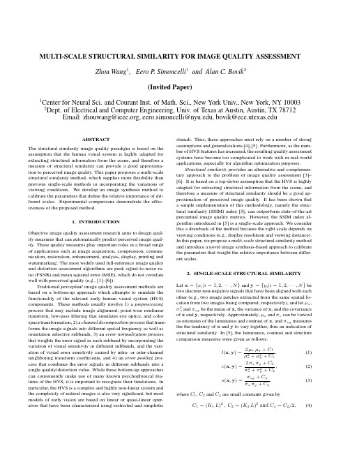
MULTI-SCALE STRUCTURAL SIMILARITY FOR IMAGE QUALITY ASSESSMENT Zhou Wang1,Eero P.Simoncelli1and Alan C.Bovik2(Invited Paper)1Center for Neural Sci.and Courant Inst.of Math.Sci.,New York Univ.,New York,NY10003 2Dept.of Electrical and Computer Engineering,Univ.of Texas at Austin,Austin,TX78712 Email:zhouwang@,eero.simoncelli@,bovik@ABSTRACTThe structural similarity image quality paradigm is based on the assumption that the human visual system is highly adapted for extracting structural information from the scene,and therefore a measure of structural similarity can provide a good approxima-tion to perceived image quality.This paper proposes a multi-scale structural similarity method,which supplies moreflexibility than previous single-scale methods in incorporating the variations of viewing conditions.We develop an image synthesis method to calibrate the parameters that define the relative importance of dif-ferent scales.Experimental comparisons demonstrate the effec-tiveness of the proposed method.1.INTRODUCTIONObjective image quality assessment research aims to design qual-ity measures that can automatically predict perceived image qual-ity.These quality measures play important roles in a broad range of applications such as image acquisition,compression,commu-nication,restoration,enhancement,analysis,display,printing and watermarking.The most widely used full-reference image quality and distortion assessment algorithms are peak signal-to-noise ra-tio(PSNR)and mean squared error(MSE),which do not correlate well with perceived quality(e.g.,[1]–[6]).Traditional perceptual image quality assessment methods are based on a bottom-up approach which attempts to simulate the functionality of the relevant early human visual system(HVS) components.These methods usually involve1)a preprocessing process that may include image alignment,point-wise nonlinear transform,low-passfiltering that simulates eye optics,and color space transformation,2)a channel decomposition process that trans-forms the image signals into different spatial frequency as well as orientation selective subbands,3)an error normalization process that weights the error signal in each subband by incorporating the variation of visual sensitivity in different subbands,and the vari-ation of visual error sensitivity caused by intra-or inter-channel neighboring transform coefficients,and4)an error pooling pro-cess that combines the error signals in different subbands into a single quality/distortion value.While these bottom-up approaches can conveniently make use of many known psychophysical fea-tures of the HVS,it is important to recognize their limitations.In particular,the HVS is a complex and highly non-linear system and the complexity of natural images is also very significant,but most models of early vision are based on linear or quasi-linear oper-ators that have been characterized using restricted and simplistic stimuli.Thus,these approaches must rely on a number of strong assumptions and generalizations[4],[5].Furthermore,as the num-ber of HVS features has increased,the resulting quality assessment systems have become too complicated to work with in real-world applications,especially for algorithm optimization purposes.Structural similarity provides an alternative and complemen-tary approach to the problem of image quality assessment[3]–[6].It is based on a top-down assumption that the HVS is highly adapted for extracting structural information from the scene,and therefore a measure of structural similarity should be a good ap-proximation of perceived image quality.It has been shown that a simple implementation of this methodology,namely the struc-tural similarity(SSIM)index[5],can outperform state-of-the-art perceptual image quality metrics.However,the SSIM index al-gorithm introduced in[5]is a single-scale approach.We consider this a drawback of the method because the right scale depends on viewing conditions(e.g.,display resolution and viewing distance). In this paper,we propose a multi-scale structural similarity method and introduce a novel image synthesis-based approach to calibrate the parameters that weight the relative importance between differ-ent scales.2.SINGLE-SCALE STRUCTURAL SIMILARITYLet x={x i|i=1,2,···,N}and y={y i|i=1,2,···,N}be two discrete non-negative signals that have been aligned with each other(e.g.,two image patches extracted from the same spatial lo-cation from two images being compared,respectively),and letµx,σ2x andσxy be the mean of x,the variance of x,and the covariance of x and y,respectively.Approximately,µx andσx can be viewed as estimates of the luminance and contrast of x,andσxy measures the the tendency of x and y to vary together,thus an indication of structural similarity.In[5],the luminance,contrast and structure comparison measures were given as follows:l(x,y)=2µxµy+C1µ2x+µ2y+C1,(1)c(x,y)=2σxσy+C2σ2x+σ2y+C2,(2)s(x,y)=σxy+C3σxσy+C3,(3) where C1,C2and C3are small constants given byC1=(K1L)2,C2=(K2L)2and C3=C2/2,(4)Fig.1.Multi-scale structural similarity measurement system.L:low-passfiltering;2↓:downsampling by2. respectively.L is the dynamic range of the pixel values(L=255for8bits/pixel gray scale images),and K1 1and K2 1aretwo scalar constants.The general form of the Structural SIMilarity(SSIM)index between signal x and y is defined as:SSIM(x,y)=[l(x,y)]α·[c(x,y)]β·[s(x,y)]γ,(5)whereα,βandγare parameters to define the relative importanceof the three components.Specifically,we setα=β=γ=1,andthe resulting SSIM index is given bySSIM(x,y)=(2µxµy+C1)(2σxy+C2)(µ2x+µ2y+C1)(σ2x+σ2y+C2),(6)which satisfies the following conditions:1.symmetry:SSIM(x,y)=SSIM(y,x);2.boundedness:SSIM(x,y)≤1;3.unique maximum:SSIM(x,y)=1if and only if x=y.The universal image quality index proposed in[3]corresponds to the case of C1=C2=0,therefore is a special case of(6).The drawback of such a parameter setting is that when the denominator of Eq.(6)is close to0,the resulting measurement becomes unsta-ble.This problem has been solved successfully in[5]by adding the two small constants C1and C2(calculated by setting K1=0.01 and K2=0.03,respectively,in Eq.(4)).We apply the SSIM indexing algorithm for image quality as-sessment using a sliding window approach.The window moves pixel-by-pixel across the whole image space.At each step,the SSIM index is calculated within the local window.If one of the image being compared is considered to have perfect quality,then the resulting SSIM index map can be viewed as the quality map of the other(distorted)image.Instead of using an8×8square window as in[3],a smooth windowing approach is used for local statistics to avoid“blocking artifacts”in the quality map[5].Fi-nally,a mean SSIM index of the quality map is used to evaluate the overall image quality.3.MULTI-SCALE STRUCTURAL SIMILARITY3.1.Multi-scale SSIM indexThe perceivability of image details depends the sampling density of the image signal,the distance from the image plane to the ob-server,and the perceptual capability of the observer’s visual sys-tem.In practice,the subjective evaluation of a given image varies when these factors vary.A single-scale method as described in the previous section may be appropriate only for specific settings.Multi-scale method is a convenient way to incorporate image de-tails at different resolutions.We propose a multi-scale SSIM method for image quality as-sessment whose system diagram is illustrated in Fig. 1.Taking the reference and distorted image signals as the input,the system iteratively applies a low-passfilter and downsamples thefiltered image by a factor of2.We index the original image as Scale1, and the highest scale as Scale M,which is obtained after M−1 iterations.At the j-th scale,the contrast comparison(2)and the structure comparison(3)are calculated and denoted as c j(x,y) and s j(x,y),respectively.The luminance comparison(1)is com-puted only at Scale M and is denoted as l M(x,y).The overall SSIM evaluation is obtained by combining the measurement at dif-ferent scales usingSSIM(x,y)=[l M(x,y)]αM·Mj=1[c j(x,y)]βj[s j(x,y)]γj.(7)Similar to(5),the exponentsαM,βj andγj are used to ad-just the relative importance of different components.This multi-scale SSIM index definition satisfies the three conditions given in the last section.It also includes the single-scale method as a spe-cial case.In particular,a single-scale implementation for Scale M applies the iterativefiltering and downsampling procedure up to Scale M and only the exponentsαM,βM andγM are given non-zero values.To simplify parameter selection,we letαj=βj=γj forall j’s.In addition,we normalize the cross-scale settings such thatMj=1γj=1.This makes different parameter settings(including all single-scale and multi-scale settings)comparable.The remain-ing job is to determine the relative values across different scales. Conceptually,this should be related to the contrast sensitivity func-tion(CSF)of the HVS[7],which states that the human visual sen-sitivity peaks at middle frequencies(around4cycles per degree of visual angle)and decreases along both high-and low-frequency directions.However,CSF cannot be directly used to derive the parameters in our system because it is typically measured at the visibility threshold level using simplified stimuli(sinusoids),but our purpose is to compare the quality of complex structured im-ages at visible distortion levels.3.2.Cross-scale calibrationWe use an image synthesis approach to calibrate the relative impor-tance of different scales.In previous work,the idea of synthesizing images for subjective testing has been employed by the“synthesis-by-analysis”methods of assessing statistical texture models,inwhich the model is used to generate a texture with statistics match-ing an original texture,and a human subject then judges the sim-ilarity of the two textures [8]–[11].A similar approach has also been qualitatively used in demonstrating quality metrics in [5],[12],though quantitative subjective tests were not conducted.These synthesis methods provide a powerful and efficient means of test-ing a model,and have the added benefit that the resulting images suggest improvements that might be made to the model[11].M )distortion level (MSE)12345Fig.2.Demonstration of image synthesis approach for cross-scale calibration.Images in the same row have the same MSE.Images in the same column have distortions only in one specific scale.Each subject was asked to select a set of images (one from each scale),having equal quality.As an example,one subject chose the marked images.For a given original 8bits/pixel gray scale test image,we syn-thesize a table of distorted images (as exemplified by Fig.2),where each entry in the table is an image that is associated witha specific distortion level (defined by MSE)and a specific scale.Each of the distorted image is created using an iterative procedure,where the initial image is generated by randomly adding white Gaussian noise to the original image and the iterative process em-ploys a constrained gradient descent algorithm to search for the worst images in terms of SSIM measure while constraining MSE to be fixed and restricting the distortions to occur only in the spec-ified scale.We use 5scales and 12distortion levels (range from 23to 214)in our experiment,resulting in a total of 60images,as demonstrated in Fig.2.Although the images at each row has the same MSE with respect to the original image,their visual quality is significantly different.Thus the distortions at different scales are of very different importance in terms of perceived image quality.We employ 10original 64×64images with different types of con-tent (human faces,natural scenes,plants,man-made objects,etc.)in our experiment to create 10sets of distorted images (a total of 600distorted images).We gathered data for 8subjects,including one of the authors.The other subjects have general knowledge of human vision but did not know the detailed purpose of the study.Each subject was shown the 10sets of test images,one set at a time.The viewing dis-tance was fixed to 32pixels per degree of visual angle.The subject was asked to compare the quality of the images across scales and detect one image from each of the five scales (shown as columns in Fig.2)that the subject believes having the same quality.For example,one subject chose the images marked in Fig.2to have equal quality.The positions of the selected images in each scale were recorded and averaged over all test images and all subjects.In general,the subjects agreed with each other on each image more than they agreed with themselves across different images.These test results were normalized (sum to one)and used to calculate the exponents in Eq.(7).The resulting parameters we obtained are β1=γ1=0.0448,β2=γ2=0.2856,β3=γ3=0.3001,β4=γ4=0.2363,and α5=β5=γ5=0.1333,respectively.4.TEST RESULTSWe test a number of image quality assessment algorithms using the LIVE database (available at [13]),which includes 344JPEG and JPEG2000compressed images (typically 768×512or similar size).The bit rate ranges from 0.028to 3.150bits/pixel,which allows the test images to cover a wide quality range,from in-distinguishable from the original image to highly distorted.The mean opinion score (MOS)of each image is obtained by averag-ing 13∼25subjective scores given by a group of human observers.Eight image quality assessment models are being compared,in-cluding PSNR,the Sarnoff model (JNDmetrix 8.0[14]),single-scale SSIM index with M equals 1to 5,and the proposed multi-scale SSIM index approach.The scatter plots of MOS versus model predictions are shown in Fig.3,where each point represents one test image,with its vertical and horizontal axes representing its MOS and the given objective quality score,respectively.To provide quantitative per-formance evaluation,we use the logistic function adopted in the video quality experts group (VQEG)Phase I FR-TV test [15]to provide a non-linear mapping between the objective and subjective scores.After the non-linear mapping,the linear correlation coef-ficient (CC),the mean absolute error (MAE),and the root mean squared error (RMS)between the subjective and objective scores are calculated as measures of prediction accuracy .The prediction consistency is quantified using the outlier ratio (OR),which is de-Table1.Performance comparison of image quality assessment models on LIVE JPEG/JPEG2000database[13].SS-SSIM: single-scale SSIM;MS-SSIM:multi-scale SSIM;CC:non-linear regression correlation coefficient;ROCC:Spearman rank-order correlation coefficient;MAE:mean absolute error;RMS:root mean squared error;OR:outlier ratio.Model CC ROCC MAE RMS OR(%)PSNR0.9050.901 6.538.4515.7Sarnoff0.9560.947 4.66 5.81 3.20 SS-SSIM(M=1)0.9490.945 4.96 6.25 6.98 SS-SSIM(M=2)0.9630.959 4.21 5.38 2.62 SS-SSIM(M=3)0.9580.956 4.53 5.67 2.91 SS-SSIM(M=4)0.9480.946 4.99 6.31 5.81 SS-SSIM(M=5)0.9380.936 5.55 6.887.85 MS-SSIM0.9690.966 3.86 4.91 1.16fined as the percentage of the number of predictions outside the range of±2times of the standard deviations.Finally,the predic-tion monotonicity is measured using the Spearman rank-order cor-relation coefficient(ROCC).Readers can refer to[15]for a more detailed descriptions of these measures.The evaluation results for all the models being compared are given in Table1.From both the scatter plots and the quantitative evaluation re-sults,we see that the performance of single-scale SSIM model varies with scales and the best performance is given by the case of M=2.It can also be observed that the single-scale model tends to supply higher scores with the increase of scales.This is not surprising because image coding techniques such as JPEG and JPEG2000usually compressfine-scale details to a much higher degree than coarse-scale structures,and thus the distorted image “looks”more similar to the original image if evaluated at larger scales.Finally,for every one of the objective evaluation criteria, multi-scale SSIM model outperforms all the other models,includ-ing the best single-scale SSIM model,suggesting a meaningful balance between scales.5.DISCUSSIONSWe propose a multi-scale structural similarity approach for image quality assessment,which provides moreflexibility than single-scale approach in incorporating the variations of image resolution and viewing conditions.Experiments show that with an appropri-ate parameter settings,the multi-scale method outperforms the best single-scale SSIM model as well as state-of-the-art image quality metrics.In the development of top-down image quality models(such as structural similarity based algorithms),one of the most challeng-ing problems is to calibrate the model parameters,which are rather “abstract”and cannot be directly derived from simple-stimulus subjective experiments as in the bottom-up models.In this pa-per,we used an image synthesis approach to calibrate the param-eters that define the relative importance between scales.The im-provement from single-scale to multi-scale methods observed in our tests suggests the usefulness of this novel approach.However, this approach is still rather crude.We are working on developing it into a more systematic approach that can potentially be employed in a much broader range of applications.6.REFERENCES[1] A.M.Eskicioglu and P.S.Fisher,“Image quality mea-sures and their performance,”IEEE munications, vol.43,pp.2959–2965,Dec.1995.[2]T.N.Pappas and R.J.Safranek,“Perceptual criteria for im-age quality evaluation,”in Handbook of Image and Video Proc.(A.Bovik,ed.),Academic Press,2000.[3]Z.Wang and A.C.Bovik,“A universal image quality in-dex,”IEEE Signal Processing Letters,vol.9,pp.81–84,Mar.2002.[4]Z.Wang,H.R.Sheikh,and A.C.Bovik,“Objective videoquality assessment,”in The Handbook of Video Databases: Design and Applications(B.Furht and O.Marques,eds.), pp.1041–1078,CRC Press,Sept.2003.[5]Z.Wang,A.C.Bovik,H.R.Sheikh,and E.P.Simon-celli,“Image quality assessment:From error measurement to structural similarity,”IEEE Trans.Image Processing,vol.13, Jan.2004.[6]Z.Wang,L.Lu,and A.C.Bovik,“Video quality assessmentbased on structural distortion measurement,”Signal Process-ing:Image Communication,special issue on objective video quality metrics,vol.19,Jan.2004.[7] B.A.Wandell,Foundations of Vision.Sinauer Associates,Inc.,1995.[8]O.D.Faugeras and W.K.Pratt,“Decorrelation methods oftexture feature extraction,”IEEE Pat.Anal.Mach.Intell., vol.2,no.4,pp.323–332,1980.[9] A.Gagalowicz,“A new method for texturefields synthesis:Some applications to the study of human vision,”IEEE Pat.Anal.Mach.Intell.,vol.3,no.5,pp.520–533,1981. [10] D.Heeger and J.Bergen,“Pyramid-based texture analy-sis/synthesis,”in Proc.ACM SIGGRAPH,pp.229–238,As-sociation for Computing Machinery,August1995.[11]J.Portilla and E.P.Simoncelli,“A parametric texture modelbased on joint statistics of complex wavelet coefficients,”Int’l J Computer Vision,vol.40,pp.49–71,Dec2000. [12]P.C.Teo and D.J.Heeger,“Perceptual image distortion,”inProc.SPIE,vol.2179,pp.127–141,1994.[13]H.R.Sheikh,Z.Wang, A. C.Bovik,and L.K.Cormack,“Image and video quality assessment re-search at LIVE,”/ research/quality/.[14]Sarnoff Corporation,“JNDmetrix Technology,”http:///products_services/video_vision/jndmetrix/.[15]VQEG,“Final report from the video quality experts groupon the validation of objective models of video quality assess-ment,”Mar.2000./.PSNRM O SSarnoffM O S(a)(b)Single−scale SSIM (M=1)M O SSingle−scale SSIM (M=2)M O S(c)(d)Single−scale SSIM (M=3)M O SSingle−scale SSIM (M=4)M O S(e)(f)Single−scale SSIM (M=5)M O SMulti−scale SSIMM O S(g)(h)Fig.3.Scatter plots of MOS versus model predictions.Each sample point represents one test image in the LIVE JPEG/JPEG2000image database [13].(a)PSNR;(b)Sarnoff model;(c)-(g)single-scale SSIM method for M =1,2,3,4and 5,respectively;(h)multi-scale SSIM method.。
语音识别参考文献
语音识别参考文献语音识别是一项广泛应用于人机交互、语音翻译、智能助手等领域的技术。
它的目标是将人的语音输入转化为可理解和处理的文本数据。
随着人工智能和机器学习的发展,语音识别技术也得到了极大的提升和应用。
在语音识别领域,有许多经典的参考文献和研究成果。
以下是一些值得参考和研究的文献:1. Xiong, W., Droppo, J., Huang, X., Seide, F., Seltzer, M., Stolcke, A., & Yu, D. (2016). Achieving human parity in conversational speech recognition. arXiv preprintarXiv:1610.05256.这篇文章介绍了微软团队在语音识别方面的研究成果,实现了与人类口语识别准确率相媲美的结果。
2. Hinton, G., Deng, L., Yu, D., Dahl, G. E., Mohamed, A. R., Jaitly, N., ... & Kingsbury, B. (2012). Deep neural networks for acoustic modeling in speech recognition: The shared views of four research groups. IEEE Signal processing magazine, 29(6), 82-97.这篇文章介绍了深度神经网络在语音识别中的应用和研究进展,对于理解当前主流的语音识别技术有很大的帮助。
3. Hinton, G., Deng, L., Li, D., & Dahl, G. E. (2012). Deep neural networks for speech recognition. IEEE Signal Processing Magazine, 29(6), 82-97.这篇文章是语音识别中的经典之作,介绍了深度神经网络在语音识别中的应用和优势。
《2024年基于麦克风阵列的声源定向系统的研究与实现》范文

《基于麦克风阵列的声源定向系统的研究与实现》篇一一、引言随着科技的不断发展,声源定向系统在多个领域的应用日益广泛,包括但不限于智能机器人、智能家居、音频处理以及军事应用等。
而基于麦克风阵列的声源定向系统是当前声源定位研究领域的热门话题。
本篇论文将详细介绍基于麦克风阵列的声源定向系统的研究与实现过程。
二、麦克风阵列技术概述麦克风阵列技术是一种利用多个麦克风组成的阵列系统,通过分析声波在空间中的传播特性,实现对声源的定位和定向。
该技术具有高精度、高效率、低成本的优点,广泛应用于音频处理和语音识别等领域。
三、声源定向系统原理基于麦克风阵列的声源定向系统主要依赖于声波传播的相位差和时间差原理。
当声波传播到麦克风阵列时,不同麦克风之间会接收到不同时间和幅度的声波信号,根据这些差异,可以确定声源的方向和位置。
四、系统设计与实现4.1 系统架构设计本系统采用分布式架构设计,包括硬件部分和软件部分。
硬件部分主要包括多个麦克风、信号处理模块和通信模块;软件部分则包括信号采集、预处理、特征提取、声源定位和定向等模块。
4.2 信号采集与预处理首先,通过麦克风阵列采集声波信号,并进行预处理,包括滤波、降噪等操作,以提高信噪比和定位精度。
4.3 特征提取与声源定位利用特征提取算法从预处理后的信号中提取出关键特征,如到达时间差(TDOA)等。
然后通过声源定位算法,如最小均方误差(LMS)算法等,实现对声源的精确定位。
4.4 声源定向与实现结果根据声源的位置信息,结合声音传播方向信息,实现对声源的定向。
本系统通过计算声音传播方向向量和阵列响应矩阵的关系,实现声源定向的精确输出。
同时,我们通过实验验证了系统的性能和准确性。
五、实验与结果分析5.1 实验环境与数据集我们采用多种环境下的实际录音数据作为实验数据集,包括室内、室外、嘈杂环境等场景。
实验环境包括多个不同布局的麦克风阵列系统。
5.2 实验结果与分析通过对实验数据的分析,我们发现本系统在各种环境下的声源定位和定向性能表现良好。
TEM8 Mini-lecture的技巧(上)(2)

2008年专业八级考试听力部分Mini-lecture录音文稿Good morning, everyone. Today’s lecture is about the popularity of English. As we all know,English is widely used in the world. Although English is NOT the language with t he largest number of native or “first” language speakers, it has really become a lingua franca.Then, what is a lingua franca? The term refers to a language which is widely adopted for communication between two speakers whose native language s are different from each other’s, and where one or both speakers are using it as a “second” language. For example, when an Indian talks to a Singaporean using English, then English is the lingua franca.Then, actually how many pe ople speak English as either a “first” or a “second”language? Some researchers suggested a few years ago that between 320-380 million people spoke English as a first language, and anywhere between 250 - 350 million as a second language.And of course, if we include people who are learning English as a foreign language all over the world, that number may increase dramatically.Then, we may ask a question: how did English get there? That is, how did English gain the present status of popularity? There are, in fact, a number of interlocking reasons for the popularity of English as a lingua franca. Many of the reasons are historical, but they also include economic and cultural factors that have influenced and sustained the spread of the language. Let’s go through the reasons one by one.First is the historical reason. This is related to the colonial history. As we know, when the Pilgrim Fathers landed on the Massachusetts coast in 1620, after their journey from England, they brought with them not just a set of religious beliefs, a pioneering spirit or a desire for colonization, but also their language. Although many years later the Americans broke away from their colonial master, the language of English remained, and still does.It was the same in Australia, too. When Commander Philip planted the British flag in Sydney Cove on 26th Jan. 1788, it was not just a bunch of British convicts and their guardians, but also a language.In other parts of the former British Empire, English rapidly became a unifying or dominating means of control. For example, it became a lingua franca in India, where a variety of indigenous languages made the use of any one of them as a whole-country system/problematic. So, the imposition of English as the one language of administration helped maintain the colonizer's control and power.Thus, English traveled around many parts of the world in those days, and long after that colonial power has faded away, it is still widely used as a main or at least an institutional language in countries as far apart as Jamaica and Pakistan, Uganda, and New Zealand.That is the first factor. Now, the second major factor in the spread of English has been the spread of commerce throughout the world: the spread of international commerce has taken English along with it. This is the 20th-century phenomenon of “globalization”. Therefore, one of the first sights many travelers see when arriving incountries as diverse as Brazil, China, for example, is the yellow twin-arched sign of a McDonald’s fast food restaurant, or some other famous brands’ outlets. And without doubt, English is used as the language of communication in the international business community.And the third factor related to the popular use of English is the boom in international travel. And you will find that much travel and tourism is carried on, around the world, in English. Of course, this is NOT always the case, as the mutilingualism of many tourism workers in different countries demonstrate. But, a visit to most airports on the globe will show signs not only in the language of that country, but also in English, just as many airline announcements are broadcast in English, too, whatever the language of the country the airport is situated in.So far,English is also the preferred language of air traffic control in many countries and is used widely in sea travel communication.Another factor has something to do with information exchange around the world. As we all know, a great deal of academic discourse around the world takes place in English. It is often a lingua franca of conferences, for example, and many journal articles in fields as diverse as astronomy, child psychology and zoology have English as a kind of default language.The last factor I cite here concerns popular culture. In the western world, at least, English is a dominating language in popular culture. Pop music in English can be heard on many radios. Thus many people who are not English speakers can sing words from their favourite English medium songs. And many people who are regular cinemagoers or (TV viewers) can frequently hear English in subtitled films coming out of the USA.Now, to sum up, in today's lecture, we have reviewed some of the reasons or factors that lie behind the popular use of English as the number one world language. Before we finish, I would like to leave a few questions for you to think about: Is the status of English as the number-one world language assured in the future? Will it split into varieties that become less mutually intelligible? OR will some other language or languages take the place of English as world language in future? These questions are not easy to answer, I know, but they are definitely worth pondering over after the lecture.OK, this brings us to the end of today’s lecture. Thank you for your attention.Now, you have 2 minutes to check your notes, and then please complete the gap-filling task on Answer Sheet One in ten minutes.。
基于多级残差网络的环境声音分类方法

ISSN1004⁃9037,CODENSCYCE4JournalofDataAcquisitionandProcessingVol.36,No.5,Sep.2021,pp.960-968DOI:10.16337/j.1004⁃9037.2021.05.011Ⓒ2021byJournalofDataAcquisitionandProcessinghttp://sjcj.nuaa.edu.cnE⁃mail:sjcj@nuaa.edu.cnTel/Fax:+86⁃025⁃84892742
基于多级残差网络的环境声音分类方法曾金芳,李友明,杨恢先,张钰,胡雅欣(湘潭大学物理与光电工程学院,湘潭411105)摘要:为了对环境声音进行更好的识别和分类,提出了基于多级残差网络(Multilevelresidualnetwork,Mul⁃EnvResNet)的环境声音分类方法。对声音事件进行时标和基频压扩之后,提取其梅尔频
率倒谱系数(Mel⁃frequencycepstralcoefficients,MFCCs),以及它们的差分作为特征参数送入Mul⁃EnvResNet对声音事件进行分类。实验数据集采用ESC⁃50,将Mul⁃EnvResNet模型与端到端的卷积神
经网络(EnvNet)、基于注意力机制的循环神经网络(Attentionbasedconvolutionalrecurrentneuralnetwork,ACRNN),以及受限卷积玻尔兹曼机的无监督滤波器组模型(ConvolutionalrestrictedBoltzmannmachine,ConvRBM)进行对比实验。实验结果表明,Mul⁃EnvResNet取得了89.32%的最佳分类准确率,相较上述3种模型在分类准确率上分别有18.32%、3.22%、2.82%的提升,相较于其他的声音分类方法也均有明显的优势。关键词:环境声音分类;多级残差网络;时标压扩;基频压扩中图分类号:TN912文献标志码:A
一种单片机语音录入和播放系统设计英文文献3 - 副本【范本模板】

A single—chip voice input and playback systemApplication of SCM for Embedded System Experimental test of modern electronic technology is an important direction of development. To the system as development platform for voice processing technology can experiment, including voice recording and playback,voice compression coding and decoding,voice recognition and other content designed experiment. There are two general ways to design:one is the Microprocessor Design; the other is by means of specialized voice processing chips. SCM is often not achieve such a common complex process and algorithms, even if we manage to achieve a lot of peripheral devices also increases. Although specialized voice processing chips have more,but the specific function of voice processing chips relatively simple, other than in the application of speech is very difficult。
基于CNN-Transformer_的欺骗语音检测
doi:10.3969/j.issn.1003-3106.2024.05.005引用格式:徐童心,黄俊.基于CNN Transformer的欺骗语音检测[J].无线电工程,2024,54(5):1091-1098.[XUTongxin,HUANGJun.SpoofedSpeechDetectionBasedonCNN Transformer[J].RadioEngineering,2024,54(5):1091-1098.]基于CNN Transformer的欺骗语音检测徐童心,黄 俊(重庆邮电大学通信与信息工程学院,重庆400065)摘 要:语音合成和转换技术的不断更迭对声纹识别系统产生重大威胁。
针对现有语音欺骗检测方法中难以适应多种欺骗类型,对未知欺骗攻击检测能力不足的问题,提出了一种结合卷积神经网络(ConvolutionalNeuralNetwork,CNN)与Transformer的欺骗语音检测模型。
设计基于坐标注意力(CoordinateAttention,CA)嵌入的SE ResNet18的位置感知特征序列提取网络,将语音信号局部时频表示映射为高维特征序列并引入二维位置编码(two DimensionalPositionEncoding,2D PE)保留特征之间的相对位置关系;提出多尺度自注意力机制从多个尺度建模特征序列之间的长期依赖关系,解决Transformer难以捕捉局部依赖的问题;引入特征序列池化(SequencePooling,SeqPool)提取话语级特征,保留Transformer层输出帧级特征序列之间的相关性信息。
在ASVspoof2019大赛官方逻辑访问(LogicAccess,LA)数据集的实验结果表明,提出的方法相对于当前先进的欺骗语音检测系统,等错误率(EqualErrorRate,EER)平均降低12.83%,串联检测成本函数(tandemDetectionCostFunction,t DCF)平均降低7.81%。
基于麦克风阵列声源定位的发展历程及关键技术
基于麦克风阵列声源定位的发展历程及关键技术摘要:回顾了基于麦克风阵列的声源定位系统的发展历程,对声源定位关键技术进行了讨论,分析了现有算法并对各算法的优缺点进行比较,文章的最后对麦克风声源定位技术的难点进行了概述,为进一步研究麦克风阵列信号处理奠定基础。
关键词:麦克风阵列关键技术信号处理1 发展历程早在20世纪70、80年代,就已经开始将麦克风阵列应用于语音信号处理的研究中,进入90年代以来,基于麦克风阵列的语音信号处理算法逐渐成为一个新的研究热点[1]。
1985年Flanagan将麦克风阵列引入到大型会议的语音增强中,并开发出很多实际产品。
1987年Silverman将麦克风阵列引入到语音识别系统,1992年又将阵列信号处理用于移动环境下的语音获取,后来将其应用于说话人识别。
1995年Flanagan在混响环境下用阵列信号处理对声音进行捕获。
1996年Silverman和Brandstein开始将其应用于声源定位中,用于确定和实时跟踪说话人的位置[2]。
目前麦克风阵列系统已有许多应用,其中在民用上包括视频会议、语音识别、车载系统环境、大型场所的会议记录系统以及助听装置等;军用上包括声纳系统对水下潜艇的跟踪及无源定位直升机和其他发声设备上。
在国外,很多著名的公司和研究机构,如IBM,BELL等,正致力于麦克风阵列的研究和产品,而且已经有了一些初期产品进入市场[3]。
这些产品已经应用到社会生活的各个场合并体现出了极大的优越性。
遗憾的是,在国内,到目前为止还没有自主产权的麦克风阵列产品。
因此,研究我国自主的基于麦克风阵列的语音处理算法和技术具有重要的意义。
我国一些企业、研究所和高校做了大量的相关工作,但是目前对声源定位的研究才算刚刚起步。
2 声源定位关键技术基于麦克风阵列的声源定位是指用麦克风拾取声音信号,通过对麦克风阵列的各路输出信号进行分析和处理,得到一个或者多个声源的位置信息,其使用的关键技术有以下几个方面。
- 1、下载文档前请自行甄别文档内容的完整性,平台不提供额外的编辑、内容补充、找答案等附加服务。
- 2、"仅部分预览"的文档,不可在线预览部分如存在完整性等问题,可反馈申请退款(可完整预览的文档不适用该条件!)。
- 3、如文档侵犯您的权益,请联系客服反馈,我们会尽快为您处理(人工客服工作时间:9:00-18:30)。
S. Renals, S. Bengio, and J. Fiscus (Eds.): MLMI 2006, LNCS 4299, pp. 257 – 264, 2006. © Springer-Verlag Berlin Heidelberg 2006
Speaker Diarization for Multi-microphone Meetings Using Only Between-Channel Differences
Jose M. Pardo1,2, Xavier Anguera1,3, and Chuck Wooters1 1 International Computer Science Institute, Berkeley CA 94708 USA
2 Universidad Politécnica de Madrid, 28040 Madrid, Spain
3Technical University of Catalonia, Barcelona Spain
{jpardo,xanguera,wooters}@icsi.berkeley.edu
Abstract. We present a method to extract speaker turn segmentation from multi-ple distant microphones (MDM) using only delay values found via a cross-correlation between the available channels. The method is robust against the number of speakers (which is unknown to the system), the number of channels, and the acoustics of the room. The delays between channels are processed and clustered to obtain a segmentation hypothesis. We have obtained a 31.2% diariza-tion error rate (DER) for the NIST´s RT05s MDM conference room evaluation set. For a MDM subset of NIST´s RT04s development set, we have obtained 36.93% DER and 35.73% DER*. Comparing those results with the ones presented by Ellis and Liu [8], who also used between-channels differences for the same data, we have obtained 43% relative improvement in the error rate.
1 Introduction There has been extensive research at ICSI in the last few years in the area of speaker segmentation and diarization [1,2,3,4,5,6,7]. Speaker diarization is the task of identi-fying the number of participants in a meeting and create a list of speech time inter-vals for each such participant. The task of speaker diarization for meetings with many speakers and multiple dis-tant microphones (MDM) should be easier compared to the use of a single distant-microphone (SDM) because: a) there are redundant signals (one for each channel) that can be used to enhance the processed signal, even if some of the channels have a very poor signal to noise ratio; and b) there is information encoded in the signals about the spatial position of the source (speaker) that is different from one to another. In previ-ous work [9], a processing technique using the time delay of arrival (TDOA) was applied to the different microphone channels by delaying in time and summing the channels to create an enhanced signal. With this enhanced signal, the speaker diariza-tion error (DER) was improved by 3.3% relative compared to the single channel error for the RT05s evaluation set, 23% relative for the RT04s development set, and 2.3% relative for the RT04s evaluation set (see [10] for more information about the data-bases and the task). It is important to emphasize that the task is done without using any knowledge about the number of speakers in the room, their location, the locations and quality of the microphones, or the details of the acoustics of the room. 258 J.M. Pardo, X. Anguera, and C. Wooters While in the work mentioned above, improvements were obtained, no direct in-formation about the delays between different microphones was used in the segmenta-tion and clustering process. In order to study and analyze the information contained in the delays, we have performed some experiments to determine to what extent the delays by themselves can be used to segment and cluster the different speakers in a room. We have tried to develop a system that is robust to the changes in the meeting conditions, room, microphones, speakers, etc. The only work of which we are aware that only uses between-channel differences for speaker turn segmentation is the work of Ellis and Liu [8]. In their work, they used the cross correlation between channels to find a peak that represents a delay value between two channels. They later clustered the delay values to create segments in the speech frames. The results they reported for the set of shows corresponding to the RT04s development set is 62.3% DER* error.1 We present a method to use only the
delays to obtain a segmentation hypothesis. Using our method, we obtain a diarization error (DER*) [10] of 35.73% for the same set of shows. Furthermore, for the set of
shows corresponding to the RT05s MDM conference evaluation set, we have obtained a 31.2% DER error. The DER error could be reduced further, since one of the shows had a large number of false alarm speech errors (due to big background noises such as papers rustling, etc). Without taking this show into account, the average DER error rate for the RT05s set goes down to 27.85%. The paper is organized as follows: In Section 2 we describe the basics of our sys-tem, in Section 3 we describe the experiments done, in Section 4 we discuss the re-sults, Section 5 finishes with our conclusions.