FCM图像分割算法MATLAB源代码
matlab 信号按频率分解
matlab 信号按频率分解在MATLAB中,我们可以使用快速傅里叶变换(FFT)来对信号进行频率分解。
首先,我们需要获取信号的时间域数据,然后使用MATLAB中的fft函数对其进行傅里叶变换。
以下是一个简单的示例代码,演示了如何在MATLAB中对信号进行频率分解:matlab.% 生成示例信号。
fs = 1000; % 采样频率。
t = 0:1/fs:1-1/fs; % 时间向量。
f1 = 50; % 信号1的频率。
f2 = 120; % 信号2的频率。
A1 = 1; % 信号1的幅度。
A2 = 0.5; % 信号2的幅度。
x = A1sin(2pif1t) + A2sin(2pif2t); % 合成信号。
% 进行傅里叶变换。
N = length(x); % 信号长度。
X = fft(x)/N; % 进行傅里叶变换并归一化。
% 计算频率轴。
f = (0:N-1)(fs/N); % 计算频率轴。
% 绘制频谱。
plot(f,abs(X));xlabel('频率 (Hz)');ylabel('幅度');title('信号频率分解');在这个示例中,我们首先生成了一个包含两个不同频率信号的合成信号。
然后使用fft函数对其进行傅里叶变换,并通过归一化处理得到频率分量的幅度。
最后,我们绘制了信号的频率分解图,横坐标表示频率,纵坐标表示对应频率分量的幅度。
除了这个简单的示例之外,在实际应用中,我们还可以对信号进行滤波、频谱分析、谱估计等进一步处理,以更全面地了解信号的频率特性。
总的来说,在MATLAB中进行信号的频率分解是非常方便和灵活的,可以根据实际需求进行相应的处理和分析。
Matlab学习系列23.-模糊聚类分析原理及实现

23.模糊聚类剖析原理及实现聚类剖析,就是用数学方法研究和办理所给定对象,依据事物间的相像性进行区分和分类的过程。
传统的聚类剖析是一种硬区分,它把每个待识其他对象严格地区分到某个类中,拥有非此即彼的性质,这种分类的类型界线是分明的。
跟着模糊理论的成立,人们开始用模糊的方法来办理聚类问题,称为模糊聚类剖析。
因为模糊聚类获得了样本数与各个类其他不确立性程度,表达了样本类属的中介性,即成立起了样本关于类其他不确立性的描绘,能更客观地反应现实世界。
本篇先介绍传统的两种(适合数据量较小情况,及理解模糊聚类原理):鉴于择近原则、模糊等价关系的模糊聚类方法。
(一)预备知识一、模糊等价矩阵定义 1 设 R=(r ij )n×n为模糊矩阵, I 为 n 阶单位矩阵,若R 知足i)自反性: I ≤R (等价于 r ii =1);ii)对称性: R T=R;则称 R 为模糊相像矩阵,若再知足iii) 传达性: R2≤R(等价于n(r ik r kj ) r ij)k 1则称 R 为模糊等价矩阵。
定理 1 设 R 为 n 阶模糊相像矩阵,则存在一个最小的自然数k(k<n), 使得 R k为模糊等价矩阵,且对全部大于 k 的自然数 l,恒有R l=R k. R k称为 R 的传达闭包矩阵,记为 t(R).二、模糊矩阵的λ-截矩阵定义 2 设 A=(a ij )n×m为模糊矩阵,对随意的λ∈[0,1],作矩阵A a ij( )n m此中,a ij( )1,aij 0,aij称为模糊矩阵 A 的λ-截矩阵。
明显, Aλ为布尔矩阵,且其等价性与与A一致。
意义:将模糊等价矩阵转变为等价的布尔矩阵,能够获得有限论域上的一般等价关系,而等价关系是能够分类的。
所以,当λ在[0,1]上改动时,由 Aλ获得不一样的分类。
若λ1<λ2, 则 Aλ1≥Aλ2, 进而由 Aλ2确立的分类是由Aλ1确立的分类的加细。
当λ从 1 递减变化到 0 时,Aλ的分类由细变粗,渐渐合并,形成一个分级聚类树。
K-means算法matlab的实现

算法流程图三、实验源代码1、主程序clear allclc[FH FW]=textread('C:\Users\lenvo\Desktop\н¨Îļþ¼Ð\','%f %f'); [MH MW]=textread('C:\Users\lenvo\Desktop\н¨Îļþ¼Ð\','%f %f'); Data(1:50,1)=FH;Data(51:100,1)=MH;Data(1:50,2)=FW;Data(51:100,2)=MW;C=input('ÊäÈëC£º');[U,P,Dist,Cluster_Res,Obj_Fcn,iter]=fuzzycm(Data,C)plot(Data(:,1), Data(:,2),'o');hold on;maxU = max(U);index1 = find(U(1,:) == maxU);index2 = find(U(2,:) == maxU);line(Data(index1,1),Data(index1,2),'marker','*','color','g');line(Data(index2,1),Data(index2,2),'marker','*','color','r');plot([P([1 2],1)],[P([1 2],2)],'*','color','k')hold off;2、子程序'function [U,P,Dist,Cluster_Res,Obj_Fcn,iter]=fuzzycm(Data,C,plotflag,M,epsm) if nargin<5epsm=;endif nargin<4M=2;endif nargin<3plotflag=0;end[N,S]=size(Data);m=2/(M-1);iter=0;、Dist(C,N)=0; U(C,N)=0; P(C,S)=0;U0 = rand(C,N);U0=U0./(ones(C,1)*sum(U0));¨while trueiter=iter+1;Um=U0.^M;P=Um*Data./(ones(S,1)*sum(Um'))';'for i=1:Cfor j=1:NDist(i,j)=fuzzydist(P(i,:),Data(j,:));endendU=1./(Dist.^m.*(ones(C,1)*sum(Dist.^(-m))));if nargout>4 | plotflagObj_Fcn(iter)=sum(sum(Um.*Dist.^2));endif norm(U-U0,Inf)<epsmbreak)endU0=U;endif nargout > 3res = maxrowf(U);for c = 1:Cv = find(res==c);Cluster_Res(c,1:length(v))=v;endendif plotflag^fcmplot(Data,U,P,Obj_Fcn);endfunction [U,P,Dist,Cluster_Res,Obj_Fcn,iter]=fuzzycm2(Data,P0,plotflag,M,epsm) if nargin<5epsm=;endif nargin<4M=2;endif nargin<3*plotflag=0;end[N,S] = size(Data); m = 2/(M-1); iter = 0;C=size(P0,1);Dist(C,N)=0;U(C,N)=0;P(C,S)=0;while trueiter=iter+1;for i=1:Cfor j=1:NDist(i,j)=fuzzydist(P0(i,:),Data(j,:));endend!U=1./(Dist.^m.*(ones(C,1)*sum(Dist.^(-m)))); Um=U.^M;P=Um*Data./(ones(S,1)*sum(Um'))';if nargout>4 | plotflagObj_Fcn(iter)=sum(sum(Um.*Dist.^2));endif norm(P-P0,Inf)<epsmbreakendP0=P;end-if nargout > 3res = maxrowf(U);for c = 1:Cv = find(res==c);Cluster_Res(c,1:length(v))=v;endendif plotflagfcmplot(Data,U,P,Obj_Fcn);end.function f = addr(a,strsort)if nargin==1strsort='ascend';endsa=sort(a); ca=a;la=length(a);f(la)=0;for i=1:laf(i)=find(ca==sa(i),1);ca(f(i))=NaN;endif strcmp(strsort,'descend'))f=fliplr(f);endfunction ellipse(a,b,center,style,c_3d)if nargin<4style='b';endif nargin<3 | isempty(center)center=[0,0];end:t=1:360;x=a/2*cosd(t)+center(1);y=b/2*sind(t)+center(2);if nargin>4plot3(x,y,ones(1,360)*c_3d,style)elseplot(x,y,style)endfunction fcmplot(Data,U,P,Obj_Fcn)~[C,S] = size(P); res = maxrowf(U);str = 'po*x+d^v><.h';figure(1),plot(Obj_Fcn)title('Ä¿±êº¯ÊýÖµ±ä»¯ÇúÏß','fontsize',8)if S==2figure(2),plot(P(:,1),P(:,2),'rs'),hold onfor i=1:Cv=Data(find(res==i),:);plot(v(:,1),v(:,2),str(rem(i,12)+1))ellipse(max(v(:,1))-min(v(:,1)), ...max(v(:,2))-min(v(:,2)), ...^[max(v(:,1))+min(v(:,1)), ...max(v(:,2))+min(v(:,2))]/2,'r:')endgrid on,title('2D ¾ÛÀà½á¹ûͼ','fontsize',8),hold off endif S>2figure(2),plot3(P(:,1),P(:,2),P(:,3),'rs'),hold on for i=1:Cv=Data(find(res==i),:);plot3(v(:,1),v(:,2),v(:,3),str(rem(i,12)+1))ellipse(max(v(:,1))-min(v(:,1)), ...,max(v(:,2))-min(v(:,2)), ...[max(v(:,1))+min(v(:,1)), ...max(v(:,2))+min(v(:,2))]/2, ...'r:',(max(v(:,3))+min(v(:,3)))/2)endgrid on,title('3D ¾ÛÀà½á¹ûͼ','fontsize',8),hold off endfunction D=fuzzydist(A,B)D=norm(A-B);:function mr=maxrowf(U,c)if nargin<2c=1;endN=size(U,2);mr(1,N)=0;for j=1:Naj=addr(U(:,j),'descend');mr(j)=aj(c);end四、实验结果1、FEMALE 和 MALE\(1)C=2, Z1(1)=(173,53)T, Z2(1)=(168,57)T。
MATLAB绘图函数代码及图形
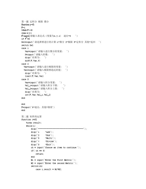
第一题定积分极限微分function y=f1F=1while F~=0syms x y zF=input('请输入表达式:(变量为x,y,z) 退出-0 ')if F~=0Sel=input('请选择要进行的计算:1-微分 2-极限 3-定积分其他-返回 ') switch Selcase 1Var=input('请输入进行微分的变量: ')N=input('请输入阶数: ')disp('结果为: ')diff(F,Var,N)case 2Var=input('请输入进行极限的变量: ')Val=input('请输入极限要趋近的值: ')disp('结果为: ')limit(F,Var,Val)case 3Var=input('请输入积分变量: ')Val_1=input('请输入积分下限: ')Val_2=input('请输入积分上限: ')disp('结果为: ')int(F,Var,Val_1,Val_2)endendF=input('0-退出,其他-继续')end第二题矩阵的运算function y=f2%syms result;while(1)disp('--------------------------------------');disp('1 -Add');disp('2 -Sub');disp('3 -Multi');disp('4 -Divide');disp('0 -Exit');ch = input('Choose an item to continue:');if( ch == 0)return;endM1 = input('Enter the first Matrix:');M2 = input('Enter the second Matrix:');switch(ch)case 1,result = M1+M2;case 2,result = M1-M2;case 3,result = M1*M2;case 4,result = M1/M2;enddisp('The result is :');disp(result);end%End function第三题矩阵的操作function y=f3while(1)disp('--------------------------------------');disp('1 -转置');disp('2 -求秩');disp('3 -求逆');disp('4 -行列式');disp('0 -Exit');ch = input('Choose an item to continue:');if( ch == 0)return;endM = input('Enter the Matrix:');switch(ch)case 1,result = M';case 2,result = rank(M);case 3,result = inv(M);case 4,result = det(M);enddisp('The transform result is :');disp(result);end%End functionendendend第四题向量的判定function y=f4(vec_1,vec_2,dem_1)vec_1=input('第一个向量:')vec_2=input('第二个向量:')Sel_2=input('选择: 1-判断两向量是否共线 2-判断三向量是否共面') if Sel_2==1A=[vec_1;vec_2]if rank(A)==1disp('两向量共线!')elsedisp('两向量不共线!')endelse if Sel_2==2vec_3=input('请输入第三个向量:')dem_3=length(vec_3)if dem_3==dem_1if cro(vec_1,vec_2)*vec_3'==0disp('三向量共面!')elsedisp('三向量不共面!')endelsedisp('输入向量维数不一致!')endendend第五题向量的长度,方向角的计算点积叉积混合积及投影的计算function y=f5n=1while n~=0vec_1=input('请输入第一个向量:')dem_1=length(vec_1)Sel=input('请选择:1-计算向量的方向角,长度 2-计算向量其他运算其他-返回')if Sel==2vec_2=input('请输入第二个向量:')dem_2=length(vec_2)if dem_1==dem_2Sel_1=input('请选择运算:1-点积 2-向量积(三维) 3-投影(三维) 4-混合积(三维) 5-判断共线,共面')switch Sel_1case 5JUDGE(vec_1,vec_2,dem_1)case 1vec_1*vec_2'case 2PAN(vec_1,vec_2)case 3vec_1*vec_2'./sqrt(vec_2*vec_2')case 4vec_3=input('请输入第三个向量(三维):')dem_3=length(vec_3)if dem_3==dem_1A=PAN(vec_1,vec_2)*vec_3'else disp('维数不一致!')endendelsedisp('输入错误!')endelseif Sel==1disp('模为:')Mol=sqrt(vec_1*vec_1')A=eye(dem_1)m=1while m~=dem_1+1acos(A(m,:)*vec_1'./(sqrt(A(m,:)*A(m,:)')*Mol))*180/pim=m+1endelsen=0endendSel=input('继续计算向量的长度、方向角的计算','向量的点积、叉积、混合积及投影-1,退出-2: ')if Sel==2n=0endend第六题点到直线,平面的距离的计算function y=f6n=1while n~=0Point=input('请输入一个三维点坐标向量:')Sel=input('请选择: 1-点到直线的距离 2-点到面的距离 ')switch Selcase 1LinVec=input('请输入直线方程的方向向量:(三维)')LinPot=input('请输入直线方程所经过的点:(三维)')if length(LinVec)==length(LinPot) & length(LinVec)==length(Point)A=p(LinVec,LinPot-Point)disp('点到直线的距离为:')A*A'./(LinVec*LinVec')else disp('输入数值是非法数值!确认后请重新输入!')endPoint=input('1-继续 2-退出')if Point==2n=0endcase 2PlantVec=input('请输入平面法向量:')PlantPot=input('请输入平面上任意一点:')if length(PlantVec)==length(PlantPot) & length(PlantVec)==length(Point)disp('点到平面的距离为:')[PlantPot-Point]*PlantVec'./(PlantVec*PlantVec')disp('输入数值是非法数值!确认后请重新输入!') end endend第七题 椭圆球 function y=pic1 a = 10; b = 20; c = 10;[x,y] = meshgrid(-2:0.1:2,-2:0.1:2);xa = x.^2/a^2; yb = y.^2/b^2;xyz = (ones(size(x))-xa-yb)*c^2; z = xyz.^0.5; mesh(x,y,z);第八题 双曲抛物面 function []=pic2 a = 5; b = 5;[x,y] = meshgrid(-2:0.1:2,-2:0.1:2);xa = x.^2/a^2; yb = y.^2/b^2; z = yb-xa; mesh(x,y,z);第九题 椭圆抛物面 function y=pic3 a = 2; b = 2;[x,y] = meshgrid(-2:0.1:2,-2:0.1:2);xa = x.^2/a^2; yb = y.^2/b^2; z = xa+yb; mesh(x,y,z);第十题 单页双曲面 function y=pic4 theta=0:pi/20:2*pi rho=1:0.05:3[theta,rho]=meshgrid(theta,rho) r=sqrt(rho.^2-1)[x,y,z]=pol2cart(theta,rho,r)figure(1)hold on z=-zsurf(x,y,z) axis off第十一题 双叶双曲面 function k=pic5t1=[-2*pi:0.05:2*pi]; t2=[-1*pi:0.05:1*pi];[t1,t2]=meshgrid(-2*pi:0.05:2*pi,-1*pi:0.05:1*pi); z=0.2*sqrt(sin(t2).*sin(t2)+1);h1=mesh(2*cos(t1).*sin(t2),sin(t1).*sin(t2),z);hold onh2=mesh(2*cos(t1).*sin(t2),sin(t1).*sin(t2),-z);第十二题椭圆锥面function k=tupian4(x,y)x=[-3:0.01:3];y=[-2:0.01:2];[x,y]=meshgrid(-3:0.01:3,-2:0.01:2); z=sqrt((x/3).^2+(y/2).^2); mesh(x,y,z); hold onmesh(x,y,-z);第十三题 常见二维图形theta=0:0.1:2*pi figure(1) rho=2*thetapolar(theta,rho) title('r=at')t=-2*pi:0.1:2*pi figure(1)x=2*(t-sin(t)) y=2*(1-cos(t)) plot(x,y,'g') xlabel('x') ylabel('y') title('摆线')theta=0:0.1:10*pi figure(1)rho=sqrt(4*sin(2*theta)) polar(theta,rho,'g') hold on rho=-rhopolar(theta,rho,'g')legend('r^2=a^2sin2t',2) hold onrho=sqrt(4*cos(2*theta)) polar(theta,rho,'r') hold on rho=-rhopolar(theta,rho,'r')legend('r^2=a^2cos2t',2)theta=0:0.1:4*pi figure(1)rho=exp(0.2*theta) polar(theta,rho) title('r=exp(at)')x=-5:0.1:5y=(1/sqrt((2*pi)))*exp(-x.^2./2) figure(1)plot(x,y,'g') xlabel('x') ylabel('y')title('概率曲线 ')t=0:0.1:2*pi figure(1)x=2*(cos(t)).^3 y=2*(sin(t)).^3 plot(x,y,'g') xlabel('x') ylabel('y')title('x^2/3+y^2/3=a^2/3')theta=0:0.1:2*pi figure(1)rho=2*cos(3*theta) polar(theta,rho,'g')legend('r=asin3t',4)hold onrho=2*sin(3*theta) polar(theta,rho,'r')legend('r=acos3t')theta=0:0.1:2*pi figure(1)rho=2*cos(2*theta) polar(theta,rho,'g') legend('r=acos2t',4)t=0:0.1:2*pi figure(1) x=2*cos(t) y=2*sin(t) plot(x,y,'g') xlabel('x') ylabel('y')title('x^2/a^2+y^2/b^2=1')theta=0:0.1:2*pi figure(1)rho=2*(1-cos(theta)) polar(theta,rho)title('r=a(1-cos(t))')x=-1:(1/20):1 figure(1)subplot(2,2,1) y=asin(x)plot(x,y,'g') title('asin(x)') axis([-1 1 -2 2])subplot(2,2,2) y=acos(x)plot(x,y,'g') title('acos(x)') axis([-1 1 0 4])subplot(2,2,3)y=atan(x)plot(x,y,'g') title('atan(x)') hold on y=y+piplot(x,y,'--') hold on y=y-2*piplot(x,y,'--')axis([-1.5 1.5 -4 4])subplot(2,2,4) y=atan(x)plot(x,y,'g') title('acot(x)') x=-xy=y+pi/2plot(x,y,'--') hold on y=y+piplot(x,y,'--') hold on y=y-2*piplot(x,y,'--')axis([-1.5 1.5 -pi 2*pi])x=-5:0.1:5y=8*2.^3./(x.^2+4*2.^2) figure(1)plot(x,y,'g') hold on x=-2:0.1:2y=sqrt(4-x.^2)+2 plot(x,y,'r') hold ony=-sqrt(4-x.^2)+2 plot(x,y,'r')xlabel('x') ylabel('y')title('y=8a^3/(x^2+4a^2)')y=-5:0.1:5 figure(1)x=(2*(1+y.^2)).^(0.5)plot(x,y,'g')hold onx=-xplot(x,y,'g') xlabel('x') ylabel('y')title('x^2/a^2-y^2/b^2=1')x=-2:0.1:2 figure(1)subplot(2,4,1) y=x.^2plot(x,y,'g') title('x^2')subplot(2,4,2) y=x.^3plot(x,y,'g') title('x^3')subplot(2,4,3) y=x.^(-1)plot(x,y,'g') title('1/x')subplot(2,4,4) x=0:0.1:2 y=x.^0.5plot(x,y,'g')title('x^(1/2)') subplot(2,4,5) x=-2:0.1:2y=(x.^2).^(1/3) plot(x,y,'g') title('x^(2/3)')subplot(2,4,6) x=0:0.1:2 y=x.^(1/3) plot(x,y,'g') hold on x=-x y=-yplot(x,y,'g') title('x^(1/3)')subplot(2,4,7)x=0:0.1:2plot(x,y,'g')hold ony=-yplot(x,y,'g')title('x^(1/3)')x=-4*pi:(pi/20):4*pifigure(1)subplot(2,2,1)y=sin(x)plot(x,y,'g')title('sin(x)')subplot(2,2,2)y=cos(x)plot(x,y,'g')title('cos(x)')subplot(2,2,3)x=-(pi/2-0.0001):pi/20:(pi/2-0.0001)y=tan(x)plot(x,y,'g')title('tan(x)')hold onx=x+piplot(x,y,'g')hold onx=x-2*piplot(x,y,'g')axis([-(1.5*pi-0.0001) (1.5*pi-0.0001) -10 10])subplot(2,2,4)x=0:pi/20:(pi-0.0001)y=cot(x)plot(x,y,'g')title('cot(x)')hold onx=x-piplot(x,y,'g')axis([-(pi-0.0001) (pi-0.0001) -10 10])theta=0:0.1:4*pifigure(1)polar(theta,rho) title('rt=a')。
matlab边缘检测代码
MATLAB边缘检测代码边缘检测是图像处理中常用的技术,用于识别图像中物体的轮廓。
在MATLAB中,我们可以使用不同的方法进行边缘检测,例如Sobel算子、Canny算子等。
本文将介绍MATLAB中常用的边缘检测方法,并给出相应的代码示例。
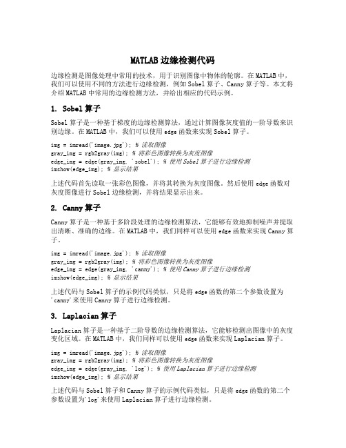
1. Sobel算子Sobel算子是一种基于梯度的边缘检测算法,通过计算图像灰度值的一阶导数来识别边缘。
在MATLAB中,我们可以使用edge函数来实现Sobel算子。
img = imread('image.jpg'); % 读取图像gray_img = rgb2gray(img); % 将彩色图像转换为灰度图像edge_img = edge(gray_img, 'sobel'); % 使用Sobel算子进行边缘检测imshow(edge_img); % 显示结果上述代码首先读取一张彩色图像,并将其转换为灰度图像。
然后使用edge函数对灰度图像进行Sobel边缘检测,并将结果显示出来。
2. Canny算子Canny算子是一种基于多阶段处理的边缘检测算法,它能够有效地抑制噪声并提取出清晰、准确的边缘。
在MATLAB中,我们同样可以使用edge函数来实现Canny算子。
img = imread('image.jpg'); % 读取图像gray_img = rgb2gray(img); % 将彩色图像转换为灰度图像edge_img = edge(gray_img, 'canny'); % 使用Canny算子进行边缘检测imshow(edge_img); % 显示结果上述代码与Sobel算子的示例代码类似,只是将edge函数的第二个参数设置为'canny'来使用Canny算子进行边缘检测。
3. Laplacian算子Laplacian算子是一种基于二阶导数的边缘检测算法,它能够检测出图像中的灰度变化区域。
matlab使用freesurfer代码

文章标题:从入门到精通:探索Matlab使用Freesurfer代码的全面指南一、Matlab及Freesurfer简介Matlab是一种强大的科学计算软件,被广泛用于工程、科学和计算领域。
而Freesurfer是一种用于大脑皮层分析的开源软件包,可用于处理结构磁共振成像(MRI)数据。
二、Freesurfer代码实现流程1. 数据准备:准备MRI数据,并使用Freesurfer进行数据预处理,包括重建、配准和分割。
2. Matlab环境配置:配置Matlab环境,确保可以调用Freesurfer 相关的函数和工具。
3. 代码编写:使用Matlab编写代码,调用Freesurfer的相关函数,实现数据处理、分析和可视化。
4. 结果展示:将处理后的结果进行可视化展示,并对结果进行分析和解释。
三、深入理解Freesurfer代码在Matlab中的应用在使用Freesurfer代码的过程中,我们需要深入理解Freesurfer的算法原理和各项函数的作用,以便能够在Matlab中灵活应用。
我们也需要熟悉Matlab的编程语法和调试技巧,以便能够高效地编写和调试Freesurfer相关的代码。
四、个人观点和建议作为一个Matlab使用者,我认为掌握Freesurfer代码在Matlab中的应用是非常有价值的。
这不仅可以帮助我们更好地理解和应用Freesurfer软件包,还可以拓展Matlab在神经影像学研究中的应用领域。
我建议在学习Matlab的也要深入学习Freesurfer软件包,并尝试在Matlab环境下进行相关代码的编写和调试。
五、总结与展望通过本文的介绍,我们对Matlab使用Freesurfer代码有了更深入的了解。
未来,希望能够进一步拓展Freesurfer在Matlab中的应用,为脑科学研究提供更多可能性和机会。
本篇文章从多个角度全面探讨了Matlab使用Freesurfer代码的相关内容,并对深度和广度要求进行了全面评估。
大学生身体素质数据的FCM算法聚类及MATLAB实现

o b j e c t o f c l a s s i i f c a i t o n n u mb e r i n c r e a s e s a n d i n c r e a s e s e x p o n e n t i a l l y , s h o u l d n o t b e a p p l i e d t o p r o mo t e . S o , w e i n r t o d u c t i o n o f
聚类特征 量 , 对大学生身 体素质进 行模糊 聚类 分析 , 利用 X i e — B e n i 有效 性指标 确定最佳 的分类方 式 , 并 利用 MA T L A B软件编程辅助计算 . 实践证 明 , 该方法操作简便 , 科学有效 , 便于应用推广 。 关键词 : 大学生 ; 身体 素质 ; 模 糊聚类分析 ; F C M 算法
Ab s t r a c t : Ac c u r a t e c l a s s i i f c a t i o n o f c o l l e g e s t u d e n t s ’ p h y s i c a l q u li a y t i s d i r e c l t y r e l a t e d t o c o l l e g e s p o r t s g r o u p t e a c h i n g , p e r s o n n e l s e l e c t i o n , e v a l u a t i o n o f t h e r a t i o n li a t y a n d e f e c t i v e n e s s . T h e t r a d i t i o n l a f u z z y c l u s t e i r n g a n ly a s i s i s t r a n s i t i v e c l o s u r e
mean-shift算法matlab代码
一、介绍Mean-shift算法Mean-shift算法是一种基于密度估计的非参数聚类算法,它可以根据数据点的密度分布自动寻找最优的聚类中心。
该算法最早由Dorin Comaniciu和Peter Meer在1999年提出,并被广泛应用于图像分割、目标跟踪等领域。
其原理是通过不断地将数据点向局部密度最大的方向移动,直到达到局部密度的最大值点,即收敛到聚类中心。
二、 Mean-shift算法的优势1. 无需事先确定聚类数量:Mean-shift算法不需要事先确定聚类数量,能够根据数据点的密度自动确定聚类数量。
2. 对初始值不敏感:Mean-shift算法对初始值不敏感,能够自动找到全局最优的聚类中心。
3. 适用于高维数据:Mean-shift算法在高维数据中仍然能够有效地进行聚类。
三、 Mean-shift算法的实现步骤1. 初始化:选择每个数据点作为初始的聚类中心。
2. 计算密度:对于每个数据点,计算其密度,并将其向密度增加的方向移动。
3. 更新聚类中心:不断重复步骤2,直至收敛到局部密度的最大值点,得到最终的聚类中心。
四、 Mean-shift算法的Matlab代码实现以下是一个简单的Matlab代码实现Mean-shift算法的示例:```matlab数据初始化X = randn(500, 2); 生成500个二维随机数据点Mean-shift算法bandwidth = 1; 设置带宽参数ms = MeanShift(X, bandwidth); 初始化Mean-shift对象[clustCent, memberships] = ms.cluster(); 执行聚类聚类结果可视化figure;scatter(X(:,1), X(:,2), 10, memberships, 'filled');hold on;plot(clustCent(:,1), clustCent(:,2), 'kx', 'MarkerSize',15,'LineWidth',3);title('Mean-shift聚类结果');```在代码中,我们首先初始化500个二维随机数据点X,然后设置带宽参数并初始化Mean-shift对象。
- 1、下载文档前请自行甄别文档内容的完整性,平台不提供额外的编辑、内容补充、找答案等附加服务。
- 2、"仅部分预览"的文档,不可在线预览部分如存在完整性等问题,可反馈申请退款(可完整预览的文档不适用该条件!)。
- 3、如文档侵犯您的权益,请联系客服反馈,我们会尽快为您处理(人工客服工作时间:9:00-18:30)。
FCM图像分割算法function fcmapp(file, cluster_n)% FCMAPP% fcmapp(file, cluter_n) segments a image named file using the algorithm% FCM.% [in]% file: the path of the image to be clustered.% cluster_n: the number of cluster for FCM.eval(['info=imfinfo(''',file, ''');']);switch info.ColorTypecase 'truecolor'eval(['RGB=imread(''',file, ''');']);% [X, map] = rgb2ind(RGB, 256);I = rgb2gray(RGB);clear RGB;case 'indexed'eval(['[X, map]=imread(''',file, ''');']);I = ind2gray(X, map);clear X;case 'grayscale'eval(['I=imread(''',file, ''');']);end;I = im2double(I);filename = file(1 : find(file=='.')-1);data = reshape(I, numel(I), 1);tic[center, U, obj_fcn]=fcm(data, cluster_n);elapsedtime = toc;%eval(['save(', filename, int2str(cluster_n),'.mat'', ''center'', ''U'', ''obj_fcn'', ''elapsedtime'');']); fprintf('elapsedtime = %d', elapsedtime);maxU=max(U);temp = sort(center, 'ascend');for n = 1:cluster_n;eval(['cluster',int2str(n), '_index = find(U(', int2str(n), ',:) == maxU);']);index = find(temp == center(n));switch indexcase 1color_class = 0;case cluster_ncolor_class = 255;otherwisecolor_class = fix(255*(index-1)/(cluster_n-1));endeval(['I(cluster',int2str(n), '_index(:))=', int2str(color_class),';']);end;filename = file(1:find(file=='.')-1);I = mat2gray(I);%eval(['imwrite(I,', filename,'_seg', int2str(cluster_n), '.bmp'');']);imwrite(I, 'temp\tu2_4.bmp','bmp');imview(I);function fcmapp(file, cluster_n)% FCMAPP% fcmapp(file, cluter_n) segments a image named file using the algorithm% FCM.% [in]% file: the path of the image to be clustered.% cluster_n: the number of cluster for FCM.eval(['info=imfinfo(''',file, ''');']);switch info.ColorTypecase 'truecolor'eval(['RGB=imread(''',file, ''');']);% [X, map] = rgb2ind(RGB, 256);I = rgb2gray(RGB);clear RGB;case 'indexed'eval(['[X, map]=imread(''',file, ''');']);I = ind2gray(X, map);clear X;case 'grayscale'eval(['I=imread(''',file, ''');']);end;I = im2double(I);filename = file(1 : find(file=='.')-1);data = reshape(I, numel(I), 1);tic[center, U, obj_fcn]=fcm(data, cluster_n);elapsedtime = toc;%eval(['save(', filename, int2str(cluster_n),'.mat'', ''center'', ''U'', ''obj_fcn'', ''elapsedtime'');']); fprintf('elapsedtime = %d', elapsedtime);maxU=max(U);temp = sort(center, 'ascend');for n = 1:cluster_n;eval(['cluster',int2str(n), '_index = find(U(', int2str(n), ',:) == maxU);']);index = find(temp == center(n));switch indexcase 1color_class = 0;case cluster_ncolor_class = 255;otherwisecolor_class = fix(255*(index-1)/(cluster_n-1));endeval(['I(cluster',int2str(n), '_index(:))=', int2str(color_class),';']); end;filename = file(1:find(file=='.')-1);I = mat2gray(I);%eval(['imwrite(I,', filename,'_seg', int2str(cluster_n), '.bmp'');']); imwrite(I, 'r.bmp');imview(I);主程序1ImageDir='.\';%directory containing the images%path('..') ;%cmpviapath('..') ;img=im2double(imresize(imread([ImageDir '12.png']),2)) ;figure(1) ; imagesc(img) ; axis image[ny,nx,nc]=size(img) ;imgc=applycform(img,makecform('srgb2lab')) ;d=reshape(imgc(:,:,2:3),ny*nx,2) ;d(:,1)=d(:,1)/max(d(:,1)) ; d(:,2)=d(:,2)/max(d(:,2)) ;%d=d ./ (repmat(sqrt(sum(d.^2,2)),1,3)+eps()) ;k=4 ; % number of clusters%[l0 c] = kmeans(d, k,'Display','iter','Maxiter',100);[l0 c] = kmeans(d, k,'Maxiter',100);l0=reshape(l0,ny,nx) ;figure(2) ; imagesc(l0) ; axis image ;%c=[ 0.37 0.37 0.37 ; 0.77 0.73 0.66 ; 0.64 0.77 0.41 ; 0.81 0.76 0.58 ; ...%0.85 0.81 0.73 ] ;%c=[0.99 0.76 0.15 ; 0.55 0.56 0.15 ] ;%c=[ 0.64 0.64 0.67 ; 0.27 0.45 0.14 ] ;%c=c ./ (repmat(sqrt(sum(c.^2,2)),1,3)+eps()) ;% Data termDc=zeros(ny,nx,k) ;for i=1:k,dif=d-repmat(c(i,:),ny*nx,1) ;Dc(:,:,i)= reshape(sum(dif.^2,2),ny,nx) ;end ;% Smoothness termSc=(ones(k)-eye(k)) ;% Edge termsg = fspecial('gauss', [13 13], 2);dy = fspecial('sobel');vf = conv2(g, dy, 'valid');Vc = zeros(ny,nx);Hc = Vc;for b=1:nc,Vc = max(Vc, abs(imfilter(img(:,:,b), vf, 'symmetric')));Hc = max(Hc, abs(imfilter(img(:,:,b), vf', 'symmetric'))); endgch=char;gch = GraphCut('open', 1*Dc, Sc,exp(-5*Vc),exp(-5*Hc)); [gch l] = GraphCut('expand',gch);gch = GraphCut('close', gch);label=l(100,200) ;lb=(l==label) ;lb=imdilate(lb,strel('disk',1))-lb ;figure(3) ; image(img) ; axis image ; hold on ;contour(lb,[1 1],'r') ; hold off ; title('no edges') ;figure(4) ; imagesc(l) ; axis image ; title('no edges') ;gch = GraphCut('open', Dc, 5*Sc,exp(-10*Vc),exp(-10*Hc)); [gch l] = GraphCut('expand',gch);gch = GraphCut('close', gch);lb=(l==label) ;lb=imdilate(lb,strel('disk',1))-lb ;figure(5) ; image(img) ; axis image ; hold on ;contour(lb,[1 1],'r') ; hold off ; title('edges') ;figure(6) ; imagesc(l) ; axis image ; title('edges') ;主程序2I = imread( '12.png' );I = rgb2gray(I);subplot(5,3,1),imshow(I);k=medfilt2(I,[5,5]);subplot(5,3,2),imshow(k);title('5*5中值滤波图像');%f=imread('tuxiang1.tif');%subplot(1,2,1),imshow(f);%title('原图像');g1=histeq(k,256);subplot(5,3,3),imshow(g1);title('直方图匹配');%g2=histeq(k2,256);%subplot(2,2,2),imshow(g2);%title('5*5直方图匹配');%k=medfilt2(f,[5,5]);%k2=medfilt2(f,[5,5]);%j=imnoise(f,'gaussian',0,0.005);%subplot(1,3,3),imshow(k2);%title('5*5中值滤波图像');hy = fspecial( 'sobel' );hx = hy;Iy = imfilter(double(g1), hy, 'replicate' );Ix = imfilter(double(g1), hx, 'replicate' );gradmag = sqrt(Ix.^2 + Iy.^2);subplot(5,3,4), imshow(gradmag,[ ]), title( 'gradmag' );L = watershed(gradmag);Lrgb = label2rgb(L);subplot(5,3,5), imshow(Lrgb), title( 'Lrgb' );se = strel( 'disk' , 9);Io = imopen(g1, se);subplot(5,3,6), imshow(Io), title( 'Io' )Ie = imerode(g1, se);Iobr = imreconstruct(Ie, g1);subplot(5,3,7), imshow(Iobr), title( 'Iobr' );Ioc = imclose(Io, se);subplot(5,3,8), imshow(Ioc), title( 'Ioc' );Iobrd = imdilate(Iobr, se);Iobrcbr = imreconstruct(imcomplement(Iobrd), imcomplement(Iobr)); Iobrcbr = imcomplement(Iobrcbr);subplot(5,3,9), imshow(Iobrcbr), title( 'Iobrcbr' );fgm = imregionalmax(Iobrcbr);subplot(5,3,10), imshow(fgm), title( 'fgm' );I2 = g1; I2(fgm) = 255;subplot(5,3,11),imshow(I2), title( 'fgm superimposed on original image' );se2 = strel(ones(5,5)); I3 = g1; I3(fgm) = 255;subplot(5,3,12) ,imshow(I3);title( 'fgm4 superimposed on original image' );bw = im2bw(Iobrcbr, graythresh(Iobrcbr));subplot(5,3,13) , imshow(bw), title( 'bw' );D = bwdist(bw); DL = watershed(D);bgm = DL == 0;subplot(5,3,14) , imshow(bgm), title( 'bgm' );gradmag2 = imimposemin(gradmag, bgm | fgm);L = watershed(gradmag2);I4 = g1;I4(imdilate(L == 0, ones(3, 3)) | bgm | fgm) = 255;figure, imshow(I4);title( 'Markers and object boundaries superimposed on original image' ); Lrgb = label2rgb(L, 'jet' , 'w' , 'shuffle' );figure, imshow(Lrgb);title( 'Lrgb' );figure, imshow(I), hold onhimage = imshow(Lrgb);set(himage, 'AlphaData' , 0.3);title( 'Lrgb superimposed transparently on original image' );。