Nonminimal Inflation and the Running Spectral Index
非线性动力学入门-西安交通大学教师个人主页

. . . . . . . .
. . . . . . . .
. . . . . . . .
. . . . . . . .
. . . . . . . .
. . . . . . . .
. . . . . . . .
. . . . . . . .
. . . . . . . .
. . . . . . . .
. . . . . . . .
. . . . . . . .
. . . . . . . .
. . . . . . . .
. . . . . . . .
. . . . . . . .
. . . . . . . . . . . . . . . . .
. . . . . . . . . . . . . . . . .
. . . . . . . . . . . . . . . . .
. . . . . . . . . . . . . . . . .
. . . . . . . . . . . . . . . . .
. . . . . . . . . . . . . . . . .
. . . . . . . . . . . . . . . . .
另一方面梁的轴向应变的表达式也会因变形大小的不同而采用不同的表达式比如小变形时应变而当考虑大变形时可能采用的应变表达式就是进而得到的梁的振动方程将会是一个含有高度非线性项的偏微分方程组
非线性动力学入门
张新华
西安交通大学 工程力学系 2011 年 07 月
前 言
─1687 年,牛顿(Isaac Newton, 1643 ~ 1727)发表了《自然哲学之数学原 理》(Mathematical Principles of Natural Philosophy),标志着经典力学(亦即牛 顿力学)的正式诞生。牛顿力学主要研究自由质点系的宏观运动规律。 ─1788 年,拉格朗日(Joseph Louis Lagrange, 1736 ~ 1813)发表了分析力 学教程(Analytical Mechanics),标志着拉格朗日力学的诞生。Lagrange 力学属 于分析力学的主要内容之一,在位形空间中研究带有约束的质点系动力学。 ─1833 年,哈密尔顿(William Rowen Hamilton, 1805 ~ 1865)对 Lagrange 力学进行了改造,引进了相空间(2n 维空间),对系统内在的对称性(辛对称, Symplectic)进行了刻画。狭义上的哈密尔顿力学只适用于保守系统,而广义 的哈密尔顿力学在适用于非保守系统。哈密尔顿力学也属于分析力学的主要 组成部分。在此后发展起来的量子力学中 Hamilton 力学发挥着巨大的作用。 目前在天体力学、计算 Hamilton 力学,量子力学,甚至弹性力学(即所谓的 辛弹性力学)中哈密尔顿力学依然发挥着重要作用。 ─1927 年,Birkhoff(George David Birkhoff, 1844 ~ 1944)发表了“动力系 统”(Dynamical Systems),标志着 Birkhoff 动力学的正式问世。Birkhoff 动力 学建立了研究非完整力学的框架。 ─1892 ~ 1899, 彭加莱(Henri Poincaré, 1854 ~ 1912)发表了三卷本的“天 体力学中的新方法”(New Methods of Celestial Mechanics),系统性地提出了 研究动力学系统的定性方法,即几何方法。经典力学的目标之一就是设法求 得系统的解析解,而 Poincaré意识到对于大多数非线性系统而言,求其解析 解是不可能的,而必须发展新的研究方法。他超越了他的时代,极富远见地 预测到了非线性系统混沌现象(系统的解对初始条件具有极端敏感依赖性)的 存在。更为重要的是,Poincaré开创了研究非线性动力系统的几何方法,当之 无愧地被誉为非线性科学之父,其影响是划时代的。 ─1892 年,李亚普诺夫(Aleksandr Mikhailovich Lyapunov, 1857 ~ 1918)在 他的博士论文“运动稳定性的一般问题”(General problem of the stability of motion )中,系统地探讨了非线性动力学系统的稳定性问题。他提出了两种研 究稳定性的方法:李亚普诺夫第一方法(间接方法)和李亚普诺夫第二方法(直 接方法)。他从代数角度出发,对动力学系统的研究开创了一个崭新的领域。 彭加莱与李亚普诺夫,前者从几何角度,后者从代数角度,开拓了非线 性科学的研究疆域和研究手段。 ─1963 年,Lorenz(Edward Norton Lorenz, 1917 ~ 2008)发表了“确定性 非周期流”(Deterministic Nonperiodic Flow)的论文,认为大气系统的性态对 初值极为敏感,从而导致准确的长期天气预报是不可能的。该文标志着人类 首次借助于计算机发现了混沌(Chaos)现象的存在。 ─1757 年,欧拉(Leonhard Euler, 1707 ~ 1783)发表了压杆稳定性的论 文,首次探讨了力学系统的分岔现象。作为分岔理论重要分支的突变理 论(Catastrophe Theory)则主要由法国数学家托姆(René Thom, 1923 ~ 2002)于 上个世纪 60 年代创立,由齐曼(Christopher Zeeman,1925 ~)在 70 年代大力 推广普及。 ─1834 年,英国的罗素(John Scott Russell, 1808 ~ 1882)骑着马在 Union 运河上散步时,发现了现在称之为孤立波(又称作孤波,Solitary wave)的 i
物理海洋学期末复习资料
代替。
第五章
1.梯度流、倾斜流的表达式(������������������������)
A.海流是海洋中发生的一种有相对稳定速度的大规模的非周期性流动。 其发生的原因有两种:a.受海面风力的作用(动力学);b.海面受热冷却不均匀、蒸发降水不均匀所产生的温 度、盐度从而引起密度分布不均匀(热力学)。
M:融冰 ������������:海流及混合使海域失去的水量
第四章
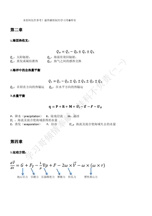
1.运动方程:
���������⃗��� ������������
=
������
+
������������
−
1 ������
∇������
+
������
−
2������
×
���⃗ ���
−
������
×
(������
×
������)
A.建立了一个考虑海底摩擦效应,封闭的矩形大洋中的漂流模式,即考虑西边界区域;
B.结果指出 f 随维度变化,即β效应是产生海流西向强化的基本原因。
(4)Munk 理论
A.整个大洋环流呈现西部强化现象
①以纬度向为主
②都随着 x 增大而衰减
B.大洋西边界质量输运特点:
③在西边界区域有一强烈的北向流动,近岸处质量运输很大,随着离岸距
3.风生大洋环流的几个理论成果(������������������������)
(1)边界层技术:作为整个大洋,其中的运动应该有个统一解。这个统一解是一个衔接方法,它将边界层内的 解与大洋内部区域的解,适当衔接起来,组成一个大洋环流解。重要的问题是选择合适的、具有边界层厚度的长 度尺度。按这个尺度去简化边界层内的方程,使解相对容易求得并满足边界条件。而当把边界层坐标系延长时,
d维RN-AdS黑洞的弱宇宙审查猜想

Applications 创新应用集成电路应用 第 39 卷 第 4 期(总第 343 期)2022 年 4 月 69们认为奇点是密度无穷大的一个点,在这个点附近一切物理定律都无法使用,这与我们目前已知的情况格格不入,即是说明我们目前已知的物理规律、量子力学、场论等等一切物理规律都是无效的在奇点附近。
为了保证已知的物理定律的真实性和有效性,1969年彭罗斯从类时测地线受到启发提出了弱宇宙审查猜想来保证物理规律可行性,他的猜想表明黑洞坍塌诞生的奇点应该被黑洞视界包着,视界在奇点的外围,奇点被视界隐藏在后面,远处的研究人员不能通过任何方法无法得到奇点附近的任何信息。
由于对于奇点附近的问题一直得不到解决,而人们又急需一种理论来说明这种情况,于是很多学者开始赞同彭罗斯宇宙审查猜想,用事件视界来隔离奇点内外情况,用事件视界作为边界,视界内部是奇点所在时空,外界对其不会有任何影响,视界外部的一切也不会影响到视界内部,虽然这种说法能暂时将奇点问题屏蔽,但是其说法很难得到广大科学家认同。
自从彭罗斯最初的研究结果以来,弱宇宙审查猜想(WCCC)一直是黑洞的一个有趣的研0 引言拉普拉斯(Laplace)和米谢尔(Michelle)通过对天体研究发现,存在一类天体其第二宇宙速度超过光速,我们无法观测到它,因为一切靠近它的物质包括光都会被其巨大的引力拖拽,人们把这种天体称为暗星[1]。
1 研究背景100多年后爱因斯坦在1915年提出相对论,他认为质量的存在会影响周围的时空,使周围时空发生弯曲,如果一个天体质量足够大,其产生的弯曲曲率能使光线都发生偏折,并向中心天体靠近,那么光进入之后就无法出来,之后史瓦西通过对场方程求解得到了一个真空球对称解——史瓦西解,美国科学家惠勒将这种天体现象称为黑洞(BH)。
之后人们对黑洞性质,及其满足的物理规律都有极大兴趣,在1960~1970年代,霍金和彭罗斯对黑洞的形成进行研究,他们发现只有相对论有效,满足因果性,黑洞内部就一定是奇异的。
南中国海内波特征及其引起的声场起伏.pdf
图!
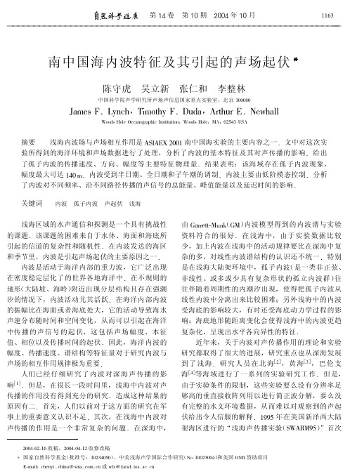
"#$"%& ’((! 实验海域及主要实验设备布放图
( +)实验海域及设备; (0) 海水温度剖面; ( 2) 海水盐度剖面; (3) 声速剖面; ( 1)浮力频率剖面
’ 研究思路和方法
本文主要做了两方面的工作 ! 其一,是对内波 活动规律的研究 ! 其二,是对内波引起声传播起伏 的研究 !
由实验所得的大量温度和海流数据可以直接观 察内波活动的情况 ! 除了观察内波的时空分布、幅 度、特征宽度等特征量以外,还可以利用温度链的 空间分布计算得到孤子内波的传播速度 ! 由水文数 据处理可以计算得到内波各简正波模态的空间分布
摘要
浅海内波场与声场相互作用是 7IB79Q D""! 南中国海实验的主要内容之一 * 文中对这次实
验所得到的海洋环境和声场数据进行了处理,分析了内波的基本特征及其对声传播的影响 * 给出 了孤子内波的传播速度、方向、幅度等主要特征物理量 * 结果表明:该海域存在孤子内波现象, 幅度最大可达 !F" &* 内波受到半日潮、全日潮和子午潮的调制 * 内波主要由低阶模态控制 * 分析 了内波对不同频率、沿不同路径传播的声信号的总能量、峰值能量以及延迟时间的影响 * 关键词
%%4&
第 !" 卷
第 !# 期
$##" 年 !# 月
给出了比较丰富的实验数据,检验了一些重要的理 论模型 ! 但是,此次实验侧重于对垂直于大陆架方 向的声传播的研究,对平行于大陆架方向的声传播
["] 的研究不充分 !
及水声数据进行处理,研究内波的特征参数以及内 波引起声场起伏的规律 !
!
实验简介
指向此处 !
日 6789 观测到的流的水平速度按照垂直等深线 (方 向角为 #)/() 和平行等深线 (方向角为 //() 进行分解, 见图版 (:( );) 6 ! 在大多数情况下,平行等深线方向 ! 的流速比垂直等深线方向的流速小得多,因此可以判 定不同孤子内波的传播方向大致相同 ! 但是,也有一 些时候,这两个流速的大小可以比拟,这说明孤子内 波的传播方向不尽相同,孤子内波的激发源地也可能 不尽相同 ! 对同步合成孔径雷达图象的分析表明,实 验海域南方的东沙群岛海域在 * 月 #< 日就激发出明
天文学会专业词汇【4】

Sagittarius dwarf ⼈马矮星系 Sagittarius dwarf galaxy ⼈马矮星系 Sagittarius galaxy ⼈马星系 Saha equation 沙哈⽅程 Sakigake 〈先驱〉空间探测器 Saturn-crossing asteroid 越⼟⼩⾏星 Saturnian ringlet ⼟星细环 Saturnshine ⼟星反照 scroll 卷滚 Sculptor group ⽟夫星系群 Sculptor Supercluster ⽟夫超星系团 Sculptor void ⽟夫巨洞 secondary crater 次级陨击坑 secondary resonance 次共振 secular evolution 长期演化 secular resonance 长期共振 seeing management 视宁度控管 segregation 层化 selenogony ⽉球起源学 separatrice 分界 sequential estimation 序贯估计 sequential processing 序贯处理 serendipitous X-ray source 偶遇 X 射线源 serendipitous γ-ray source 偶遇γ射线源 Serrurier truss 赛路⾥桁架 shell galaxy 壳星系 shepherd satellite 牧⽺⽝卫星 shock temperature 激波温度 silicon target vidicon 硅靶光导摄象管 single-arc method 单弧法 SIRTF, Space Infrared Telescope 空间红外望远镜 Facility slitless spectroscopy ⽆缝分光 slit spectroscopy 有缝分光 slow pulsar 慢转脉冲星 SMM, Solar Maximum MIssion 太阳极⼤使者 SMT, Submillimeter Telescope 亚毫⽶波望远镜 SOFIA, Stratospheric Observatory for 〈索菲雅〉机载红外望远镜 Infrared Astronomy soft γ-ray burst repeater 软γ暴复现源 soft γ repeater ( SGR )软γ射线复现源 SOHO, Solar and Heliospheric 〈索贺〉太阳和太阳风层探测器 Observatory solar circle 太阳圈 solar oscillation 太阳振荡 solar pulsation 太阳脉动 solar-radiation pressure 太阳辐射压 solar-terrestrial environment ⽇地环境 solitary 孤⼦性 soliton star 孤⼦星 South Galactic Cap 南银冠 South Galactic Pole 南银极 space density profile 空间密度轮廓 space geodesy 空间⼤地测量 space geodynamics 空间地球动⼒学 Spacelab 空间实验室 spatial mass segregation 空间质量分层 speckle masking 斑点掩模 speckle photometry 斑点测光 speckle spectroscopy 斑点分光 spectral comparator ⽐长仪 spectrophotometric distance 分光光度距离 spectrophotometric standard 分光光度标准星 spectroscopic period 分光周期 specular density 定向密度 spherical dwarf 椭球矮星系 spin evolution ⾃旋演化 spin period ⾃旋周期 spin phase ⾃旋相位 spiral 旋涡星系 spiral arm tracer ⽰臂天体 Spoerer minimum 斯珀勒极⼩ spotted star 富⿊⼦恒星 SST, Spectroscopic Survey Telescope 分光巡天望远镜 standard radial-velocity star 视向速度标准星 standard rotational-velocity star ⾃转速度标准星 standard velocity star 视向速度标准星 starburst 星暴 starburst galaxy 星暴星系 starburst nucleus 星暴 star complex 恒星复合体 star-formation activity 产星活动 star-formation burst 产星暴 star-formation efficiency ( SFE )产星效率 star-formation rate 产星率 star-formation region 产星区 star-forming region 产星区 starpatch 星斑 static property 静态特性 statistical orbit-determination 统计定轨理论 theory steep-spectrum radio quasar 陡谱射电类星体 stellar environment 恒星环境 stellar halo 恒星晕 stellar jet 恒星喷流 stellar speedometer 恒星视向速度仪 stellar seismology 星震学 Stokes polarimetry 斯托克斯偏振测量 strange attractor 奇异吸引体 strange star 奇异星 sub-arcsec radio astronomy 亚⾓秒射电天⽂学 Subaru Telescope 昴星望远镜 subcluster 次团 subclustering 次成团 subdwarf B star B 型亚矮星 subdwarf O star O 型亚矮星 subgiant branch 亚巨星⽀ submilliarcsecond optical astrometry 亚毫⾓秒光波天体测量 submillimeter astronomy 亚毫⽶波天⽂ submillimeter observatory 亚毫⽶波天⽂台 submillimeter photometry 亚毫⽶波测光 submillimeter space astronomy 亚毫⽶波空间天⽂ submillimeter telescope 亚毫⽶波望远镜 submillisecond optical pulsar 亚毫秒光学脉冲星 submillisecond pulsar 亚毫秒脉冲星 submillisecond radio pulsar 亚毫秒射电脉冲星 substellar object 亚恒星天体 subsynchronism 亚同步 subsynchronous rotation 亚同步⾃转 Sunflower galaxy ( M 63 )葵花星系 sungrazer comet 掠⽇彗星 supercluster 超星团; 超星系团 supergalactic streamer 超星系流状结构 supergiant molecular cloud ( SGMC )超巨分⼦云 superhump 长驼峰 superhumper 长驼峰星 supermaximum 长极⼤ supernova rate 超新星频数、超新星出现率 supernova shock 超新星激波 superoutburst 长爆发 superwind galaxy 超级风星系 supporting system ⽀承系统 surface activity 表⾯活动 surface-brightness profile ⾯亮度轮廓 surface-channel CCD 表⾯型 CCD SU Ursae Majoris star ⼤熊 SU 型星 SWAS, Submillimeter Wave Astronomy 亚毫⽶波天⽂卫星 Satallite symbiotic binary 共⽣双星 symbiotic Mira 共⽣刍藁 symbiotic nova 共⽣新星 synthetic-aperture radar 综合孔径雷达 systemic velocity 质⼼速度TAMS, terminal-age main sequence 终龄主序 Taurus molecular cloud ( TMC )⾦⽜分⼦云 TDT, terrestrial dynamical time 地球⼒学时 television guider 电视导星器 television-type detector 电视型探测器 Tenma 〈天马〉X 射线天⽂卫星 terrestrial reference system 地球参考系 tetrad 四元基 thermal background 热背景辐射 thermal background radiation 热背景辐射 thermal pulse 热脉冲 thermonuclear runaway 热核暴涨 thick-disk population 厚盘族 thinned CCD 薄型 CCD third light 第三光源 time-signal station 时号台 timing age 计时年龄 tomograph 三维结构图 toner 调⾊剂 torquetum ⾚基黄道仪 TRACE, Transition Region and Coronal 〈TRACE〉太阳过渡区和⽇冕 Explorer 探测器 tracker 跟踪器 transfer efficiency 转移效率 transition region line 过渡区谱线 trans-Nepturnian object 海外天体 Trapezium cluster 猎户四边形星团 triad 三元基 tri-dimensional spectroscopy 三维分光 triquetum 三⾓仪 tuning-fork diagram ⾳叉图 turnoff age 拐点年龄 turnoff mass 拐点质量 two-dimensional photometry ⼆维测光 two-dimensional spectroscopy ⼆维分光 UKIRT, UK Infrared Telescope Facility 联合王国红外望远镜 UKST, UK Schmidt Telescope 联合王国施密特望远镜 ultracompact H Ⅱ region 超致密电离氢区 ultradeep-field observation 特深天区观测 ultraluminous galaxy 超⾼光度星系 ultrametal-poor star 特贫⾦属星 Ulysses 〈尤利西斯〉太阳探测器 unseen component 未见⼦星 upper tangent arc 上正切晕弧 unnumbered asteroid 未编号⼩⾏星 Uranian ring 天王星环 Ursa Major group ⼤熊星群 Ursa Minorids ⼩熊流星群 Vainu Bappu Observatory 巴普天⽂台 variable-velocity star 视向速度变星 vectorial astrometry ⽮量天体测量 vector-point diagram ⽮点图 Vega 〈维佳〉⾏星际探测器 Vega phenomenon 织⼥星现象 velocity variable 视向速度变星 Venera 〈⾦星〉号⾏星际探测器 very strong-lined giant, VSL giant 甚强线巨星 very strong-lined star, VSL star 甚强线星 video astronomy 录象天⽂ viewfinder 寻星镜 Viking 〈海盗〉号⽕星探测器 virial coefficient 位⼒系数 virial equilibrium 位⼒平衡 virial radius 位⼒半径 virial temperature 位⼒温度 virtual phase CCD 虚相 CCD visible arm 可见臂 visible component 可见⼦星 visual star 光学星 VLT, Very Large Telescope 甚⼤望远镜 void 巨洞 Vondrak method 冯德拉克⽅法 Voyager 〈旅⾏者〉号⾏星际探测器 VSOP, VLBI Space Observatory 空间甚长基线⼲涉测量 Programme 天⽂台计划 wave-front sensor 波前传感器 weak-line T Tauri star 弱线⾦⽜ T 型星 Wesselink mass 韦塞林克质量 WET, Whole Earth Telescope 全球望远镜 WHT, William Herschel Telescope 〈赫歇尔〉望远镜 wide-angle eyepiece ⼴⾓⽬镜 wide binary galaxy 远距双重星系 wide visual binary 远距⽬视双星 Wild Duck cluster ( M 11 )野鸭星团 Wind 〈风〉太阳风和地球外空磁层 探测器 WIRE, Wide-field Infrared Explorer 〈WIRE〉⼴⾓红外探测器 WIYN Telescope, Wisconsin-Indiana- 〈WIYN〉望远镜 Yale-NOAO Telescope WR nebula, Wolf-Rayet nebula WR 星云 Wyoming Infrared Telescope 怀俄明红外望远镜 xenobiology 外空⽣物学 XMM, X-ray Mirror Mission X 射线成象望远镜 X-ray corona X 射线冕 X-ray eclipse X 射线⾷ X-ray halo X 射线晕 XTE, X-ray Timing Explorer X 射线计时探测器 yellow straggler 黄离散星 Yohkoh 〈阳光〉太阳探测器 young stellar object ( YSO )年轻恒星体 ZAHB, zero-age horizontal branch 零龄⽔平⽀ Zanstra temperature 赞斯特拉温度 ZZ Ceti star 鲸鱼 ZZ 型星 γ-ray burster ( GRB )γ射线暴源 γ-ray line γ谱线 γ-ray line astronomy γ谱线天⽂ γ-ray line emission γ谱线发射 ζ Aurigae binary 御夫ζ型双星 ζ Aurigae variable 御夫ζ型变星absolute energy distribution 绝对能量分布 abundance effect 丰度效应 angular diameter—redshift relation ⾓径—红移关系 asteroid astrometry ⼩⾏星天体测量 bursting pulsar ( GRO J1744-28 )暴态脉冲星 Caliban 天卫⼗七 canonical Big Bang 典型⼤爆炸 Cepheid binary 造⽗双星 CH anomaly CH 反常 chromospheric plage ⾊球谱斑 circumnuclear star-forming ring 核周产星环 circumstellar astrophysics 星周天体物理 CN anomaly CN 反常 colliding-wind binary 星风互撞双星 collisional de-excitation 碰撞去激发 collisional ionization 碰撞电离 collision line broadening 碰撞谱线致宽 Compton loss 康普顿耗损 continuous opacity 连续不透明度 coronagraphic camera ⽇冕照相机 coronal active region ⽇冕活动区 cosmic-ray exposure age 宇宙线曝射法年龄 count—magnitude relation 计数—星等关系 Cousins color system 卡曾斯颜⾊系统 dating method 纪年法 DDO color system DDO 颜⾊系统 deep sky object 深空天体 deep sky phenomena 深空天象 dense star cluster 稠密星团 diagnostics 诊断法 dissociative recombination 离解复合 Doppler line broadening 多普勒谱线致宽 epicyclic orbit 本轮轨道 extragalactic background 河外背景 extragalactic background radiation 河外背景辐射 flare particle emission 耀斑粒⼦发射 flare physics 耀斑物理 Fm star Fm 星 focal plane spectrometer 焦⾯分光计 focusing X-ray telescope 聚焦 X 射线望远镜 Friedmann time 弗⾥德曼时间 galactic chimney 星系通道 Galactic chimney 银河系通道 gas relention age ⽓体变异法年龄 Gauss line profile ⾼斯谱线轮廓 GCR ( Galactic cosmic rays )银河系宇宙线 Geneva color system ⽇内⽡颜⾊系统 global oscilletion 全球振荡 GW-Vir instability strip 室⼥ GW 不稳定带 Highly Advanced Laboratory for 〈HALCA〉通讯和天⽂⾼新空间 Communications and Astronomy 实验室 ( HALCA ) Hipparcos catalogue 依巴⾕星表 Hobby-Eberly Telescope ( HET )〈HET〉⼤型拼镶镜⾯望远镜 Hoyle—Narlikar cosmology 霍伊尔—纳⾥卡宇宙学 Hubble Deep Field ( HDF )哈勃深空区 human space flight 载⼈空间飞⾏、⼈上天 imaging spectrograph 成象摄谱仪 infrared camera 红外照相机 infrared luminosity 红外光度 infrared polarimetry 红外偏振测量 in-situ acceleration 原位加速 intercept age 截距法年龄 inverse Compton limit 逆康普顿极限 isochron age 等龄线法年龄 Johnson color system 约翰逊颜⾊系统 K giant variable ( KGV ) K 型巨变星 kinetic equilibrium 运动学平衡 large-scale beam ⼤尺度射束 large-scale jet ⼤尺度喷流 limb polarization 临边偏振 line-profile variable 谱线轮廓变星 long term fluctuation 长期起伏 Lorentz line profile 洛伦兹谱线轮廓 magnetic arm 磁臂 Mars globe ⽕星仪 massive black hole ⼤质量⿊洞 mean extinction coefficient 平均消光系数 mean luminosity density 平均光度密度 microwave storm 微波噪暴 Milli-Meter Array ( MMA )〈MMA〉毫⽶波射电望远镜阵 molecular maser 分⼦微波激射、分⼦脉泽 moving atmosphere 动态⼤⽓ neutrino loss rate 中微⼦耗损率 non-linear astronomy ⾮线性天⽂ non-standard model ⾮标准模型 passband width 带宽 P Cygni type star 天鹅 P 型星 Perseus chimney 英仙通道 planetary companion 似⾏星伴天体 plateau phase 平台阶段 primordial abundance 原始丰度 protobinary system 原双星 proto-brown dwarf 原褐矮星 quiescent galaxy 宁静星系 radiation transport 辐射转移 radio-intermediate quasar 中介射电类星体 random peculiar motion 随机本动 relative energy distribution 相对能量分布 RGU color system RGU 颜⾊系统 ringed barred galaxy 有环棒旋星系 ringed barred spiral galaxy 有环棒旋星系 rise phase 上升阶段 Rossi X-ray Timing Explorer ( RXTE )〈RXTE〉X 射线时变探测器 RQPNMLK color system RQPNMLK 颜⾊系统 Scheuer—Readhead hypothesis 朔伊尔—⾥德⿊德假说 Serpens molecular cloud 巨蛇分⼦云 soft X-ray transient ( SXT )软 X 射线暂现源 solar dynamo 太阳发电机 solar global parameter 太阳整体参数 solar neighbourhood 太阳附近空间 spectral catalogue 光谱表 spectral duplicity 光谱成双性 star-formation process 产星过程 star-forming phase 产星阶段 Stroemgren color system 颜⾊系统 Sub-Millimeter Array ( SMA )〈SMA〉亚毫⽶波射电望远镜阵 superassociation 超级星协 supermassive black hole 特⼤质量⿊洞 supersoft X-ray source 超软 X 射线源 super-star cluster 超级星团 Sycorax 天卫⼗七 symbiotic recurrent nova 共⽣再发新星 synchrotron loss 同步加速耗损 time dilation 时间扩展 tired-light model 光线⽼化宇宙模型 tremendous outburst amplitude 巨爆幅 tremendous outburst amplitude dwarf 巨爆幅矮新星 nova ( TOAD ) Tycho catalogue 第⾕星表 UBV color system UBV 颜⾊系统 UBVRI color system UBVRI 颜⾊系统 ultraviolet luminosity 紫外光度 unrestricted orbit ⽆限制性轨道 uvby color system uvby 颜⾊系统 VBLUW color system VBLUW 颜⾊系统 Venus globe ⾦星仪 Vilnius color system 维尔纽斯颜⾊系统 Virgo galaxy cluster 室⼥星系团 VLBA ( Very Long Baseline Array )〈VLBA〉甚长基线射电望远镜阵 Voigt line profile 佛克特谱线轮廓 VRI color system VRI 颜⾊系统 Walraven color system 沃尔拉⽂颜⾊系统 waning crescent 残⽉ waning gibbous 亏凸⽉ waxing crescent 娥眉⽉ waxing gibbous 盈凸⽉ WBVR color system WBVR 颜⾊系统 Wood color system 伍德颜⾊系统 zodiacal light photometry 黄道光测光 11-year solar cycle 11 年太阳周 α Cygni variable 天津四型变星 δ Doradus variable 剑鱼δ型变星。
黑洞的准正模式(quasinormal modes)

Quasi-Normal Modes of Stars and Black HolesKostas D.KokkotasDepartment of Physics,Aristotle University of Thessaloniki,Thessaloniki54006,Greece.kokkotas@astro.auth.grhttp://www.astro.auth.gr/˜kokkotasandBernd G.SchmidtMax Planck Institute for Gravitational Physics,Albert Einstein Institute,D-14476Golm,Germany.bernd@aei-potsdam.mpg.dePublished16September1999/Articles/Volume2/1999-2kokkotasLiving Reviews in RelativityPublished by the Max Planck Institute for Gravitational PhysicsAlbert Einstein Institute,GermanyAbstractPerturbations of stars and black holes have been one of the main topics of relativistic astrophysics for the last few decades.They are of partic-ular importance today,because of their relevance to gravitational waveastronomy.In this review we present the theory of quasi-normal modes ofcompact objects from both the mathematical and astrophysical points ofview.The discussion includes perturbations of black holes(Schwarzschild,Reissner-Nordstr¨o m,Kerr and Kerr-Newman)and relativistic stars(non-rotating and slowly-rotating).The properties of the various families ofquasi-normal modes are described,and numerical techniques for calculat-ing quasi-normal modes reviewed.The successes,as well as the limits,of perturbation theory are presented,and its role in the emerging era ofnumerical relativity and supercomputers is discussed.c 1999Max-Planck-Gesellschaft and the authors.Further information on copyright is given at /Info/Copyright/.For permission to reproduce the article please contact livrev@aei-potsdam.mpg.de.Article AmendmentsOn author request a Living Reviews article can be amended to include errata and small additions to ensure that the most accurate and up-to-date infor-mation possible is provided.For detailed documentation of amendments, please go to the article’s online version at/Articles/Volume2/1999-2kokkotas/. Owing to the fact that a Living Reviews article can evolve over time,we recommend to cite the article as follows:Kokkotas,K.D.,and Schmidt,B.G.,“Quasi-Normal Modes of Stars and Black Holes”,Living Rev.Relativity,2,(1999),2.[Online Article]:cited on<date>, /Articles/Volume2/1999-2kokkotas/. The date in’cited on<date>’then uniquely identifies the version of the article you are referring to.3Quasi-Normal Modes of Stars and Black HolesContents1Introduction4 2Normal Modes–Quasi-Normal Modes–Resonances7 3Quasi-Normal Modes of Black Holes123.1Schwarzschild Black Holes (12)3.2Kerr Black Holes (17)3.3Stability and Completeness of Quasi-Normal Modes (20)4Quasi-Normal Modes of Relativistic Stars234.1Stellar Pulsations:The Theoretical Minimum (23)4.2Mode Analysis (26)4.2.1Families of Fluid Modes (26)4.2.2Families of Spacetime or w-Modes (30)4.3Stability (31)5Excitation and Detection of QNMs325.1Studies of Black Hole QNM Excitation (33)5.2Studies of Stellar QNM Excitation (34)5.3Detection of the QNM Ringing (37)5.4Parameter Estimation (39)6Numerical Techniques426.1Black Holes (42)6.1.1Evolving the Time Dependent Wave Equation (42)6.1.2Integration of the Time Independent Wave Equation (43)6.1.3WKB Methods (44)6.1.4The Method of Continued Fractions (44)6.2Relativistic Stars (45)7Where Are We Going?487.1Synergism Between Perturbation Theory and Numerical Relativity487.2Second Order Perturbations (48)7.3Mode Calculations (49)7.4The Detectors (49)8Acknowledgments50 9Appendix:Schr¨o dinger Equation Versus Wave Equation51Living Reviews in Relativity(1999-2)K.D.Kokkotas and B.G.Schmidt41IntroductionHelioseismology and asteroseismology are well known terms in classical astro-physics.From the beginning of the century the variability of Cepheids has been used for the accurate measurement of cosmic distances,while the variability of a number of stellar objects(RR Lyrae,Mira)has been associated with stel-lar oscillations.Observations of solar oscillations(with thousands of nonradial modes)have also revealed a wealth of information about the internal structure of the Sun[204].Practically every stellar object oscillates radially or nonradi-ally,and although there is great difficulty in observing such oscillations there are already results for various types of stars(O,B,...).All these types of pulsations of normal main sequence stars can be studied via Newtonian theory and they are of no importance for the forthcoming era of gravitational wave astronomy.The gravitational waves emitted by these stars are extremely weak and have very low frequencies(cf.for a discussion of the sun[70],and an im-portant new measurement of the sun’s quadrupole moment and its application in the measurement of the anomalous precession of Mercury’s perihelion[163]). This is not the case when we consider very compact stellar objects i.e.neutron stars and black holes.Their oscillations,produced mainly during the formation phase,can be strong enough to be detected by the gravitational wave detectors (LIGO,VIRGO,GEO600,SPHERE)which are under construction.In the framework of general relativity(GR)quasi-normal modes(QNM) arise,as perturbations(electromagnetic or gravitational)of stellar or black hole spacetimes.Due to the emission of gravitational waves there are no normal mode oscillations but instead the frequencies become“quasi-normal”(complex), with the real part representing the actual frequency of the oscillation and the imaginary part representing the damping.In this review we shall discuss the oscillations of neutron stars and black holes.The natural way to study these oscillations is by considering the linearized Einstein equations.Nevertheless,there has been recent work on nonlinear black hole perturbations[101,102,103,104,100]while,as yet nothing is known for nonlinear stellar oscillations in general relativity.The study of black hole perturbations was initiated by the pioneering work of Regge and Wheeler[173]in the late50s and was continued by Zerilli[212]. The perturbations of relativistic stars in GR werefirst studied in the late60s by Kip Thorne and his collaborators[202,198,199,200].The initial aim of Regge and Wheeler was to study the stability of a black hole to small perturbations and they did not try to connect these perturbations to astrophysics.In con-trast,for the case of relativistic stars,Thorne’s aim was to extend the known properties of Newtonian oscillation theory to general relativity,and to estimate the frequencies and the energy radiated as gravitational waves.QNMs werefirst pointed out by Vishveshwara[207]in calculations of the scattering of gravitational waves by a Schwarzschild black hole,while Press[164] coined the term quasi-normal frequencies.QNM oscillations have been found in perturbation calculations of particles falling into Schwarzschild[73]and Kerr black holes[76,80]and in the collapse of a star to form a black hole[66,67,68]. Living Reviews in Relativity(1999-2)5Quasi-Normal Modes of Stars and Black Holes Numerical investigations of the fully nonlinear equations of general relativity have provided results which agree with the results of perturbation calculations;in particular numerical studies of the head-on collision of two black holes [30,29](cf.Figure 1)and gravitational collapse to a Kerr hole [191].Recently,Price,Pullin and collaborators [170,31,101,28]have pushed forward the agreement between full nonlinear numerical results and results from perturbation theory for the collision of two black holes.This proves the power of the perturbation approach even in highly nonlinear problems while at the same time indicating its limits.In the concluding remarks of their pioneering paper on nonradial oscillations of neutron stars Thorne and Campollataro [202]described it as “just a modest introduction to a story which promises to be long,complicated and fascinating ”.The story has undoubtedly proved to be intriguing,and many authors have contributed to our present understanding of the pulsations of both black holes and neutron stars.Thirty years after these prophetic words by Thorne and Campollataro hundreds of papers have been written in an attempt to understand the stability,the characteristic frequencies and the mechanisms of excitation of these oscillations.Their relevance to the emission of gravitational waves was always the basic underlying reason of each study.An account of all this work will be attempted in the next sections hoping that the interested reader will find this review useful both as a guide to the literature and as an inspiration for future work on the open problems of the field.020406080100Time (M ADM )-0.3-0.2-0.10.00.10.20.3(l =2) Z e r i l l i F u n c t i o n Numerical solutionQNM fit Figure 1:QNM ringing after the head-on collision of two unequal mass black holes [29].The continuous line corresponds to the full nonlinear numerical calculation while the dotted line is a fit to the fundamental and first overtone QNM.In the next section we attempt to give a mathematical definition of QNMs.Living Reviews in Relativity (1999-2)K.D.Kokkotas and B.G.Schmidt6 The third and fourth section will be devoted to the study of the black hole and stellar QNMs.In thefifth section we discuss the excitation and observation of QNMs andfinally in the sixth section we will mention the more significant numerical techniques used in the study of QNMs.Living Reviews in Relativity(1999-2)7Quasi-Normal Modes of Stars and Black Holes 2Normal Modes–Quasi-Normal Modes–Res-onancesBefore discussing quasi-normal modes it is useful to remember what normal modes are!Compact classical linear oscillating systems such asfinite strings,mem-branes,or cavitiesfilled with electromagnetic radiation have preferred time harmonic states of motion(ωis real):χn(t,x)=e iωn tχn(x),n=1,2,3...,(1) if dissipation is neglected.(We assumeχto be some complex valuedfield.) There is generally an infinite collection of such periodic solutions,and the“gen-eral solution”can be expressed as a superposition,χ(t,x)=∞n=1a n e iωn tχn(x),(2)of such normal modes.The simplest example is a string of length L which isfixed at its ends.All such systems can be described by systems of partial differential equations of the type(χmay be a vector)∂χ∂t=Aχ,(3)where A is a linear operator acting only on the spatial variables.Because of thefiniteness of the system the time evolution is only determined if some boundary conditions are prescribed.The search for solutions periodic in time leads to a boundary value problem in the spatial variables.In simple cases it is of the Sturm-Liouville type.The treatment of such boundary value problems for differential equations played an important role in the development of Hilbert space techniques.A Hilbert space is chosen such that the differential operator becomes sym-metric.Due to the boundary conditions dictated by the physical problem,A becomes a self-adjoint operator on the appropriate Hilbert space and has a pure point spectrum.The eigenfunctions and eigenvalues determine the periodic solutions(1).The definition of self-adjointness is rather subtle from a physicist’s point of view since fairly complicated“domain issues”play an essential role.(See[43] where a mathematical exposition for physicists is given.)The wave equation modeling thefinite string has solutions of various degrees of differentiability. To describe all“realistic situations”,clearly C∞functions should be sufficient. Sometimes it may,however,also be convenient to consider more general solu-tions.From the mathematical point of view the collection of all smooth functions is not a natural setting to study the wave equation because sequences of solutionsLiving Reviews in Relativity(1999-2)K.D.Kokkotas and B.G.Schmidt8 exist which converge to non-smooth solutions.To establish such powerful state-ments like(2)one has to study the equation on certain subsets of the Hilbert space of square integrable functions.For“nice”equations it usually happens that the eigenfunctions are in fact analytic.They can then be used to gen-erate,for example,all smooth solutions by a pointwise converging series(2). The key point is that we need some mathematical sophistication to obtain the “completeness property”of the eigenfunctions.This picture of“normal modes”changes when we consider“open systems”which can lose energy to infinity.The simplest case are waves on an infinite string.The general solution of this problem isχ(t,x)=A(t−x)+B(t+x)(4) with“arbitrary”functions A and B.Which solutions should we study?Since we have all solutions,this is not a serious question.In more general cases, however,in which the general solution is not known,we have to select a certain class of solutions which we consider as relevant for the physical problem.Let us consider for the following discussion,as an example,a wave equation with a potential on the real line,∂2∂t2χ+ −∂2∂x2+V(x)χ=0.(5)Cauchy dataχ(0,x),∂tχ(0,x)which have two derivatives determine a unique twice differentiable solution.No boundary condition is needed at infinity to determine the time evolution of the data!This can be established by fairly simple PDE theory[116].There exist solutions for which the support of thefields are spatially compact, or–the other extreme–solutions with infinite total energy for which thefields grow at spatial infinity in a quite arbitrary way!From the point of view of physics smooth solutions with spatially compact support should be the relevant class–who cares what happens near infinity! Again it turns out that mathematically it is more convenient to study all solu-tions offinite total energy.Then the relevant operator is again self-adjoint,but now its spectrum is purely“continuous”.There are no eigenfunctions which are square integrable.Only“improper eigenfunctions”like plane waves exist.This expresses the fact that wefind a solution of the form(1)for any realωand by forming appropriate superpositions one can construct solutions which are “almost eigenfunctions”.(In the case V(x)≡0these are wave packets formed from plane waves.)These solutions are the analogs of normal modes for infinite systems.Let us now turn to the discussion of“quasi-normal modes”which are concep-tually different to normal modes.To define quasi-normal modes let us consider the wave equation(5)for potentials with V≥0which vanish for|x|>x0.Then in this case all solutions determined by data of compact support are bounded: |χ(t,x)|<C.We can use Laplace transformation techniques to represent such Living Reviews in Relativity(1999-2)9Quasi-Normal Modes of Stars and Black Holes solutions.The Laplace transformˆχ(s,x)(s>0real)of a solutionχ(t,x)isˆχ(s,x)= ∞0e−stχ(t,x)dt,(6) and satisfies the ordinary differential equations2ˆχ−ˆχ +Vˆχ=+sχ(0,x)+∂tχ(0,x),(7) wheres2ˆχ−ˆχ +Vˆχ=0(8) is the homogeneous equation.The boundedness ofχimplies thatˆχis analytic for positive,real s,and has an analytic continuation onto the complex half plane Re(s)>0.Which solutionˆχof this inhomogeneous equation gives the unique solution in spacetime determined by the data?There is no arbitrariness;only one of the Green functions for the inhomogeneous equation is correct!All Green functions can be constructed by the following well known method. Choose any two linearly independent solutions of the homogeneous equation f−(s,x)and f+(s,x),and defineG(s,x,x )=1W(s)f−(s,x )f+(s,x)(x <x),f−(s,x)f+(s,x )(x >x),(9)where W(s)is the Wronskian of f−and f+.If we denote the inhomogeneity of(7)by j,a solution of(7)isˆχ(s,x)= ∞−∞G(s,x,x )j(s,x )dx .(10) We still have to select a unique pair of solutions f−,f+.Here the information that the solution in spacetime is bounded can be used.The definition of the Laplace transform implies thatˆχis bounded as a function of x.Because the potential V vanishes for|x|>x0,the solutions of the homogeneous equation(8) for|x|>x0aref=e±sx.(11) The following pair of solutionsf+=e−sx for x>x0,f−=e+sx for x<−x0,(12) which is linearly independent for Re(s)>0,gives the unique Green function which defines a bounded solution for j of compact support.Note that for Re(s)>0the solution f+is exponentially decaying for large x and f−is expo-nentially decaying for small x.For small x however,f+will be a linear com-bination a(s)e−sx+b(s)e sx which will in general grow exponentially.Similar behavior is found for f−.Living Reviews in Relativity(1999-2)K.D.Kokkotas and B.G.Schmidt 10Quasi-Normal mode frequencies s n can be defined as those complex numbers for whichf +(s n ,x )=c (s n )f −(s n ,x ),(13)that is the two functions become linearly dependent,the Wronskian vanishes and the Green function is singular!The corresponding solutions f +(s n ,x )are called quasi eigenfunctions.Are there such numbers s n ?From the boundedness of the solution in space-time we know that the unique Green function must exist for Re (s )>0.Hence f +,f −are linearly independent for those values of s .However,as solutions f +,f −of the homogeneous equation (8)they have a unique continuation to the complex s plane.In [35]it is shown that for positive potentials with compact support there is always a countable number of zeros of the Wronskian with Re (s )<0.What is the mathematical and physical significance of the quasi-normal fre-quencies s n and the corresponding quasi-normal functions f +?First of all we should note that because of Re (s )<0the function f +grows exponentially for small and large x !The corresponding spacetime solution e s n t f +(s n ,x )is therefore not a physically relevant solution,unlike the normal modes.If one studies the inverse Laplace transformation and expresses χas a com-plex line integral (a >0),χ(t,x )=12πi +∞−∞e (a +is )t ˆχ(a +is,x )ds,(14)one can deform the path of the complex integration and show that the late time behavior of solutions can be approximated in finite parts of the space by a finite sum of the form χ(t,x )∼N n =1a n e (αn +iβn )t f +(s n ,x ).(15)Here we assume that Re (s n +1)<Re (s n )<0,s n =αn +iβn .The approxi-mation ∼means that if we choose x 0,x 1, and t 0then there exists a constant C (t 0,x 0,x 1, )such that χ(t,x )−N n =1a n e (αn +iβn )t f +(s n ,x ) ≤Ce (−|αN +1|+ )t (16)holds for t >t 0,x 0<x <x 1, >0with C (t 0,x 0,x 1, )independent of t .The constants a n depend only on the data [35]!This implies in particular that all solutions defined by data of compact support decay exponentially in time on spatially bounded regions.The generic leading order decay is determined by the quasi-normal mode frequency with the largest real part s 1,i.e.slowest damping.On finite intervals and for late times the solution is approximated by a finite sum of quasi eigenfunctions (15).It is presently unclear whether one can strengthen (16)to a statement like (2),a pointwise expansion of the late time solution in terms of quasi-normal Living Reviews in Relativity (1999-2)11Quasi-Normal Modes of Stars and Black Holes modes.For one particular potential(P¨o schl-Teller)this has been shown by Beyer[42].Let us now consider the case where the potential is positive for all x,but decays near infinity as happens for example for the wave equation on the static Schwarzschild spacetime.Data of compact support determine again solutions which are bounded[117].Hence we can proceed as before.Thefirst new point concerns the definitions of f±.It can be shown that the homogeneous equation(8)has for each real positive s a unique solution f+(s,x)such that lim x→∞(e sx f+(s,x))=1holds and correspondingly for f−.These functions are uniquely determined,define the correct Green function and have analytic continuations onto the complex half plane Re(s)>0.It is however quite complicated to get a good representation of these func-tions.If the point at infinity is not a regular singular point,we do not even get converging series expansions for f±.(This is particularly serious for values of s with negative real part because we expect exponential growth in x).The next new feature is that the analyticity properties of f±in the complex s plane depend on the decay of the potential.To obtain information about analytic continuation,even use of analyticity properties of the potential in x is made!Branch cuts may occur.Nevertheless in a lot of cases an infinite number of quasi-normal mode frequencies exists.The fact that the potential never vanishes may,however,destroy the expo-nential decay in time of the solutions and therefore the essential properties of the quasi-normal modes.This probably happens if the potential decays slower than exponentially.There is,however,the following way out:Suppose you want to study a solution determined by data of compact support from t=0to some largefinite time t=T.Up to this time the solution is–because of domain of dependence properties–completely independent of the potential for sufficiently large x.Hence we may see an exponential decay of the form(15)in a time range t1<t<T.This is the behavior seen in numerical calculations.The situation is similar in the case ofα-decay in quantum mechanics.A comparison of quasi-normal modes of wave equations and resonances in quantum theory can be found in the appendix,see section9.Living Reviews in Relativity(1999-2)K.D.Kokkotas and B.G.Schmidt123Quasi-Normal Modes of Black HolesOne of the most interesting aspects of gravitational wave detection will be the connection with the existence of black holes[201].Although there are presently several indirect ways of identifying black holes in the universe,gravitational waves emitted by an oscillating black hole will carry a uniquefingerprint which would lead to the direct identification of their existence.As we mentioned earlier,gravitational radiation from black hole oscillations exhibits certain characteristic frequencies which are independent of the pro-cesses giving rise to these oscillations.These“quasi-normal”frequencies are directly connected to the parameters of the black hole(mass,charge and angu-lar momentum)and for stellar mass black holes are expected to be inside the bandwidth of the constructed gravitational wave detectors.The perturbations of a Schwarzschild black hole reduce to a simple wave equation which has been studied extensively.The wave equation for the case of a Reissner-Nordstr¨o m black hole is more or less similar to the Schwarzschild case,but for Kerr one has to solve a system of coupled wave equations(one for the radial part and one for the angular part).For this reason the Kerr case has been studied less thoroughly.Finally,in the case of Kerr-Newman black holes we face the problem that the perturbations cannot be separated in their angular and radial parts and thus apart from special cases[124]the problem has not been studied at all.3.1Schwarzschild Black HolesThe study of perturbations of Schwarzschild black holes assumes a small per-turbation hµνon a static spherically symmetric background metricds2=g0µνdxµdxν=−e v(r)dt2+eλ(r)dr2+r2 dθ2+sin2θdφ2 ,(17) with the perturbed metric having the formgµν=g0µν+hµν,(18) which leads to a variation of the Einstein equations i.e.δGµν=4πδTµν.(19) By assuming a decomposition into tensor spherical harmonics for each hµνof the formχ(t,r,θ,φ)= mχ m(r,t)r Y m(θ,φ),(20)the perturbation problem is reduced to a single wave equation,for the func-tionχ m(r,t)(which is a combination of the various components of hµν).It should be pointed out that equation(20)is an expansion for scalar quantities only.From the10independent components of the hµνonly h tt,h tr,and h rr transform as scalars under rotations.The h tθ,h tφ,h rθ,and h rφtransform asLiving Reviews in Relativity(1999-2)13Quasi-Normal Modes of Stars and Black Holes components of two-vectors under rotations and can be expanded in a series of vector spherical harmonics while the components hθθ,hθφ,and hφφtransform as components of a2×2tensor and can be expanded in a series of tensor spher-ical harmonics(see[202,212,152]for details).There are two classes of vector spherical harmonics(polar and axial)which are build out of combinations of the Levi-Civita volume form and the gradient operator acting on the scalar spherical harmonics.The difference between the two families is their parity. Under the parity operatorπa spherical harmonic with index transforms as (−1) ,the polar class of perturbations transform under parity in the same way, as(−1) ,and the axial perturbations as(−1) +11.Finally,since we are dealing with spherically symmetric spacetimes the solution will be independent of m, thus this subscript can be omitted.The radial component of a perturbation outside the event horizon satisfies the following wave equation,∂2∂t χ + −∂2∂r∗+V (r)χ =0,(21)where r∗is the“tortoise”radial coordinate defined byr∗=r+2M log(r/2M−1),(22) and M is the mass of the black hole.For“axial”perturbationsV (r)= 1−2M r ( +1)r+2σMr(23)is the effective potential or(as it is known in the literature)Regge-Wheeler potential[173],which is a single potential barrier with a peak around r=3M, which is the location of the unstable photon orbit.The form(23)is true even if we consider scalar or electromagnetic testfields as perturbations.The parameter σtakes the values1for scalar perturbations,0for electromagnetic perturbations, and−3for gravitational perturbations and can be expressed asσ=1−s2,where s=0,1,2is the spin of the perturbingfield.For“polar”perturbations the effective potential was derived by Zerilli[212]and has the form V (r)= 1−2M r 2n2(n+1)r3+6n2Mr2+18nM2r+18M3r3(nr+3M)2,(24)1In the literature the polar perturbations are also called even-parity because they are characterized by their behavior under parity operations as discussed earlier,and in the same way the axial perturbations are called odd-parity.We will stick to the polar/axial terminology since there is a confusion with the definition of the parity operation,the reason is that to most people,the words“even”and“odd”imply that a mode transforms underπas(−1)2n or(−1)2n+1respectively(for n some integer).However only the polar modes with even have even parity and only axial modes with even have odd parity.If is odd,then polar modes have odd parity and axial modes have even parity.Another terminology is to call the polar perturbations spheroidal and the axial ones toroidal.This definition is coming from the study of stellar pulsations in Newtonian theory and represents the type offluid motions that each type of perturbation induces.Since we are dealing both with stars and black holes we will stick to the polar/axial terminology.Living Reviews in Relativity(1999-2)K.D.Kokkotas and B.G.Schmidt14where2n=( −1)( +2).(25) Chandrasekhar[54]has shown that one can transform the equation(21)for “axial”modes to the corresponding one for“polar”modes via a transforma-tion involving differential operations.It can also be shown that both forms are connected to the Bardeen-Press[38]perturbation equation derived via the Newman-Penrose formalism.The potential V (r∗)decays exponentially near the horizon,r∗→−∞,and as r−2∗for r∗→+∞.From the form of equation(21)it is evident that the study of black hole perturbations will follow the footsteps of the theory outlined in section2.Kay and Wald[117]have shown that solutions with data of compact sup-port are bounded.Hence we know that the time independent Green function G(s,r∗,r ∗)is analytic for Re(s)>0.The essential difficulty is now to obtain the solutions f±(cf.equation(10))of the equations2ˆχ−ˆχ +Vˆχ=0,(26) (prime denotes differentiation with respect to r∗)which satisfy for real,positives:f+∼e−sr∗for r∗→∞,f−∼e+r∗x for r∗→−∞.(27) To determine the quasi-normal modes we need the analytic continuations of these functions.As the horizon(r∗→∞)is a regular singular point of(26),a representation of f−(r∗,s)as a converging series exists.For M=12it reads:f−(r,s)=(r−1)s∞n=0a n(s)(r−1)n.(28)The series converges for all complex s and|r−1|<1[162].(The analytic extension of f−is investigated in[115].)The result is that f−has an extension to the complex s plane with poles only at negative real integers.The representation of f+is more complicated:Because infinity is a singular point no power series expansion like(28)exists.A representation coming from the iteration of the defining integral equation is given by Jensen and Candelas[115],see also[159]. It turns out that the continuation of f+has a branch cut Re(s)≤0due to the decay r−2for large r[115].The most extensive mathematical investigation of quasi-normal modes of the Schwarzschild solution is contained in the paper by Bachelot and Motet-Bachelot[35].Here the existence of an infinite number of quasi-normal modes is demonstrated.Truncating the potential(23)to make it of compact support leads to the estimate(16).The decay of solutions in time is not exponential because of the weak decay of the potential for large r.At late times,the quasi-normal oscillations are swamped by the radiative tail[166,167].This tail radiation is of interest in its Living Reviews in Relativity(1999-2)。
wrf手册中文
w r f手册中文(总20页) -CAL-FENGHAI.-(YICAI)-Company One1-CAL-本页仅作为文档封面,使用请直接删除Chapter 1: OverviewIntroductionThe Advanced Research WRF (ARW) modeling system has been in development for the past few years. The current release is Version 3, available since April 2008. The ARW is designed to be a flexible, state-of-the-art atmospheric simulation system that is portable and efficient on available parallel computing platforms. The ARWis suitable for use in a broad range of applications across scales ranging from meters to thousands of kilometers, including:Idealized simulations (e.g. LES, convection, baroclinic waves)Parameterization researchData assimilation researchForecast researchReal-time NWPCoupled-model applicationsTeaching简介Advanced Research WRF (ARW)模式系统在过去的数年中得到了发展。
最近公布了第三版,从2008年4月开始可供使用。
ARW是灵活的,最先进的大气模拟系统,它易移植,并且有效的应用于各种操作系统。
天琴对宇宙膨胀的探测能力研究
第60卷第1-2期2021年1月Vol.60No.1-2Jan.2021中山大学学报(自然科学版)ACTA SCIENTIARUM NATURALIUM UNIVERSITATIS SUNYATSENI天琴对宇宙膨胀的探测能力研究*李霄栋1,肖小圆1,王凌风2,赵泽伟2,张鑫21.中山大学物理与天文学院,广东珠海5190822.东北大学理学院,辽宁沈阳110004摘要:经过近几十年的发展,宇宙学的研究已经进入精确宇宙学时代。
根据Planck测量结果和ΛCDM模型,只需要6个参数就可以在统计意义上重现出与观测数据基本符合的宇宙演化历史。
但是实际上,当前宇宙学领域中还存在许多未解决的重要科学问题,而且不同的观测数据在基于基本ΛCDM模型进行宇宙学参数推断时会出现一些不一致性。
这些问题的回答都需要对基本ΛCDM模型进行扩展,并对额外引入的参数进行精确的测量。
目前主流的宇宙学探针主要是针对宇宙的膨胀历史和宇宙的结构增长进行观测的光学(以及近红外)项目,因此它们可能存在着相似的系统误差。
发展全新的非光学观测手段的宇宙学探针对于宇宙学未来的研究至关重要。
因为引力波振幅携带了绝对光度距离的信息,所以能够帮助建立真正的距离——红移关系,用以研究宇宙的膨胀历史。
这种引力波观测被称为“标准汽笛”。
宇宙学研究是天琴、LISA等空间引力波探测器的重要研究目标之一。
这些探测器预计都可以在未来观测到大量的引力波事件,为宇宙学研究(特别是高红移宇宙)提供珍贵的观测数据。
本文参考相关的文献,介绍了天琴标准汽笛数据限制宇宙学参数能力的情况。
考虑了popⅢ、Q3nod和Q3d三种大质量黑洞双星模型,结果表明,对于不同的大质量黑洞双星模型,天琴项目对宇宙学参数的限制能力各有不同,其中Q3nod模型下的限制能力最强。
天琴的标准汽笛探测有助于打破其他观测手段所导致的宇宙学参数简并,从而有效地提升宇宙学参数的测量精度。
我们有理由相信,未来的引力波观测与光学和射电观测相结合将把宇宙膨胀历史的探索推进至一个全新的层面,为探测哈勃常数大小、揭示暗能量的本质属性提供帮助。
一类动力学方程及流体力学方程解的Gevrey类正则性
Boltzmann 方程 . . . . . . . . . . . . . . . . . . . . . . . . 碰撞算子 Q(f, f ) 的基本性质 . . . . . . . . . . . . . . . . . Fokker-Planck 方程、Landau 方程以及 Boltzmann 方程线性 化模型 . . . . . . . . . . . . . . . . . . . . . . . . . . . . . . Navier-Stokes 方程 . . . . . . . . . . . . . . . . . . . . . . . Gevrey 函数空间 . . . . . . . . . . . . . . . . . . . . . . . .
研究现状及本文主要结果 . . . . . . . . . . . . . . . . . . . . . . . 1.2.1 1.2.2 1.2.3 1.2.4 存在性及唯一性 . . . . . . . . . . . . . . . . . . . . . . . . . 动力学方程的正则性理论: 空间齐次情形 . . . . . . . . . . . 动力学方程的正则性理论: 空间非齐次情形 . . . . . . . . . . Navier-Stokes 方程的正则性理论 . . . . . . . . . . . . . . .
第二章 预备知识 2.1 2.2 2.3 基本记号
Fourier 变换 . . . . . . . . . . . . . . . . . . . . . . . . . . . . . . . 基本函数空间及常用不等式 . . . . . . . . . . . . . . . . . . . . . . 2.3.1 2.3.2 Lp 空间及其性质 . . . . . . . . . . . . . . . . . . . . . . . . Sobolev 空间及其性质 . . . . . . . . . . . . . . . . . . . . .
稳定的高功率激光系统在高级引力波探测器中的应用
Stabilized high-power laser system forthe gravitational wave detector advancedLIGOP.Kwee,1,∗C.Bogan,2K.Danzmann,1,2M.Frede,4H.Kim,1P.King,5J.P¨o ld,1O.Puncken,3R.L.Savage,5F.Seifert,5P.Wessels,3L.Winkelmann,3and B.Willke21Max-Planck-Institut f¨u r Gravitationsphysik(Albert-Einstein-Institut),Hannover,Germany2Leibniz Universit¨a t Hannover,Hannover,Germany3Laser Zentrum Hannover e.V.,Hannover,Germany4neoLASE GmbH,Hannover,Germany5LIGO Laboratory,California Institute of Technology,Pasadena,California,USA*patrick.kwee@aei.mpg.deAbstract:An ultra-stable,high-power cw Nd:Y AG laser system,devel-oped for the ground-based gravitational wave detector Advanced LIGO(Laser Interferometer Gravitational-Wave Observatory),was comprehen-sively ser power,frequency,beam pointing and beamquality were simultaneously stabilized using different active and passiveschemes.The output beam,the performance of the stabilization,and thecross-coupling between different stabilization feedback control loops werecharacterized and found to fulfill most design requirements.The employedstabilization schemes and the achieved performance are of relevance tomany high-precision optical experiments.©2012Optical Society of AmericaOCIS codes:(140.3425)Laser stabilization;(120.3180)Interferometry.References and links1.S.Rowan and J.Hough,“Gravitational wave detection by interferometry(ground and space),”Living Rev.Rel-ativity3,1–3(2000).2.P.R.Saulson,Fundamentals of Interferometric Gravitational Wave Detectors(World Scientific,1994).3.G.M.Harry,“Advanced LIGO:the next generation of gravitational wave detectors,”Class.Quantum Grav.27,084006(2010).4. B.Willke,“Stabilized lasers for advanced gravitational wave detectors,”Laser Photon.Rev.4,780–794(2010).5.P.Kwee,“Laser characterization and stabilization for precision interferometry,”Ph.D.thesis,Universit¨a t Han-nover(2010).6.K.Somiya,Y.Chen,S.Kawamura,and N.Mio,“Frequency noise and intensity noise of next-generationgravitational-wave detectors with RF/DC readout schemes,”Phys.Rev.D73,122005(2006).7. B.Willke,P.King,R.Savage,and P.Fritschel,“Pre-stabilized laser design requirements,”internal technicalreport T050036-v4,LIGO Scientific Collaboration(2009).8.L.Winkelmann,O.Puncken,R.Kluzik,C.Veltkamp,P.Kwee,J.Poeld,C.Bogan,B.Willke,M.Frede,J.Neu-mann,P.Wessels,and D.Kracht,“Injection-locked single-frequency laser with an output power of220W,”Appl.Phys.B102,529–538(2011).9.T.J.Kane and R.L.Byer,“Monolithic,unidirectional single-mode Nd:Y AG ring laser,”Opt.Lett.10,65–67(1985).10.I.Freitag,A.T¨u nnermann,and H.Welling,“Power scaling of diode-pumped monolithic Nd:Y AG lasers to outputpowers of several watts,”mun.115,511–515(1995).11.M.Frede,B.Schulz,R.Wilhelm,P.Kwee,F.Seifert,B.Willke,and D.Kracht,“Fundamental mode,single-frequency laser amplifier for gravitational wave detectors,”Opt.Express15,459–465(2007).#161737 - $15.00 USD Received 18 Jan 2012; revised 27 Feb 2012; accepted 4 Mar 2012; published 24 Apr 2012 (C) 2012 OSA7 May 2012 / Vol. 20, No. 10 / OPTICS EXPRESS 1061712. A.D.Farinas,E.K.Gustafson,and R.L.Byer,“Frequency and intensity noise in an injection-locked,solid-statelaser,”J.Opt.Soc.Am.B12,328–334(1995).13.R.Bork,M.Aronsson,D.Barker,J.Batch,J.Heefner,A.Ivanov,R.McCarthy,V.Sandberg,and K.Thorne,“New control and data acquisition system in the Advanced LIGO project,”Proc.of Industrial Control And Large Experimental Physics Control System(ICALEPSC)conference(2011).14.“Experimental physics and industrial control system,”/epics/.15.P.Kwee and B.Willke,“Automatic laser beam characterization of monolithic Nd:Y AG nonplanar ring lasers,”Appl.Opt.47,6022–6032(2008).16.P.Kwee,F.Seifert,B.Willke,and K.Danzmann,“Laser beam quality and pointing measurement with an opticalresonator,”Rev.Sci.Instrum.78,073103(2007).17. A.R¨u diger,R.Schilling,L.Schnupp,W.Winkler,H.Billing,and K.Maischberger,“A mode selector to suppressfluctuations in laser beam geometry,”Opt.Acta28,641–658(1981).18. B.Willke,N.Uehara,E.K.Gustafson,R.L.Byer,P.J.King,S.U.Seel,and R.L.Savage,“Spatial and temporalfiltering of a10-W Nd:Y AG laser with a Fabry-Perot ring-cavity premode cleaner,”Opt.Lett.23,1704–1706 (1998).19.J.H.P¨o ld,“Stabilization of the Advanced LIGO200W laser,”Diploma thesis,Leibniz Universit¨a t Hannover(2009).20. E.D.Black,“An introduction to Pound-Drever-Hall laser frequency stabilization,”Am.J.Phys.69,79–87(2001).21.R.W.P.Drever,J.L.Hall,F.V.Kowalski,J.Hough,G.M.Ford,A.J.Munley,and H.Ward,“Laser phase andfrequency stabilization using an optical resonator,”Appl.Phys.B31,97–105(1983).22. A.Bullington,ntz,M.Fejer,and R.Byer,“Modal frequency degeneracy in thermally loaded optical res-onators,”Appl.Opt.47,2840–2851(2008).23.G.Mueller,“Beam jitter coupling in Advanced LIGO,”Opt.Express13,7118–7132(2005).24.V.Delaubert,N.Treps,ssen,C.C.Harb,C.Fabre,m,and H.-A.Bachor,“TEM10homodynedetection as an optimal small-displacement and tilt-measurement scheme,”Phys.Rev.A74,053823(2006). 25.P.Kwee,B.Willke,and K.Danzmann,“Laser power noise detection at the quantum-noise limit of32A pho-tocurrent,”Opt.Lett.36,3563–3565(2011).26. A.Araya,N.Mio,K.Tsubono,K.Suehiro,S.Telada,M.Ohashi,and M.Fujimoto,“Optical mode cleaner withsuspended mirrors,”Appl.Opt.36,1446–1453(1997).27.P.Kwee,B.Willke,and K.Danzmann,“Shot-noise-limited laser power stabilization with a high-power photodi-ode array,”Opt.Lett.34,2912–2914(2009).28. ntz,P.Fritschel,H.Rong,E.Daw,and G.Gonz´a lez,“Quantum-limited optical phase detection at the10−10rad level,”J.Opt.Soc.Am.A19,91–100(2002).1.IntroductionInterferometric gravitational wave detectors[1,2]perform one of the most precise differential length measurements ever.Their goal is to directly detect the faint signals of gravitational waves emitted by astrophysical sources.The Advanced LIGO(Laser Interferometer Gravitational-Wave Observatory)[3]project is currently installing three second-generation,ground-based detectors at two observatory sites in the USA.The4kilometer-long baseline Michelson inter-ferometers have an anticipated tenfold better sensitivity than theirfirst-generation counterparts (Inital LIGO)and will presumably reach a strain sensitivity between10−24and10−23Hz−1/2.One key technology necessary to reach this extreme sensitivity are ultra-stable high-power laser systems[4,5].A high laser output power is required to reach a high signal-to-quantum-noise ratio,since the effect of quantum noise at high frequencies in the gravitational wave readout is reduced with increasing circulating laser power in the interferometer.In addition to quantum noise,technical laser noise coupling to the gravitational wave channel is a major noise source[6].Thus it is important to reduce the coupling of laser noise,e.g.by optical design or by exploiting symmetries,and to reduce laser noise itself by various active and passive stabilization schemes.In this article,we report on the pre-stabilized laser(PSL)of the Advanced LIGO detector. The PSL is based on a high-power solid-state laser that is comprehensively stabilized.One laser system was set up at the Albert-Einstein-Institute(AEI)in Hannover,Germany,the so called PSL reference system.Another identical PSL has already been installed at one Advanced LIGO site,the one near Livingston,LA,USA,and two more PSLs will be installed at the second #161737 - $15.00 USD Received 18 Jan 2012; revised 27 Feb 2012; accepted 4 Mar 2012; published 24 Apr 2012 (C) 2012 OSA7 May 2012 / Vol. 20, No. 10 / OPTICS EXPRESS 10618site at Hanford,WA,USA.We have characterized the reference PSL and thefirst observatory PSL.For this we measured various beam parameters and noise levels of the output beam in the gravitational wave detection frequency band from about10Hz to10kHz,measured the performance of the active and passive stabilization schemes,and determined upper bounds for the cross coupling between different control loops.At the time of writing the PSL reference system has been operated continuously for more than18months,and continues to operate reliably.The reference system delivered a continuous-wave,single-frequency laser beam at1064nm wavelength with a maximum power of150W with99.5%in the TEM00mode.The active and passive stabilization schemes efficiently re-duced the technical laser noise by several orders of magnitude such that most design require-ments[5,7]were fulfilled.In the gravitational wave detection frequency band the relative power noise was as low as2×10−8Hz−1/2,relative beam pointingfluctuations were as low as1×10−7Hz−1/2,and an in-loop measurement of the frequency noise was consistent with the maximum acceptable frequency noise of about0.1HzHz−1/2.The cross couplings between the control loops were,in general,rather small or at the expected levels.Thus we were able to optimize each loop individually and observed no instabilities due to cross couplings.This stabilized laser system is an indispensable part of Advanced LIGO and fulfilled nearly all design goals concerning the maximum acceptable noise levels of the different beam pa-rameters right after installation.Furthermore all or a subset of the implemented stabilization schemes might be of interest for many other high-precision optical experiments that are limited by laser noise.Besides gravitational wave detectors,stabilized laser systems are used e.g.in the field of optical frequency standards,macroscopic quantum objects,precision spectroscopy and optical traps.In the following section the laser system,the stabilization scheme and the characterization methods are described(Section2).Then,the results of the characterization(Section3)and the conclusions(Section4)are presented.ser system and stabilizationThe PSL consists of the laser,developed and fabricated by Laser Zentrum Hannover e.V.(LZH) and neoLASE,and the stabilization,developed and integrated by AEI.The optical components of the PSL are on a commercial optical table,occupying a space of about1.5×3.5m2,in a clean,dust-free environment.At the observatory sites the optical table is located in an acoustically isolated cleanroom.Most of the required electronics,the laser diodes for pumping the laser,and water chillers for cooling components on the optical table are placed outside of this cleanroom.The laser itself consists of three stages(Fig.1).An almostfinal version of the laser,the so-called engineering prototype,is described in detail in[8].The primary focus of this article is the stabilization and characterization of the PSL.Thus only a rough overview of the laser and the minor modifications implemented between engineering prototype and reference system are given in the following.Thefirst stage,the master laser,is a commercial non-planar ring-oscillator[9,10](NPRO) manufactured by InnoLight GmbH in Hannover,Germany.This solid-state laser uses a Nd:Y AG crystal as the laser medium and resonator at the same time.The NPRO is pumped by laser diodes at808nm and delivers an output power of2W.An internal power stabilization,called the noise eater,suppresses the relaxation oscillation at around1MHz.Due to its monolithic res-onator,the laser has exceptional intrinsic frequency stability.The two subsequent laser stages, used for power scaling,inherit the frequency stability of the master laser.The second stage(medium-power amplifier)is a single-pass amplifier[11]with an output power of35W.The seed laser beam from the NPRO stage passes through four Nd:YVO4crys-#161737 - $15.00 USD Received 18 Jan 2012; revised 27 Feb 2012; accepted 4 Mar 2012; published 24 Apr 2012 (C) 2012 OSA7 May 2012 / Vol. 20, No. 10 / OPTICS EXPRESS 10619power stabilizationFig.1.Pre-stabilized laser system of Advanced LIGO.The three-staged laser(NPRO,medium power amplifier,high power oscillator)and the stabilization scheme(pre-mode-cleaner,power and frequency stabilization)are shown.The input-mode-cleaner is not partof the PSL but closely related.NPRO,non-planar ring oscillator;EOM,electro-optic mod-ulator;FI,Faraday isolator;AOM,acousto-optic modulator.tals which are longitudinally pumped byfiber-coupled laser diodes at808nm.The third stage is an injection-locked ring oscillator[8]with an output power of about220W, called the high-power oscillator(HPO).Four Nd:Y AG crystals are used as the active media. Each is longitudinally pumped by sevenfiber-coupled laser diodes at808nm.The oscillator is injection-locked[12]to the previous laser stage using a feedback control loop.A broadband EOM(electro-optic modulator)placed between the NPRO and the medium-power amplifier is used to generate the required phase modulation sidebands at35.5MHz.Thus the high output power and good beam quality of this last stage is combined with the good frequency stability of the previous stages.The reference system features some minor modifications compared to the engineering proto-type[8]concerning the optics:The external halo aperture was integrated into the laser system permanently improving the beam quality.Additionally,a few minor designflaws related to the mechanical structure and the optical layout were engineered out.This did not degrade the output performance,nor the characteristics of the locked laser.In general the PSL is designed to be operated in two different power modes.In high-power mode all three laser stages are engaged with a power of about160W at the PSL output.In low-power mode the high-power oscillator is turned off and a shutter inside the laser resonator is closed.The beam of the medium-power stage is reflected at the output coupler of the high power stage leaving a residual power of about13W at the PSL output.This low-power mode will be used in the early commissioning phase and in the low-frequency-optimized operation mode of Advanced LIGO and is not discussed further in this article.The stabilization has three sections(Fig.1:PMC,PD2,reference cavity):A passive resonator, the so called pre-mode-cleaner(PMC),is used tofilter the laser beam spatially and temporally (see subsection2.1).Two pick-off beams at the PMC are used for the active power stabilization (see subsection2.2)and the active frequency pre-stabilization,respectively(see subsection2.3).In general most stabilization feedback control loops of the PSL are implemented using analog electronics.A real-time computer system(Control and Data Acquisition Systems,CDS,[13]) which is common to many other subsystems of Advanced LIGO,is utilized to control and mon-itor important parameters of the analog electronics.The lock acquisition of various loops,a few #161737 - $15.00 USD Received 18 Jan 2012; revised 27 Feb 2012; accepted 4 Mar 2012; published 24 Apr 2012 (C) 2012 OSA7 May 2012 / Vol. 20, No. 10 / OPTICS EXPRESS 10620slow digital control loops,and the data acquisition are implemented using this computer sys-tem.Many signals are recorded at different sampling rates ranging from16Hz to33kHz for diagnostics,monitoring and vetoing of gravitational wave signals.In total four real-time pro-cesses are used to control different aspects of the laser system.The Experimental Physics and Industrial Control System(EPICS)[14]and its associated user tools are used to communicate with the real-time software modules.The PSL contains a permanent,dedicated diagnostic instrument,the so called diagnostic breadboard(DBB,not shown in Fig.1)[15].This instrument is used to analyze two different beams,pick-off beams of the medium power stage and of the HPO.Two shutters are used to multiplex these to the DBB.We are able to measurefluctuations in power,frequency and beam pointing in an automated way with this instrument.In addition the beam quality quantified by the higher order mode content of the beam was measured using a modescan technique[16].The DBB is controlled by one real-time process of the CDS.In contrast to most of the other control loops in the PSL,all DBB control loops were implemented digitally.We used this instrument during the characterization of the laser system to measure the mentioned laser beam parameters of the HPO.In addition we temporarily placed an identical copy of the DBB downstream of the PMC to characterize the output beam of the PSL reference system.2.1.Pre-mode-cleanerA key component of the stabilization scheme is the passive ring resonator,called the pre-mode-cleaner(PMC)[17,18].It functions to suppress higher-order transverse modes,to improve the beam quality and the pointing stability of the laser beam,and tofilter powerfluctuations at radio frequencies.The beam transmitted through this resonator is the output beam of the PSL, and it is delivered to the subsequent subsystems of the gravitational wave detector.We developed and used a computer program[19]to model thefilter effects of the PMC as a function of various resonator parameters in order to aid its design.This led to a resonator with a bow-tie configuration consisting of four low-loss mirrors glued to an aluminum spacer. The optical round-trip length is2m with a free spectral range(FSR)of150MHz.The inci-dence angle of the horizontally polarized laser beam is6◦.Theflat input and output coupling mirrors have a power transmission of2.4%and the two concave high reflectivity mirrors(3m radius of curvature)have a transmission of68ppm.The measured bandwidth was,as expected, 560kHz which corresponds to afinesse of133and a power build-up factor of42.The Gaussian input/output beam had a waist radius of about568µm and the measured acquired round-trip Gouy phase was about1.7rad which is equivalent to0.27FSR.One TEM00resonance frequency of the PMC is stabilized to the laser frequency.The Pound-Drever-Hall(PDH)[20,21]sensing scheme is used to generate error signals,reusing the phase modulation sidebands at35.5MHz created between NPRO and medium power amplifier for the injection locking.The signal of the photodetector PD1,placed in reflection of the PMC, is demodulated at35.5MHz.This photodetector consists of a1mm InGaAs photodiode and a transimpedance amplifier.A piezo-electric element(PZT)between one of the curved mirrors and the spacer is used as a fast actuator to control the round-trip length and thereby the reso-nance frequencies of the PMC.With a maximum voltage of382V we were able to change the round-trip length by about2.4µm.An analog feedback control loop with a bandwidth of about 7kHz is used to stabilize the PMC resonance frequency to the laser frequency.In addition,the electronics is able to automatically bring the PMC into resonance with the laser(lock acquisition).For this process a125ms period ramp signal with an amplitude cor-responding to about one FSR is applied to the PZT of the PMC.The average power on pho-todetector PD1is monitored and as soon as the power drops below a given threshold the logic considers the PMC as resonant and closes the analog control loop.This lock acquisition proce-#161737 - $15.00 USD Received 18 Jan 2012; revised 27 Feb 2012; accepted 4 Mar 2012; published 24 Apr 2012 (C) 2012 OSA7 May 2012 / Vol. 20, No. 10 / OPTICS EXPRESS 10621dure took an average of about65ms and is automatically repeated as soon as the PMC goes off resonance.One real-time process of CDS is dedicated to control the PMC electronics.This includes parameters such as the proportional gain of the loop or lock acquisition parameters.In addition to the PZT actuator,two heating foils,delivering a maximum total heating power of14W,are attached to the aluminum spacer to control its temperature and thereby the roundtrip length on timescales longer than3s.We measured a heating and cooling1/e time constant of about2h with a range of4.5K which corresponds to about197FSR.During maintenance periods we heat the spacer with7W to reach a spacer temperature of about2.3K above room temperature in order to optimize the dynamic range of this actuator.A digital control loop uses this heater as an actuator to off-load the PZT actuator allowing compensation for slow room temperature and laser frequency drifts.The PMC is placed inside a pressure-tight tank at atmospheric pressure for acoustic shield-ing,to avoid contamination of the resonator mirrors and to minimize optical path length changes induced by atmospheric pressure variations.We used only low-outgassing materials and fabri-cated the PMC in a cleanroom in order to keep the initial mirror contamination to a minimum and to sustain a high long-term throughput.The PMCfilters the laser beam and improves the beam quality of the laser by suppress-ing higher order transverse modes[17].The acquired round-trip Gouy phase of the PMC was chosen in such a way that the resonance frequencies of higher order TEM modes are clearly separated from the TEM00resonance frequency.Thus these modes are not resonant and are mainly reflected by the PMC,whereas the TEM00mode is transmitted.However,during the design phase we underestimated the thermal effects in the PMC such that at nominal circu-lating power the round-trip Gouy-phase is close to0.25FSR and the resonance of the TEM40 mode is close to that of the TEM00mode.To characterize the mode-cleaning performance we measured the beam quality upstream and downstream of the PMC with the two independent DBBs.At150W in the transmitted beam,the circulating power in the PMC is about6.4kW and the intensity at the mirror surface can be as high as1.8×1010W m−2.At these power levels even small absorptions in the mirror coatings cause thermal effects which slightly change the mirror curvature[22].To estimate these thermal effects we analyzed the transmitted beam as a function of the circulating power using the DBB.In particular we measured the mode content of the LG10and TEM40mode.Changes of the PMC eigenmode waist size showed up as variations of the LG10mode content.A power dependence of the round-trip Gouy phase caused a variation of the power within the TEM40mode since its resonance frequency is close to a TEM00mode resonance and thus the suppression of this mode depends strongly on the Gouy phase.We adjusted the input power to the PMC such that the transmitted power ranged from100W to 150W corresponding to a circulating power between4.2kW and6.4kW.We used our PMC computer simulation to deduce the power dependence of the eigenmode waist size and the round-trip Gouy phase.The results are given in section3.1.At all circulating power levels,however,the TEM10and TEM01modes are strongly sup-pressed by the PMC and thus beam pointingfluctuations are reduced.Pointingfluctuations can be expressed tofirst order as powerfluctuations of the TEM10and TEM01modes[23,24].The PMC reduces thefield amplitude of these modes and thus the pointingfluctuations by a factor of about61according to the measuredfinesse and round-trip Gouy phase.To keep beam point-ingfluctuations small is important since they couple to the gravitational wave channel by small differential misalignments of the interferometer optics.Thus stringent design requirements,at the10−6Hz−1/2level for relative pointing,were set.To verify the pointing suppression effect of the PMC we used DBBs to measure the beam pointingfluctuations upstream and downstream #161737 - $15.00 USD Received 18 Jan 2012; revised 27 Feb 2012; accepted 4 Mar 2012; published 24 Apr 2012 (C) 2012 OSA7 May 2012 / Vol. 20, No. 10 / OPTICS EXPRESS 10622Fig.2.Detailed schematic of the power noise sensor setup for thefirst power stabilizationloop.This setup corresponds to PD2in the overview in Fig.1.λ/2,waveplate;PBS,polar-izing beam splitter;BD,glassfilters used as beam dump;PD,single element photodetector;QPD,quadrant photodetector.of the PMC.The resonator design has an even number of nearly normal-incidence reflections.Thus the resonance frequencies of horizontal and vertical polarized light are almost identical and the PMC does not act as polarizer.Therefore we use a thin-film polarizer upstream of the PMC to reach the required purity of larger than100:1in horizontal polarization.Finally the PMC reduces technical powerfluctuations at radio frequencies(RF).A good power stability between9MHz and100MHz is necessary as the phase modulated light in-jected into the interferometer is used to sense several degrees of freedom of the interferometer that need to be controlled.Power noise around these phase modulation sidebands would be a noise source for the respective stabilization loop.The PMC has a bandwidth(HWHM)of about 560kHz and acts tofirst order as a low-passfilter for powerfluctuations with a-3dB corner frequency at this frequency.To verify that the suppression of RF powerfluctuations is suffi-cient to fulfill the design requirements,we measured the relative power noise up to100MHz downstream of the PMC with a dedicated experiment involving the optical ac coupling tech-nique[25].In addition the PMC serves the very important purpose of defining the spatial laser mode for the downstream subsystem,namely the input optics(IO)subsystem.The IO subsystem is responsible,among other things,to further stabilize the laser beam with the suspended input mode cleaner[26]before the beam will be injected into the interferometer.Modifications of beam alignment or beam size of the laser system,which were and might be unavoidable,e.g., due to maintenance,do not propagate downstream of the PMC tofirst order due to its mode-cleaning effect.Furthermore we benefit from a similar isolating effect for the active power and frequency stabilization by using the beams transmitted through the curved high-reflectivity mirrors of the PMC.2.2.Power stabilizationThe passivefiltering effect of the PMC reduces powerfluctuations significantly only above the PMC bandwidth.In the detection band from about10Hz to10kHz good power stability is required sincefluctuations couple via the radiation pressure imbalance and the dark-fringe offset to the gravitational wave channel.Thus two cascaded active control loops,thefirst and second power stabilization loop,are used to reduce powerfluctuations which are mainly caused by the HPO stage.Thefirst loop uses a low-noise photodetector(PD2,see Figs.1and2)at one pick-off port #161737 - $15.00 USD Received 18 Jan 2012; revised 27 Feb 2012; accepted 4 Mar 2012; published 24 Apr 2012 (C) 2012 OSA7 May 2012 / Vol. 20, No. 10 / OPTICS EXPRESS 10623of the PMC to measure the powerfluctuations downstream of the PMC.An analog electronics feedback control loop and an AOM(acousto-optic modulator)as actuator,located upstream of the PMC,are used to stabilize the power.Scattered light turned out to be a critical noise source for thisfirst loop.Thus we placed all required optical and opto-electronic components into a box to shield from scattered light(see Fig.2).The beam transmitted by the curved PMC mirror has a power of about360mW.This beam isfirst attenuated in the box using aλ/2waveplate and a thin-film polarizer,such that we are able to adjust the power on the photodetectors to the optimal operation point.Afterwards the beam is split by a50:50beam splitter.The beams are directed to two identical photode-tectors,one for the control loop(PD2a,in-loop detector)and one for independent out-of-loop measurements to verify the achieved power stability(PD2b,out-of-loop detector).These pho-todetectors consist of a2mm InGaAs photodiode(PerkinElmer C30642GH),a transimpedance amplifier and an integrated signal-conditioningfilter.At the chosen operation point a power of about4mW illuminates each photodetector generating a photocurrent of about3mA.Thus the shot noise is at a relative power noise of10−8Hz−1/2.The signal conditioningfilter has a gain of0.2at very low frequencies(<70mHz)and amplifies the photodetector signal in the im-portant frequency range between3.3Hz and120Hz by about52dB.This signal conditioning filter reduces the electronics noise requirements on all subsequent stages,but has the drawback that the range between3.3Hz and120Hz is limited to maximum peak-to-peak relative power fluctuations of5×10−3.Thus the signal-conditioned channel is in its designed operation range only when the power stabilization loop is closed and therefore it is not possible to measure the free running power noise using this channel due to saturation.The uncoated glass windows of the photodiodes were removed and the laser beam hits the photodiodes at an incidence angle of45◦.The residual reflection from the photodiode surface is dumped into a glassfilter(Schott BG39)at the Brewster angle.Beam positionfluctuations in combination with spatial inhomogeneities in the photodiode responsivity is another noise source for the power stabilization.We placed a silicon quadrant photodetector(QPD)in the box to measure the beam positionfluctuations of a low-power beam picked off the main beam in the box.The beam parameters,in particular the Gouy phase,at the QPD are the same as on the power sensing detectors.Thus the beam positionfluctuations measured with the QPD are the same as the ones on the power sensing photodetectors,assuming that the positionfluctuations are caused upstream of the QPD pick-off point.We used the QPD to measure beam positionfluctuations only for diagnostic and noise projection purposes.In a slightly modified experiment,we replaced one turning mirror in the path to the power sta-bilization box by a mirror attached to a tip/tilt PZT element.We measured the typical coupling between beam positionfluctuations generated by the PZT and the residual relative photocurrent fluctuations measured with the out-of-the-loop photodetector.This coupling was between1m−1 and10m−1which is a typical value observed in different power stabilization experiments as well.We measured this coupling factor to be able to calculate the noise contribution in the out-of-the-loop photodetector signal due to beam positionfluctuations(see Subsection3.3).Since this tip/tilt actuator was only temporarily in the setup,we are not able to measure the coupling on a regular basis.Both power sensing photodetectors are connected to analog feedback control electronics.A low-pass(100mHz corner frequency)filtered reference value is subtracted from one signal which is subsequently passed through several control loopfilter stages.With power stabilization activated,we are able to control the power on the photodetectors and thereby the PSL output power via the reference level on time scales longer than10s.The reference level and other important parameters of these electronics are controlled by one dedicated real-time process of the CDS.The actuation or control signal of the electronics is passed to an AOM driver #161737 - $15.00 USD Received 18 Jan 2012; revised 27 Feb 2012; accepted 4 Mar 2012; published 24 Apr 2012 (C) 2012 OSA7 May 2012 / Vol. 20, No. 10 / OPTICS EXPRESS 10624。
- 1、下载文档前请自行甄别文档内容的完整性,平台不提供额外的编辑、内容补充、找答案等附加服务。
- 2、"仅部分预览"的文档,不可在线预览部分如存在完整性等问题,可反馈申请退款(可完整预览的文档不适用该条件!)。
- 3、如文档侵犯您的权益,请联系客服反馈,我们会尽快为您处理(人工客服工作时间:9:00-18:30)。
a r X i v :a s t r o -p h /0607525v 1 24 J u l 2006Nonminimal Inflation and the Running Spectral Index Miao Li 1,21Interdisciplinary Center of Theoretical StudiesUSTC,Hefei,Anhui,Chinaand2Institute of Theoretical Physics Academia Sinica,P.O.Box 2735Beijing 100080,China mli@We study a class of models in which the inflaton is minimally coupled to gravity with a term f (R )ϕ2.We focus in particular on the case when f ∼R 2,the expansion of the scale factor is driven by the usual potential energy,while the rolling of the inflaton is driven by the nonminial coupling.We show that the power spectrum is in general blue,and the problem of getting a running spectral index is eased.However,the inflaton potential must have a large second derivative in order to get a large running.July 2006The WMAP three data reveal that the power spectrum of the primordial density fluctuation is not exactly scale invariant[1].If we do not assume the running of the spectral index,n s≃0.95.However,once the running of the spectral index is introduced as a parameter,the data favor a blue spectrum with a large running.It was shown that the noncommutative inflation model can in principle account for this large running[2],but with a rather unnatural potential[3].For earlier studies on inflation models with a large running,see[4-7].We shall study an alternative class of models with the inflaton nonminimally coupled to gravity.This class of models is among those studied in[8],however,those authors did not study concrete models and moreover their method of treatingfluctuation equations is limited to cases not including the class of models studied in this note.In the following,we shall assume a number of simplifications,leaving a more careful and detailed study to[9].We shall see that when the nonminimal coupling term f(R)ϕ2 assumes the form f(R)∼R2and inflation is slow-rolling,the evolution of the scale factor is driven by the potential energy V(ϕ)only.There is a region in the parameter space where the rolling of the inflaton is driven by only the nonminimal coupling term,we shall focus on this region,and once again leaving the study of more general situations to[9].Consider the following Einstein-Hilbert action coupled to a nonminimal inflatonS=1−gR+ d4x√2(∇ϕ)2−V(ϕ)−16R)ϕ2 ,(1)where M2p=1a +(˙aa3.(3)where the dot denotes the derivative with respect to t and the prime denotes the derivative with respect toτ.The equations of motion derived from(1)are3M2p a′2=12fϕ2)a4−f′aa′′ϕ2+12f′a′′ϕ2+1note that f′is the derivative of f with respect to its argument12(˙ϕ)2≪V,the above slow-roll conditions lead to|V′′+f−12f′H2˙Hϕfand it is much smaller than12H2parametrically if f is a monomial of R.In this case,(6) simplifies to|V′′+f|≪9H2,|f′˙Hφ2|≪V.(8) With these conditions in mind,after some lengthy calculations,wefind the much simplified equations of motion3M2p H2=14l2(12(V′V,∆=l2Vwhereǫandηare the traditional ones,∆is a new slow-roll parameter in our nonminimalmodels.Now,if|η|≪1and|∆|≪3,thefirst slow-roll condition in(8)ismet.Thedominance condition(7)becomes∆ϕ2Vϕ|.(11)If V′M2p≪2|VM2p ϕ∗ϕdϕV∆ϕ.(13) It is clear that to have a large e-folds number,∆must be small.For positiveϕ,ϕalways rolls from larger values to smaller ones,and when the slow-roll conditions are violated, inflation ends.To calculatefluctuations,we need to perturb the Einstein equations.As usual,we will work with the following perturbed metricds2=a2 −(1+2φ)dτ2+(1−2ψ)dx i dx i .(14) The perturbation ofϕis denoted byδϕ.Whatφ,ψandδϕrepresent is called scalar per-turbation,these components are not independent.In the usual minimal inflation models, there are the following linear relationsψ′+a′2M−2pϕ′δϕ,φ=ψ.(15)These relations are modified for the nonminimal models.However,for simplicity,we will still use the above relations,a honest treatment can be found in[9].Let u=aδϕ,the perturbation equations areφ′′−∆φ+(2α−2ϕ′′ϕ′)φ=0,u′′−∆u+(−α′−α2+V′′+f−2M−2pϕ′2)u−2aϕ′′φ=0,(16)whereα=a′/a.We are interested in the power spectrum of the curvature perturbation R=φ+azΦ+hu=0,(17)whereh=2gϕ′+2α−α′α+∂τfa2ϕ6M−2pf′(α2−α′)ϕ2.(18)Thus,the e.o.m.forΦis not in a diagonal form.Nevertheless,we can prove thatg≪125π2H225π2l212d ln V+d ln a2V′ϕϕ.(21)Since∆∼V,we can also writed ln k=−(∆−1−1∆)dϕ∆)(1−1andαs=[ϕ2∆](1−1∆)[ϕ2∆](1−1∆)∆.(25)Neglecting some terms in the second line of(24)smaller by a factor∆compared with the first line of(24),we haveαs=−(ϕ2∆)∆2.(26)The above formula can also be derived directly from(25)using d ln k=−∆−1dϕ/ϕ,since (ϕ2/M2p)ηis justϕ2∆′′/∆.•Large runningThe WMAP3result indicates that if we introduce the running of the spectral index, the running is quite large.At k=0.05Mpc−1,n s=1.21,αs=−0.1,we thus have (n s−1)2/|αs|=0.44,a value smaller than1.In the usual slow-roll inflation models,this ratio is generally greater than1,thus we need to resort to new models to account for this small ratio.Another difficulty in the usual slow-roll models is that n s−1is often negative, namely the power spectrum is red.To match the running data,we require2+∆′ϕ∆+3∆′ϕ∆ϕ,we have the ratio(n s−1)2f2+2f+f′ϕ.(28)As afirst trial,let f=(ϕ/M)n,then(n s−1)2x2n+(n+2)x n,(29)where x=ϕ/M.To have a small ratio,n must be large and f=x n∼2.Indeed,take f=x n=2,the above ratio becomes8/(n+4),and n must be sufficiently large to get a value close to1/2.For f=2,n s−1=4∆,to have n s−1=0.2,∆=1/20.To be more concrete,for the choice f=(ϕ/M)nV∼∆=∆0exp(1M)n).(30)For the choice∆=20,the dominance condition(11)andthe slow-roll condition(12)canbarely be both satisfiing(13)we haveN=∆−10 dϕn(ϕM)n=2and smaller,the exponential function in the above integral is a slowly-varying function,thus approximately we have N=∆−10lnϕM)n,to have a positive n s−1,n>−2,since f=ϕ∆′/∆=n.To get a negativeαs,n>0.According to(28),the ratio(n s−1)2/|αs|=(n+2)2/(n2+2n)>1.The e-folds number is given by N=(1/n)(∆−1(ϕ∗)−∆−1(ϕ)).Apparently,to have a large enough N,∆(ϕ∗)must be sufficiently small,thus,if n∼O(1),n s−1is very small near the end of the inflation.However,∆(ϕ)does not need to be very small,so it is still possible to have a quite blue spectrum at large scales.♦Exponential potentialLet∆=∆0exp(ϕ|αs|=(2+ϕ(ϕM.(32)To have a negativeαs and n s>1,ϕ/M>0,thus the above ratio is again greater than1.♦Polynomial potentialConsider the special case∆=1M )2+αM)n.Let x=α(ϕ/M)n−2,then(n s−1)2n+1)x+(22+(nn+1)x+(2|αs|≃122(√M)n].Let x=(ϕ|αs|=(2+(n+2)x)2|αs|=8References[1] D.N.Spergel et al.,astro-ph/0603449.[2]Q.-G.Huang and M,Li,astro-ph/0603782.[3]X.Zhang and F.-Q,Wu,astro-ph/0604195,Phys.Lett.B638(2006)396;Q.-G.Huang,astro-ph/0605442.[4]Q.G.Huang and M.Li,JHEP0306(2003)014,hep-th/0304203;JCAP0311(2003)001,astro-ph/0308458;Nucl.Phys.B713(2005)219,astro-ph/0311378;S.Tsujikawa,R.Maartens and R.Brandenberger,astro-ph/0308169.[5]K.Izawa,hep-ph/0305286;S.Cremonini,hep-th/0305244; E.Keski-Vakkuri,M.Sloth,hep-th/0306070;M.Yamaguchi,J.Yokoyama,hep-ph/0307373;J.Martin,C.Ringeval,astro-ph/0310382;K.Ke,hep-th/0312013;S.Tsujikawa,A.Liddle,astro-ph/0312162;C.Chen,B.Feng,X.Wang,Z.Yang,astro-ph/0404419;L.Sriramku-mar,T.Padmanabhan,gr-qc/0408034;N.Kogo,M.Sasaki,J.Yokoyama,astro-ph/0409052;G.Calcagni,A.Liddle,E.Ramirez,astro-ph/0506558;H.Kim,J.Yee,C.Rim,gr-qc/0506122.[6] A.Ashoorioon,J.Hovdebo,R.Mann,gr-qc/0504135;G.Ballesteros,J.Casas,J.Espinosa,hep-ph/0601134;J.Cline,L.Hoi,astro-ph/0603403.[7] B.Feng,M.Li,R.J.Zhang and X.Zhang,astro-ph/0302479;J.E.Lidsey and R.Tavakol,astro-ph/0304113;L.Pogosian,S.-H.Henry Tye,I.Wasserman and M.Wyman,Phys.Rev.D68(2003)023506,hep-th/0304188;S.A.Pavluchenko,astro-ph/0309834;G.Dvali and S.Kachru,hep-ph/0310244.[8]J.C.Hwang,“Cosmological perturbations in generalized gravity theories:Formula-tion,”Class.Quant.Grav.7(1990)1613;J.C.Hwang and H.Noh,“Classical evolution and quantum generation in generalized gravity theories including string corrections and tachyon:Unified analyses,”gr-qc/0412126,Phys.Rev.D71(2005)063536.[9] B.Chen,M.Li,T.Wang and Y.Wang,work in progress.。