Lag Time calculate

合集下载

petrel-属性建模

Nugget: Degree of dissimilarity at zero • Vertical
distance.
Basic Statistics
Example of Experimental Variogram calculation Semi-variance for 1 Lag distance Semi-variance for 2 lag distance
- Determine Layer thickness - Determine directions/degree of Anisotropy - Determine correlation/connectedness of facies data
Used as Quality Control to compare data before and after modeling process
Variogram Map
Good for visualizing anisotropy and its direction.
Sample Variogram
Good for finding Major and minor Range horizont
Variogram Map – Theory
EXERCISE A WELL with a string of porosity values in depth steps of 1m: 3, 5, 7, 6, 4, 1, 1, 4. Calculate the variogram values for lags 1, 2, 3, and 4 m respectively. Plot the variogram. Is there a pattern?

Stata xtgee 回归分析工具包用户指南说明书

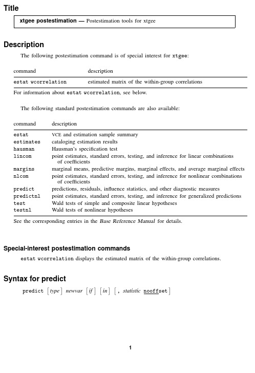
Titlextgee postestimation —Postestimation tools for xtgeeDescriptionThe following postestimation command is of special interest for xtgee :commanddescriptionestat wcorrelationestimated matrix of the within-group correlationsFor information about estat wcorrelation ,see below.The following standard postestimation commands are also available:command descriptionestatVCE and estimation sample summaryestimates cataloging estimation results hausman Hausman’s speciﬁcation testlincom point estimates,standard errors,testing,and inference for linear combinations of coefﬁcientsmargins marginal means,predictive margins,marginal effects,and average marginal effects nlcom point estimates,standard errors,testing,and inference for nonlinear combinations of coefﬁcientspredict predictions,residuals,inﬂuence statistics,and other diagnostic measurespredictnl point estimates,standard errors,testing,and inference for generalized predictions test Wald tests of simple and composite linear hypotheses testnlWald tests of nonlinear hypothesesSee the corresponding entries in the Base Reference Manual for details.Special-interest postestimation commandsestat wcorrelation displays the estimated matrix of the within-group correlations.Syntax for predictpredicttypenewvarifin,statistic nooffset12xtgee postestimation—Postestimation tools for xtgeestatistic descriptionMainmu predicted value of depvar;considers the offset()or exposure();the default rate predicted value of depvarpr(n)probability Pr(y j=n)for family(poisson)link(log)pr(a,b)probability Pr(a≤y j≤b)for family(poisson)link(log)xb linear predictionstdp standard error of the linear predictionscoreﬁrst derivative of the log likelihood with respect to x jβThese statistics are available both in and out of sample;type predict...if e(sample)...if wanted only for the estimation sample.MenuStatistics>Postestimation>Predictions,residuals,etc.Options for predict££Main mu,the default,and rate calculate the predicted value of depvar.mu takes into account the offset() or exposure()together with the denominator if the family is binomial;rate ignores those adjustments.mu and rate are equivalent if you did not specify offset()or exposure()when youﬁt the xtgee model and you did not specify family(binomial#)or family(binomial varname),meaning the binomial family and a denominator not equal to one.Thus mu and rate are the same for family(gaussian)link(identity).mu and rate are not equivalent for family(binomial pop)link(logit).Then mu would predict the number of positive outcomes and rate would predict the probability of a positive outcome.mu and rate are not equivalent for family(poisson)link(log)exposure(time).Then mu would predict the number of events given exposure time and rate would calculate the incidence rate—the number of events given an exposure time of1.pr(n)calculates the probability Pr(y j=n)for family(poisson)link(log),where n is a nonnegative integer that may be speciﬁed as a number or a variable.pr(a,b)calculates the probability Pr(a≤y j≤b)for family(poisson)link(log),where a andb are nonnegative integers that may be speciﬁed as numbers or variables;b missing(b≥.)means+∞;pr(20,.)calculates Pr(y j≥20);pr(20,b)calculates Pr(y j≥20)in observations for which b≥.and calculatesPr(20≤y j≤b)elsewhere.pr(.,b)produces a syntax error.A missing value in an observation of the variable a causes a missing value in that observation for pr(a,b).xb calculates the linear prediction.stdp calculates the standard error of the linear prediction.xtgee postestimation —Postestimation tools for xtgee 3score calculates the equation-level score,u j =∂ln L j (x j β)/∂(x j β).nooffset is relevant only if you speciﬁed offset(varname ),exposure(varname ),fam-ily(binomial #),or family(binomial varname )when you ﬁt the model.It modiﬁes the calculations made by predict so that they ignore the offset or exposure variable and the binomial denominator.Thus predict ...,mu nooffset produces the same results as predict ...,rate .Syntax for estat wcorrelationestat wcorrelation,compact format(%fmt )MenuStatistics>Postestimation>Reports and statisticsOptions for estat wcorrelationcompact speciﬁes that only the parameters (alpha)of the estimated matrix of within-group correlations be displayed rather than the entire matrix.format(%fmt )overrides the display format;see [D ]format .RemarksExample 1xtgee can estimate rich correlation structures.In example 2of [XT ]xtgee ,we ﬁt the model.use /data/r11/nlswork2(National Longitudinal Survey.Young Women 14-26years of age in 1968).xtgee ln_w grade age c.age#c.age (output omitted )After estimation,estat wcorrelation reports the working correlation matrix R :.estat wcorrelationEstimated within-idcode correlation matrix R:c1c2c3c4c5c6r11r2.48513561r3.4851356.48513561r4.4851356.4851356.48513561r5.4851356.4851356.4851356.48513561r6.4851356.4851356.4851356.4851356.48513561r7.4851356.4851356.4851356.4851356.4851356.4851356r8.4851356.4851356.4851356.4851356.4851356.4851356r9.4851356.4851356.4851356.4851356.4851356.4851356c7c8c9r71r8.48513561r9.4851356.485135614xtgee postestimation—Postestimation tools for xtgeeThe equal-correlation model corresponds to an exchangeable correlation structure,meaning that the correlation of observations within person is a constant.The working correlation estimated by xtgee is0.4851.(xtreg,re,by comparison,reports0.5140.)We constrained the model to have this simple correlation structure.What if we relaxed the constraint?To go to the other extreme, let’s place no constraints on the matrix(other than its being symmetric).We do this by specifying correlation(unstructured),although we can abbreviate the option..xtgee ln_w grade age c.age#c.age,corr(unstr)nologGEE population-averaged model Number of obs=16085Group and time vars:idcode year Number of groups=3913Link:identity Obs per group:min=1Family:Gaussian avg= 4.1Correlation:unstructured max=9Wald chi2(3)=2405.20 Scale parameter:.1418513Prob>chi2=0.0000ln_wage Coef.Std.Err.z P>|z|[95%Conf.Interval]grade.0720684.00215133.500.000.0678525.0762843age.1008095.008147112.370.000.0848416.1167775c.age#c.age-.0015104.0001617-9.340.000-.0018272-.0011936_cons-.8645484.1009488-8.560.000-1.062404-.6666923.estat wcorrelationEstimated within-idcode correlation matrix R:c1c2c3c4c5c6r11r2.43548381r3.4280248.55973291r4.3772342.5012129.54751131r5.4031433.5301403.502668.62162271r6.3663686.4519138.4783186.5685009.73060051r7.2819915.3605743.3918118.4012104.4642561.50219r8.3162028.3445668.4285424.4389241.4696792.5222537r9.2148737.3078491.3337292.3584013.4865802.4613128c7c8c9r71r8.64756541r9.5791417.73865951This correlation matrix looks different from the previously constrained one and shows,in particular, that the serial correlation of the residuals diminishes as the lag increases,although residuals separated by small lags are more correlated than,say,AR(1)would imply.Example2In example1of[XT]xtprobit,we showed a random-effects model of unionization using the union data described in[XT]xt.We performed the estimation using xtprobit but said that we could have used xtgee as well.Here weﬁt a population-averaged(equal correlation)model for comparison:xtgee postestimation—Postestimation tools for xtgee5 .use /data/r11/union(NLS Women14-24in1968).xtgee union age grade i.not_smsa south##c.year,family(binomial)link(probit)Iteration1:tolerance=.12544249Iteration2:tolerance=.0034686Iteration3:tolerance=.00017448Iteration4:tolerance=8.382e-06Iteration5:tolerance=3.997e-07GEE population-averaged model Number of obs=26200Group variable:idcode Number of groups=4434Link:probit Obs per group:min=1Family:binomial avg= 5.9Correlation:exchangeable max=12Wald chi2(6)=242.57 Scale parameter:1Prob>chi2=0.0000 union Coef.Std.Err.z P>|z|[95%Conf.Interval]age.0089699.0053208 1.690.092-.0014586.0193985grade.0333174.0062352 5.340.000.0210966.04553821.not_smsa-.0715717.027543-2.600.009-.1255551-.01758841.south-1.017368.207931-4.890.000-1.424905-.6098308year-.0062708.0055314-1.130.257-.0171122.0045706 south#c.year1.0086294.00258 3.340.001.0035727.013686_cons-.8670997.294771-2.940.003-1.44484-.2893592Let’s look at the correlation structure and then relax it:.estat wcorrelation,format(%8.4f)Estimated within-idcode correlation matrix R:c1c2c3c4c5c6c7 r1 1.0000r20.4615 1.0000r30.46150.4615 1.0000r40.46150.46150.4615 1.0000r50.46150.46150.46150.4615 1.0000r60.46150.46150.46150.46150.4615 1.0000r70.46150.46150.46150.46150.46150.4615 1.0000r80.46150.46150.46150.46150.46150.46150.4615r90.46150.46150.46150.46150.46150.46150.4615r100.46150.46150.46150.46150.46150.46150.4615r110.46150.46150.46150.46150.46150.46150.4615r120.46150.46150.46150.46150.46150.46150.4615c8c9c10c11c12r8 1.0000r90.4615 1.0000r100.46150.4615 1.0000r110.46150.46150.4615 1.0000r120.46150.46150.46150.4615 1.0000We estimate theﬁxed correlation between observations within person to be0.4615.We have many data(an average of5.9observations on4,434women),so estimating the full correlation matrix is feasible.Let’s do that and then examine the results:6xtgee postestimation—Postestimation tools for xtgee.xtgee union age grade i.not_smsa south##c.year,family(binomial)link(probit)>corr(unstr)nologGEE population-averaged model Number of obs=26200Group and time vars:idcode year Number of groups=4434Link:probit Obs per group:min=1Family:binomial avg= 5.9Correlation:unstructured max=12Wald chi2(6)=198.45 Scale parameter:1Prob>chi2=0.0000union Coef.Std.Err.z P>|z|[95%Conf.Interval]age.0096612.0053366 1.810.070-.0007984.0201208grade.0352762.0065621 5.380.000.0224148.04813771.not_smsa-.093073.0291971-3.190.001-.1502983-.03584781.south-1.028526.278802-3.690.000-1.574968-.4820839year-.0088187.005719-1.540.123-.0200278.0023904 south#c.year1.0089824.00348652.580.010.002149.0158158_cons-.7306192.316757-2.310.021-1.351451-.109787.estat wcorrelation,format(%8.4f)Estimated within-idcode correlation matrix R:c1c2c3c4c5c6c7 r1 1.0000r20.6667 1.0000r30.61510.6523 1.0000r40.52680.57170.6101 1.0000r50.33090.36690.40050.4783 1.0000r60.30000.37060.42370.45620.6426 1.0000r70.29950.35680.38510.42790.49310.6384 1.0000r80.27590.30210.32250.37510.46820.55970.7009r90.29890.29810.30210.38060.46050.50680.6090r100.22850.25970.27480.36370.39810.49090.5889r110.23250.22890.26960.32460.35510.44260.5103r120.23590.23510.25440.31340.34740.38220.4788c8c9c10c11c12r8 1.0000r90.6714 1.0000r100.59730.6325 1.0000r110.56250.57560.5738 1.0000r120.49990.54120.53290.6428 1.0000As before,weﬁnd that the correlation of residuals decreases as the lag increases,but more slowly than an AR(1)process.Example3In this example,we examine injury incidents among20airlines in each of4years.The data are ﬁctional,and,as a matter of fact,are really from a random-effects model.xtgee postestimation—Postestimation tools for xtgee7.use /data/r11/airacc.generate lnpm=ln(pmiles).xtgee i_cnt inprog,family(poisson)eform offset(lnpm)nologGEE population-averaged model Number of obs=80Group variable:airline Number of groups=20Link:log Obs per group:min=4Family:Poisson avg= 4.0Correlation:exchangeable max=4Wald chi2(1)= 5.27 Scale parameter:1Prob>chi2=0.0217 i_cnt IRR Std.Err.z P>|z|[95%Conf.Interval]inprog.9059936.0389528-2.300.022.8327758.9856487lnpm(offset).estat wcorrelationEstimated within-airline correlation matrix R:c1c2c3c4r11r2.46064061r3.4606406.46064061r4.4606406.4606406.46064061Now there are not really enough data here to reliably estimate the correlation without any constraints of structure,but here is what happens if we try:.xtgee i_cnt inprog,family(poisson)eform offset(lnpm)corr(unstr)nologGEE population-averaged model Number of obs=80Group and time vars:airline time Number of groups=20Link:log Obs per group:min=4Family:Poisson avg= 4.0Correlation:unstructured max=4Wald chi2(1)=0.36 Scale parameter:1Prob>chi2=0.5496 i_cnt IRR Std.Err.z P>|z|[95%Conf.Interval]inprog.9791082.0345486-0.600.550.9136826 1.049219lnpm(offset).estat wcorrelationEstimated within-airline correlation matrix R:c1c2c3c4r11r2.57002981r3.716356.41921261r4.2383264.3839863.35212871There is no sensible pattern to the correlations.We created this dataset from a random-effects Poisson model.We reran our data-creation program and this time had it create400airlines rather than20,still with4years of data each.Here are the equal-correlation model and estimated correlation structure8xtgee postestimation—Postestimation tools for xtgee.use /data/r11/airacc2,clear.xtgee i_cnt inprog,family(poisson)eform offset(lnpm)nologGEE population-averaged model Number of obs=1600Group variable:airline Number of groups=400Link:log Obs per group:min=4Family:Poisson avg= 4.0Correlation:exchangeable max=4Wald chi2(1)=111.80 Scale parameter:1Prob>chi2=0.0000 i_cnt IRR Std.Err.z P>|z|[95%Conf.Interval]inprog.8915304.0096807-10.570.000.8727571.9107076lnpm(offset).estat wcorrelationEstimated within-airline correlation matrix R:c1c2c3c4r11r2.52917071r3.5291707.52917071r4.5291707.5291707.52917071The following estimation results assume unstructured correlation:.xtgee i_cnt inprog,family(poisson)corr(unstr)eform offset(lnpm)nologGEE population-averaged model Number of obs=1600Group and time vars:airline time Number of groups=400Link:log Obs per group:min=4Family:Poisson avg= 4.0Correlation:unstructured max=4Wald chi2(1)=113.43 Scale parameter:1Prob>chi2=0.0000 i_cnt IRR Std.Err.z P>|z|[95%Conf.Interval]inprog.8914155.0096208-10.650.000.8727572.9104728lnpm(offset).estat wcorrelationEstimated within-airline correlation matrix R:c1c2c3c4r11r2.47331891r3.5240576.57488681r4.5139748.5048895.58407071The equal-correlation model estimated aﬁxed correlation of0.5292,and above we have correlations ranging between0.4733and0.5841with little pattern in their structure.xtgee postestimation—Postestimation tools for xtgee9Methods and formulasAll postestimation commands listed above are implemented as ado-ﬁles.Also see[XT]xtgee—Fit population-averaged panel-data models by using GEE[U]20Estimation and postestimation commands。

AUTODYN基础教程三

ANSYS AUTODYN 基础教程三
2013-8-9
3-1
添加标题基础培训三
• 1、欧拉求解器
• 2、起爆设置 • 3、流固耦合
2013-8-9
3-2
添加标题 AUTODYN 求解器类型
Lagrange
SPH
Euler
Shell
ALE
Beam
2013-8-9
3-3
添加标题欧拉求解器
• 网格固定在空间，材料通过单元流动； • 通常用于液体、气体和大变形物体。 • 带强度的多物质欧拉求解器(Eler Parts
Compute Motion of Interaction Nodes and Polygons
3-13
2013-8-9
添加标题多物质欧拉求解器填充材料 (2D)
• 物理空间填充：
• • • • • • •
抛物线填充：通过系数ABC定义抛物线；选择里面还是外面；选择材料；填充密度；填充内能；填充速度。
3-14
2013-8-9
添加标题多物质欧拉求解器填充材料 (2D)
有效路径
高能炸药
高能炸药
惰性材料
初始点
2013-8-9
初始点
无效路径
4-38
添加标题起爆设置
起爆时间
直接路径影响的范围
起爆点 B 没有正确计算
A
初始起爆点 #1 #2 #3
影响的范围区域 I 区域 II 区域 III
I
B
II
C
#2
#3
惰性材料
III
D
2013-8-9
#1
4-39
添加标题起爆设置

有关工作的英语励志句子

【导语】开始努⼒吧！在这个过程中你必须放弃很多东西，但你要明⽩它们都不是你最终想要的，你要相信在你成功以后，总有⼀天它们会再回来，⽽且⽐现在更美好！欢迎阅读©⽆忧考⽹为⼤家精⼼整理的“有关⼯作的英语励志句⼦”！更多相关讯息请关注©⽆忧考⽹！【篇⼀】有关⼯作的英语励志句⼦ 1、在以后的学习中，刻苦学习，拼搏进取。

In the later study, study hard, enterprising. 2、⼈的价值蕴藏在⼈的才能之中。

The value of a man is in the person's ability. 3、环境永远不会⼗全⼗美，消极的⼈受环境控制，积极的⼈却控制环境。

The environment will never be perfect, negative people affected by environmental control, positive people control environment. 4、就算前⾯有⼤风⼤浪，我们也要咬紧⽛关，⼤步向前，因为我们拥有青春。

Even if in front of the wind waves, we also want to bite the bullet, big step forward, because we have the youth. 5、⼈⼀定要受过伤才会沉默专注，⽆论是⼼灵或**上的创伤，对成长都有益处。

People must focus on injury will only silence, whether spiritual or physical trauma, are helpful to growth. 6、⽣命对某些⼈来说是美丽的，这些⼈的⼀⽣都为某个奋⽃。

Life for some people is beautiful, the person's life is a struggle. 7、⾃⼰去做吧。

MINITAB用的英语翻译

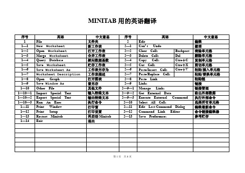
中文意思统计合适截取基本统计描述单样本（检验）相关（分析）协方差（分析）正态性试验回归分析回归分析逐步回归分析最小子集回归分析拟合线图残差图二元后勤回归顺序后勤回归名义后勤回归方差分析单变量方差分析单变量（非堆叠）双变量（方差分析）均值分析平衡数据方差分析遮盖分析
质量工具运行图泊拉图因果图能力分析能力六包量具运行图量具线性和偏倚研究重复性和再现性分析
共8页
MINITAB 用的英语翻译
序号 5—7 5—7—1 5—7—2 5—7—3 5—7—4 5—7—5 5—7—6 5—7—7 5—7—8 5—7—9 5—7—10 5—7—11 5—8 5—8—1 5—8—2 5—8—3 5—8—4 5—8—5 英语 DOE Greate Factoral Design Analyze Factoral Design Factoral Plots Greate RS Design Analyze RS Design RS Plots RS—Response Surface Greate Mixture Design Analyze Mixture Design Modify Design Display Design Analyze Custom Design Reliability/ Survival Distribution ID Plot Overview Plot Probability Plot Hazard Plot Survival Plot 中文意思实验设计生成因子设计分析因子设计因子图生成 RS 设计分析 RS 设计 RS 图响应表面生成混合设计分析混合设计混合图显示设计分析常规设计可靠性/继续生存性分布 ID 图概要图概率图危险图继续生存性图序号 5—9 5—9—1 5—9—2 5—9—3 5—8—4 5—9—5 5—9—6 5—10 5—10—1 5—10—2 5—10—3 5—10—4 5—10—5 5—10—6 5—10—7 5—10—8 5—10—9 5—10—10 5—10—11 5—10—12 5—10—13 英语 Multivariate Principal Components Factor Analysis Discriminant Analysis Cluster Observations Cluster Variables Cluster K—Means Time Series Time Series Plot Trend Analysis Decomposition Moving Average Single Exp Smoothing Double Exp Smoothing Winters Method Differences Lag Autocorrelation Partial Autocorrelation Cross Correlation ARIMA 中文意思多变量分析首要成分（分析）因子分析判别分析聚类观测聚类变量聚类 K—分组（分析）时间序列时间序列图趋势分析分解移动平均单指数平滑法双指数平滑法 Winters 方法差异滞后自相关局部自相关交叉相关 ARIMA 模型

时域计反射原理及应用

ZS L R L R
ES
C
G
C
G
ZL
Figure 2. The classical model for a transmission line.
The velocity at which the voltage travels down the line can be defined in terms of β: ω Unit Length per Second Where νρ = — β The velocity of propagation approaches the speed of light, νc, for transmission lines with air dielectric. For the general case, where er is the dielectric constant: νc νρ = —— √ er
2
and the nature (resistive, inductive, or capacitive) of each discontinuity along the line. TDR also demonstrates whether losses in a transmission system are series losses or shunt losses. All of this information is immediately available from the oscilloscope’s display. TDR also gives more meaningful information concerning the broadband response of a transmission system than any other measuring technique. Since the basic principles of time domain reflectometry are easily grasped, even those with limited experience in high-frequency measurements can quickly master this technique. This application note attempts a concise presentation of the fundamentals of TDR and then relates these fundamentals to the parameters that can be measured in actual test situations. Before discussing these principles further we will briefly review transmission line theory.

预测准确率

Example of MAPE calculation 平均绝对误差百分比计算
SKU A SKU B
Forecast 预测
75
Actual 实际
25
Error 误差
50
Error(%) 误差（%）
200%
Accuracy(%) 准确（%）
0%
0 50 50 100% 0%
SKU X 25 75 50 67% 33%
47%
46%
Root Mean Squared Error=
34
38
RMSE as % of Actuals =
61%
55%
Why MAPE ?为什么用平均绝对 Nhomakorabea差百分比？
MPE 平均误差百分比 •Very unstable 非常不稳定 •Will be skewed by small values 会被少数数值影响准确度 •In the Example ,SKU A drives most of the Error 在例子中，SKU A 占大多数的误差。 RMSE均方根误差 •Rigorous Error measure严格误差测量 •Not as easy as MAPE 不如平均绝对误差百分比那么容器 MAPE is simple and elegant while robust as a computational measure ! 平均绝对误差百分比是简单和优雅而强大的计算方法！
Long-term Forecast 长期预测
Market or economy-oriented市场或经济导向 Useful for 有用于 •Capacity Planning容量规划 •Setting Strategic initiatives 设置策略倡议 More flexibility to change and err更灵活地改变和犯错 Accuracy at an aggregate or macro level is more important 在聚合和宏的水平上精度更重要。 So mix matters less in Long-term forecasting ！所以在长期预测中，混合的问题更少。

Carrier HAP Transfer Function Methodology (TFM) 说明

Transfer Function Methodology (TFM)The Transfer Function Methodology (TFM) is a dynamic means of accountingfor heat transfer. Although there are other methods of accounting for heattransfer, Carrier’s HAP program utilizes TFM in its calculations because itextends the analysis to account for specific system behavior to control the airtemperature in the thermostat zones.This article will review the calculation methodology of TFM to assist ininterpreting the results of the HAP program. However, this article will notdiscuss the actual equations and formulas used. Such specific informationcan be found in the ASHRAE Fundamentals Handbook and in the HAP HelpSystem, Chapter 27: Load Calculations. See Figure 1.HAP e-Help has noticed that users of HAP have encountered two issues thatare preventing efficient use of the program. These issues are:• Consideration of load estimating as a steady-state, instantaneousoccurrence rather than a dynamic process•Expectation of results based on previous experience with other loadestimating programs that do not utilize TFM, especially those usingsimplifications to allow manual load calculations TFM is a derivative of the Heat Balance Method. Calculation shortcuts and assumptions are used to reduce the volume and detail of required input, and to speed up calculations. (See Section 27.2 in the HAP Online Help System.) Reduced input and faster calculations make this method more efficient. For example, the coefficients in Transfer Function equations are derived directly from a Heat Balance analysis. The Heat Balance equations are used once to derive Transfer Function coefficients, and the coefficients are used repeatedly to quickly calculateloads. (TFM does not use U-values for walls and roofs.)Conduction, convection, and radiation are the main drivers ofheat transfer to or from the air in the room. The resultingroom air temperature is calculated. The loads reported inHAP indicate how much cooling or heating is needed tomaintain the room temperature within the throttling range.What is described below may be a new way of consideringthe effects of heat gain and cooling load compared toprevious hand calculation methods adopted in the HVACengineering community. The methods used by HAP align withASHRAE calculation methodology.Figure 1 - HAP Online Help Figure 2 - Wall Heat Gain ExampleTransfer Function Methodology (TFM)The dynamics of heat gain over time are best described graphically. Because an east-facing wall (See Figure 2) is used in the example, the sol-air temperature curve shows the effects of large morning heat gains due to solar radiation and smaller afternoon heat gains due to reduced sunshine but warmer outdoor air temperatures. The heat gain curve reveals the transient heat transfer processes involved. While the sol-air temperatures peak at 8 a.m., the interior wall heat gains for this medium-weight wall do not peak until 2 p.m. This reveals the time it takes for heat to be conducted through this specific type of wall construction.Radiation heat gains from sources such as solar, lights and even people take time to become a load. The radiant heat must first heat up the building and contents and then be conducted and released over time to the room air by convection processes. This causes a delay between the time a heat gain occurs and the time its full effects as a cooling load appear.Figure 3 shows the load and heat gainsfor lights turned on for six hours. Note thatthe loads are smaller than the heat gainswhile the lights are on. This is because alarge portion of the heat gain is thermalradiation.Also note that cooling loads continue afterlights are turned off and the heat gainscease. Again, this is due to the radiantheat and the heat storage effects. Whenthe lights are turned off, some radiatedheat from the previous six hours is stillstored in the room mass and continues tobe convected to room air over time.Figure 3 - Lighting Heat Gain ExampleTransfer Function Methodology (TFM)Figure 4 - Peak Load Time LagFigure 4 illustrates that the Transfer Function Method models the transient build-up and discharge of heat in a building. The convection process is governed by the temperaturedifference between the mass and the room air. Convectiondecreases as the room air temperature rises and increasesas the room air temperature decreases. Hand calculationmethods assume a constant room air temperature at allhours to simplify this complex process. However, controlsystems have a throttling range, varying the room airtemperature. Using night set up or not cooling duringunoccupied times may cause an increase in roomtemperature and a decrease in convection, effectivelystoring heat for release. Later, on system start up, theroom air temperature rapidly decreases and a connectiverush of heat can occur. This is sometimes referred to as apull down load. See Figure 5. The TFM can calculate the effect of the changing room air temperature on the cooling and heating requirements. This is done using the Space Air Transfer functions referred to as Heat Extraction. This can be thought of as a thermostat and pulldown adjustment.Figure 5 - Peak Loads: 24 Hours versus 16 hoursTransfer Function Methodology (TFM)The transfer function with heat extraction is implemented in three steps and two stages in HAP.Stage OneStep One: The conduction equations are used to analyze the heat flow through walls and roofs.Step Two: The room transfer functions are used to analyze the radiative, convective and heat storage processes of all components. Convective components are instantaneous and radiative components are stored and released over time.Stage TwoStep Three: The space air temperature transfer functions (heat extraction equations) are used to analyze the effects of the changing room air temperature on convective heat flow from mass to room air that includes the behavior of the room thermostat.In the Stage One, Steps One and Two are completed assuming a constant room air temperature 24 hours. The components, control zones, and the system are sized. These components comprise the Zone and Space Loads reported in HAP. See Figures 7, 8, 9, and 10.In the Stage Two, Step three calculations are done. The system is simulated using the sizing from the first stage to correct the loads to what is needed to try to maintain set point. This is the “Zone Conditioning” reported in HAP (See Figures 7, 9, and 10.To illustrate the results of this procedure, Figure 6shows load, heat extraction, and room temperatureprofiles for a scenario in which HVAC equipmentoperates for the period 8 a.m. to 10 p.m., and is offfor the remaining hours of the day. Figure 6 showsthe cooling load profile calculated using the roomtemperature profile shows that during the 8 a.m. to10 p.m. operating period; the equipment maintainsthe zone within the thermostat throttling range of 72°F to 76°Figure 6 - Load, Heat Extraction, and Room Temperature Profiles period begins at 8 a.m., this accumulated heat isremoved in addition to the hourly cooling loads. Thisresults in a pulldown component of the load.Transfer Function Methodology (TFM)The HAP report “Air System Design Load Summary” (Figure 7) shows the results of the two stages of the calculation procedure. The Total Zones Loads are the results of Stage One. The “Zone Conditioning” and “Total Conditioning" results are from the Stage Two calculation.Figure 7 - Air System Design Load SummaryPage 6 of 9Transfer Function Methodology (TFM)The Zone DesignLoad Summaryand Space DesignLoad Summaryreports (Figure 8)show the detail ofthe Stage Oneresults.Figure 8 - Space Design Load Summary and Zone Design Load Summary ReportsTransfer Function Methodology (TFM)The Hourly Zone Loads report (Figure 9) shows the hourly results of the Stage One and Stage Two calculations as well as the varying hourly zone air temperature achieved.Figure 9 - Hourly Zone Load ReportTransfer Function Methodology (TFM)Graphing the column of numbers from the two stages can be done from the Hourly Zone Design Day Loads (see Figure 10). The magnitude of the pull down load can be seen at 6 am. The extra amount of “conditioning” represents the true demand for cooling needed for running 11 hours instead of 24 can easily be seen.Figure 10 - Hourly Design and Day LoadsTransfer Function Methodology (TFM)As a review, when performing calculations to determine required airflow rates, supply terminal characteristics, and coil capacities for HVAC systems, HAP uses the following general eight-step procedure:1. Compute sensible and latent loads for all zones served by the HVAC system.2. Sum zone loads to obtain sensible and latent loads for the HVAC system.3. Determine required zone airflow rates.4. Compute required sizes for terminal reheat coils as necessary.5. Determine required system airflow rates. This includes sizing all fans and outdoor ventilation airflow rates.6. Simulate HVAC system operation. Based on the required airflow rates determined in Steps 3 through 5. Operation ofthe HVAC system is mathematically simulated to produce profiles of loads on central cooling and heating coils.7. Identify peak coil loads. Cooling and heating coil load profiles from Step 6 are inspected to identify maximum loads.8. Report results.The results of these calculations can yield important benefits such as the ability to analyze the realistic transient heat transfer that occurs in all buildings. Loads can also be accurately computed for any heat gain sequence and wall or roof construction. Consequently, resulting loads are specific and customized for each application analyzed, accounting for local weather conditions, building construction and operating schedules. The value of these benefits is obvious for HVAC design work.Further articles in this series of HAP e-Help will build upon this discussion and explore how the HAP software can assist system design rather than just load calculation.。

Workbench AutoDYN系列教程3

拉格朗日 Parts
2015-3-10
填充的欧拉网格
多物质欧拉求解器
填充材料例子(3D)
• 使用Part Fill 填充复杂的形状：
拉格朗日 Parts
2015-3-10
填充的欧拉材料位置
欧拉求解器
欧拉边界条件
• 对于在边界条件上的欧拉单元，缺省的边界条件是刚性墙 (没有流动，速度 = 0.0)； • 空单元网格同样需要定义边界条件。
2015-3-10
起爆设置
起爆时间
间接的单点起爆
在阴影区域的爆炸时间精确计算
2015-3-10
起爆设置
起爆时间
间接的多点起爆
在阴影区域的爆炸时间计算
2015-3-10
起爆设置
• 起爆类型：2D和3D； • 起爆方式： • 2D：点、直线、圆环、手工设
置；
• 3D：点、平面、圆柱面、球面、手工设置。
2015-3-10
欧拉-拉格朗日耦合
• 欧拉施加压力给拉格朗日多边形； • 拉格朗日多边形给欧拉施加流动边界； • 使用精确的耦合算法(Euler 和 Euler-FCT)； • 不考虑摩擦； • 局部接触力通过接触段积分； • 部分覆盖单元被合并-“混合”。
欧拉-拉格朗日耦合
Pre and Post Processing Carry out Edits Compute Time Step
Calculate Interaction of Lagrangian Parts
Process Euler Parts
Compute Motion of Interaction Nodes and Polygons
2015-3-10
多物质欧拉求解器

网络计划技术虚箭线

• （1）A完成后c开始，A、B完成后D开始
A
B C D
（2）C随A，G随B，A、B完成后D开始
A
C
D
B
G
• (3) C随A、B; E随B、D
A B C
D
E
• (4) D随A、B、C, E随B、C
A B D E
C
• (5)有A、B两项工作，按三个施工段进行流水施工
A1 A2 A3
B1
B2
1
2 5
3
4
• 6.虚箭线的应用
⑤ A完成后进行C， A、B均完成后进行D。
⑥A、B均完成后进行D，
A、B、C均完成后进行E， D、E均完成后进行F。
具体如何画图虚箭线应用
⑤
1
A B
3
C D
5
2
4
6
⑥
1 2
A B C
4
D E F
3
5
6
7
做练习
（1）A完成后C开始，A、B完成后D开始（2）C随A，G随B，A、B完成后D开始 (3) C随A、B; E随B、D (4) D随A、B、C; E随B、C (5)有A、B两项工作，按三个施工段进行流水施工
C 1
5 4 6
G 7 F H 8
A
2
B
3
E D
练习1：已知各工序之间逻辑关系如下表，试绘双代号网络图。
工序紧前工作紧后工作 A B C D ABC E BC F C G DE H E I EF
练习2
工作名称 A B C D E F G H I
紧前工作
-
-
-
B
BC
C
AD

1、下载文档前请自行甄别文档内容的完整性，平台不提供额外的编辑、内容补充、找答案等附加服务。
2、"仅部分预览"的文档,不可在线预览部分如存在完整性等问题,可反馈申请退款(可完整预览的文档不适用该条件!)。
3、如文档侵犯您的权益，请联系客服反馈,我们会尽快为您处理(人工客服工作时间：9:00-18:30)。

TypeO.D(")I.D(")Length(m)linear(")Stroke(")Efficiency(%)
218.00DC182.8856.1256pump16.712100
218.00DC272.76134.30134pump26.712100
12.25HWDP62.7627.5829
I.D(")12.62DP
54.250.00

shoe(m)211.29Surface
53.6054.86

Vpm(ft/min)
100

114
DC1/OH6.71mSPM214Mud Weight8.84ppgDiameter(")
0.2364

DC1/CSG49.41mPump165316PV20Thickness(")
0.0788

DC2/OH0mPump26540YP9ROP(ft/hr)
15

DC2/CSG134.30mGPM50θ60058S.G.C(g/cc)
2.5

HWDP/OH0mFlowIn
714.291160θ30038

HWDP/CSG27.58m
2703.87770θ64

DP/OH0m
l/min80θ33

DP/CSG0m
90

100

4.40min

Last casing
bbls/stroke
Hole Diameter(")

BHALag timeSwab and SurgeCuttings CharacterPumps dataHOLE0.1310.131Pump Data

Basic data input area

Jet(/32")
Hole dataMud properties

M.D.(m)
TVD(m)