(完整word版)Maxwell与Simplorer联合仿真方法及注意问题
maxwell电机仿真实例

maxwell电机仿真实例Maxwell电机仿真是模拟电机运行情况的一种重要方法,通过仿真得到电机的性能参数,用于电机的设计优化以及电机控制系统的开发。
下面以一台交流电机为例,介绍Maxwell电机仿真实例。
一、仿真前的准备工作在进行仿真前,需要准备以下的工作:1.电机几何模型:需要准确建立电机的几何模型,包括电机的结构、尺寸和材质等。
2.电机的材料特性:需要准备电机的材料特性,比如磁导率、电导率等。
3.电机所需的控制模型:需要准备电机控制模型,包括电机的控制器、传感器、电源等。
4.仿真平台的选择:需要选择合适的仿真软件,Maxwell是一款专为电机设计和仿真而开发的软件,因此是一个很好的选择。
二、建立电机的几何模型电机的几何模型主要由电机的结构、尺寸和材质等组成。
在Maxwell中,可以通过几何建模工具对电机进行建模,建立好几何模型后,可以对电机的各个部分进行编辑和修改,满足不同的需求。
三、添加电机材料特性添加电机材料特性主要是设置电机的材料属性,比如磁导率、电导率等。
这些属性决定了电机在磁场中的反应和电磁参数。
在Maxwell 中,可以通过设置材料属性来实现。
四、设置仿真参数在进行仿真前,需要设置仿真的参数,比如电机的工作条件、电机的输入电流等。
在Maxwell中,可以根据需要设置仿真的参数,并可根据仿真结果进行优化。
五、仿真结果分析仿真分析实际上就是将仿真结果用图像或者图表的形式呈现出来,以便于对比和分析。
Maxwell电机仿真分析的结果包括:1.电机的电磁参数:包括电机的电感、电阻、电机的空载电流等。
2.电机的磁力:包括发生在电机各部分的磁力的大小和方向等。
3.电机的机械参数:包括电机的转速、效率、压力等。
通过仿真分析得到的结果,可以用于电机设计和仿真的优化,也可以用于控制系统的开发。
六、结论Maxwell电机仿真是电机设计和控制系统开发的一种重要方法,通过仿真可以得到电机的性能参数。
仿真前需要进行准备工作,包括建立电机的几何模型、添加电机材料特性、设置仿真参数等。
(完整)Maxwell仿真实例
MAXWELL 3D 12。
0BASIC EXERCISES1. 静电场问题实例:平板电容器电容计算仿真 (1)2. 恒定电场问题实例:导体中的电流仿真 (5)3. 恒定磁场问题实例:恒定磁场力矩计算 (10)4。
参数扫描问题实例:恒定磁场力矩计算 (15)5. 恒定磁场实例:三相变压器电感计算 (23)6. 永磁体磁化方向设置:局部坐标系的使用 (33)7. Master/Slave边界使用实例:直流无刷电机内磁场计算 (39)8. 涡流场分析实例 (46)9. 涡流场问题实例:磁偶极子天线的近区场计算 (54)10。
瞬态场实例:TEAM WORKSHOP PROBLEM 24 (59)1。
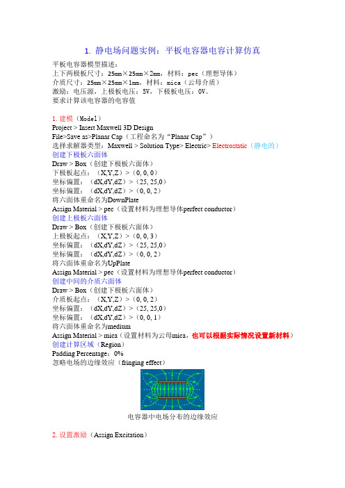
静电场问题实例:平板电容器电容计算仿真平板电容器模型描述:上下两极板尺寸:25mm×25mm×2mm,材料:pec(理想导体)介质尺寸:25mm×25mm×1mm,材料:mica(云母介质)激励:电压源,上极板电压:5V,下极板电压:0V.要求计算该电容器的电容值1.建模(Model)Project > Insert Maxwell 3D DesignFile〉Save as>Planar Cap(工程命名为“Planar Cap")选择求解器类型:Maxwell > Solution Type> Electric> Electrostatic 创建下极板六面体Draw 〉 Box(创建下极板六面体)下极板起点:(X,Y,Z)>(0, 0, 0)坐标偏置:(dX,dY,dZ)〉(25, 25,0)坐标偏置:(dX,dY,dZ)〉(0, 0, 2)将六面体重命名为DownPlateAssign Material > pec(设置材料为理想导体perfect conductor)创建上极板六面体Draw > Box(创建下极板六面体)上极板起点:(X,Y,Z)>(0, 0, 3)坐标偏置:(dX,dY,dZ)>(25, 25,0)坐标偏置:(dX,dY,dZ)>(0, 0, 2)将六面体重命名为UpPlateAssign Material > pec(设置材料为理想导体perfect conductor)创建中间的介质六面体Draw > Box(创建下极板六面体)介质板起点:(X,Y,Z)〉(0, 0, 2)坐标偏置:(dX,dY,dZ)>(25, 25,0)坐标偏置:(dX,dY,dZ)〉(0, 0, 1)将六面体重命名为mediumAssign Material 〉 mica(设置材料为云母mica,也可以根据实际情况设置新材料)创建计算区域(Region)Padding Percentage:0%忽略电场的边缘效应(fringing effect)电容器中电场分布的边缘效应2。
Maxwell仿真实例
1. 静电场问题实例:平板电容器电容计算仿真平板电容器模型描述:上下两极板尺寸:25mm×25mm×2mm,材料:pec(理想导体)介质尺寸:25mm×25mm×1mm,材料:mica(云母介质)激励:电压源,上极板电压:5V,下极板电压:0V。
要求计算该电容器的电容值1.建模(Model)Project > Insert Maxwell 3D DesignFile>Save as>Planar Cap(工程命名为“Planar Cap”)选择求解器类型:Maxwell > Solution Type> Electric> Electrostatic(静电的)创建下极板六面体Draw > Box(创建下极板六面体)下极板起点:(X,Y,Z)>(0, 0, 0)坐标偏置:(dX,dY,dZ)>(25, 25,0)坐标偏置:(dX,dY,dZ)>(0, 0, 2)将六面体重命名为DownPlateAssign Material > pec(设置材料为理想导体perfect conductor)创建上极板六面体Draw > Box(创建下极板六面体)上极板起点:(X,Y,Z)>(0, 0, 3)坐标偏置:(dX,dY,dZ)>(25, 25,0)坐标偏置:(dX,dY,dZ)>(0, 0, 2)将六面体重命名为UpPlateAssign Material > pec(设置材料为理想导体perfect conductor)创建中间的介质六面体Draw > Box(创建下极板六面体)介质板起点:(X,Y,Z)>(0, 0, 2)坐标偏置:(dX,dY,dZ)>(25, 25,0)坐标偏置:(dX,dY,dZ)>(0, 0, 1)将六面体重命名为mediumAssign Material > mica(设置材料为云母mica,也可以根据实际情况设置新材料)创建计算区域(Region)Padding Percentage:0%忽略电场的边缘效应(fringing effect)电容器中电场分布的边缘效应2.设置激励(Assign Excitation)选中上极板UpPlate,Maxwell 3D> Excitations > Assign(计划,分配)>Voltage > 5V选中下极板DownPlate,Maxwell 3D> Excitations > Assign >Voltage > 0V3.设置计算参数(Assign Executive Parameter)Maxwell 3D > Parameters > Assign > Matrix (矩阵)> Voltage1, Voltage2 4.设置自适应计算参数(Create Analysis Setup)Maxwell 3D > Analysis Setup > Add Solution Setup最大迭代次数:Maximum number of passes > 10误差要求:Percent Error > 1%每次迭代加密剖分单元比例:Refinement per Pass > 50%5. Check & Run6. 查看结果Maxwell 3D > Reselts > Solution data > Matrix电容值:31.543pF2. 恒定电场问题实例:导体中的电流仿真恒定电场:导体中,以恒定速度运动的电荷产生的电场称为恒定电场,或恒定电流场(DC conduction (传导)) 恒定电场的源:(1)Voltage Excitation ,导体不同面上的电压 (2)Current Excitations ,施加在导体表面的电流(3)Sink (汇),一种吸收电流的设置,确保每个导体流入的电流等于流出的电流。
Simplorer和Matsimulink联合仿真

Simplorer和Matsimulink联合仿真Matlab/simulink和Simplorer联合仿真Matlab/simulink和Simplorer联合仿真的意义在于:Simplorer 可以调用simulink中已经建好或者封装好的子模块进行联合仿真,利用现有的模型,为仿真提供便利。
Sim2Sim 指Ansoft/Simplorer与Matlab/Simulink 之间的联合仿真。
本人使用的分别是Simplorer 9.0和Matlab R2010a版本。
打开 SIMPLORER9.0 的安装路径,在 cpl 文件夹下的matlab 文件夹中可以看到Simplorer 9.0支持的联合仿真的Matlab 的版本,如下图所示:图1进入到与R2010a文件夹下,会看到3个文件,见图2。
其中AnsoftLinkDialog.m文件实现对另外两个文件的操作,而AnsoftSFunction 函数正是实现Simulink 与Simplorer 数据传输的桥梁。
图2在进行Sim2Sim 联合仿真之前,先要将图中三个文件所在的路径加载到Matlab的扫描路径中,见图3、4。
因为Matlab 在运行一个函数的时候,只会在自己的扫描路径内搜索,如果不在其扫描路径内,就找不到相应的函数,因此就不会执行,这一点Matlab的通性。
记住Ansoft 的软件不支持中文路径和中文文件名。
图3图4联合仿真过程如下:1.Simplorer中的操作(1)在Simplorer 9.0中建立工程,保存为connect_sim.amsp;(2)添加Simulink 连接部件,见图5,弹出图6示的窗口;图6(3)点击图 6中所示红色圈出的按钮,添加 Simulink 部件的变量,输入变量名为feedback ,默认值为0,选择to simulink 作为其输入变量;同理,添加simulink的输出变量PWM,界面如图7所示。
labview和simulink联合仿真方法(功能测试)
labview和simulink联合仿真⽅法(功能测试)由于Simulink模型在仿真过程中不能实时修改参数,导致在进⾏功能仿真时效率很低,⽽利⽤labview的SIT模块可以在仿真的过程中实时修改和查看参数,提⾼仿真效率。
⼀、利⽤labview SIT模块与Simulink联合仿真。
软件环境:labview2012、matlab r2011b操作步骤1. ⾸先安装matlab软件2. 先安装labview2012,然后安装SIT(Simulink interface toolkit)模块。
必须安装labview2012或之前的版本,因为之后的版本不再⽀持SIT。
1. 设置labview。
新建⼀个空⽩VI;打开⼯具/选项/VI服务器;选择TCP/IP,在机器访问列表中输⼊本机IP或者localhost,选择⼯具/SIT connection manager设置vi服务器端⼝:6011在current Model处选择要仿真的mdl模型;下⾯选择⼯程的路径;点击OK⽣成仿真程序。
1. 设置MATLAB打开MATLAB软件,输⼊edit matlabrc命令,将以下命令添加到⽂件末尾:addpath('D:\SimulationInterfaceToolkit');%添加SIT安装路径NISIT_AddPaths;NISITServer;%启动NIserver保存后重新打开MATLAB,命令窗⼝出现:SIT: Added paths for Simulation Interface Toolkit Version 2012Starting the SIT Server on port 6011SIT Server started表⽰已经与服务器连接。
1. 设置mdl模型打开要仿真的模型,选择Simulation/configuration parameters/code generation在system target file中选择nidll.tlc,使⽤NI规则⽣成代码。
maxwell和workbench的联合仿真

Coupling Maxwell Designs with ANSYS Thermal viaWorkbenchCoupling Maxwell2D/3D V15 with ANSYS R14 is supported via the Workbench schematic. Thermal feedback is supported for Maxwell magnetostatic, eddy current, and transient types. Users also need to setup the design and geometry appropriately. An appropriate design should be temperature-dependent, and have one or more solve setups that are enabled for thermal feedback.1. The easiest way to add a Maxwell 2D or 3D design to a Workbench schematic isto import a working design via Workbench File>Import. The imported design is placed in the Workbench schematic after it is successfully imported.2. Next, insert a Steady-State Thermal system and change its Analysis Type to 2D or 3D, (depending on the Maxwell design type) by right clicking on the Geometry cell and selecting Properties. It is important to change the Steady-State Thermal system's analysis type before setting up its geometry.3. To setup the Steady-State Thermal system's geometry, you must first export the Maxwell geometry using sat or step format as follows:a. Select the Modeler>Export menu item.b. Select the desired model geometry format (sat or step), and the save location in the dialog box and save the file for use by ANSYS Workbench.4. Import the file via the Geometry module of the Steady-State Thermal system.a. To access the Geometry module, double click on the Geometry cell in the Steady-State Thermal system to launch DesignModeler.b. Select File>Import External Geometry File and browse for the geometry file exported from Maxwell.c. After the geometry file is imported, right-click on the root folder of the modeler project tree and select Generate. (When the geometry file is of a Maxwell 2D RZ design, users can rotate the geometry in DesignModeler by creating a body operation.)5. Close DesignModeler and refresh the Model cell of the Steady-State Thermal system by right-clicking the Model cell and selecting Refresh.6. The geometry mode of the Steady-State Thermal system can be changed via the ANSYS Mechanical user interface.a. Launch Mechanical by double clicking the Setup cell of the Steady-State Thermal system.b. Select Geometry in the project tree and the Definition of Geometry will be shown in the Detail window.c. Select either Plane Stress or Axisymmetric as the value for the property 2D (or 3D) Behavior.7. To setup the coupling, drag the Solution cell of the Maxwell system and drop it on the Setup cell of the Steady-State Thermal system.8. Note that the Maxwell Solution cell is tagged with a “Lighting Bolt” symbol. Right-click on the Maxwell Solution cell and select Update. This will initiate a Maxwell simulation if it is not already solved. Once Maxwell's solution is available, the “Lighting Bolt” changes to a “Green Check”symbol.9. To “push” the coupling into Steady-State Thermal, right-click on the Steady-State Thermal Setup cell and select Refresh.10. After refresh is finished, you can launch ANSYS Mechanical by double-clicking the Setup cell to finish the coupling setup.11. In the ANSYS Mechanical application project tree, an Imported Load(Maxwell2DSolution), or (Maxwell3DSolution), item should already be inserted. Select the Imported Load folder to view its details. Because the inserted Maxwell2D (or 3D) system supports thermal feedback, the Details window shows information regarding how the temperature result should be exported, and what type of mesh mapping should be used.12. To finish the coupling setup, you must insert either an imported Heat Generation or an imported Heat Flux boundary condition. Heat Generation is usedwhen mapping loss from objects in Maxwell; and Heat Flux should be used to map the loss from the edges of objects in Maxwell. Users can insert multiple Heat Generation or Heat Flux loads via the Imported Load (Maxwell2DSolution), or Imported Load(Maxwell3DSolution) objects.13. To insert a Heat Generation, use Body select by clicking the icon in theMechanical Toolbar. Then click on the objects where the EM loss should be imported. After all the desired objects are selected, right-click on Imported Load (Maxwell2DSolution)> Insert > Heat Generation, or ImportedLoad(Maxwell3DSolution) > Insert > Heat Generation.A sub-item named Imported Heat Generation will appear in the project tree.14. Click on the Imported Heat Generation tree item to view its details.15. In the Transfer Definition section, users can setup the source Maxwell solution by pulling down the Ansoft Solution combo box and select one of the listed Maxwell solutions.16. Right-clicking on Imported Heat Generation > Import Load will import loss from the Ansoft Solution selected for this load. After import has completed, the Import Heat Generation item becomes a folder, and an entry called Imported Load Transfer Summary is listed. Select the Imported Load Transfer Summary entry and the scaling factors used to export the load from Maxwell will be displayed in the Comment window.17. Selecting Import Heat Generation should show an overlay-plot of the imported load. The loss mapping from Maxwell can be verified by comparing this overlay-plot with an Ohmic-Loss field overlay plot in Maxwell.18. Create a Convection boundary to complete the thermal setup. Use Edge select by clicking the icon at the Mechanical Toolbar and then Edit > Select All.With the edges selected, right-click on the Steady-State Thermal project tree item and insert a Convection. With the Convection item selected, change its Film Coefficient to 5 W/m2 via the Detail window. Right-click on the Solution tree item and select Solve. After the thermal solution is finished, users can insert a Temperature plot by right-clicking on Solution and selecting Insert > Thermal > Temperature. Right-click on the newly inserted Temperature item and select Evaluate All Results.19. To export the thermal result to Maxwell, right-click on the Imported Load (Maxwell2DSolution), or Imported Load(Maxwell3DSolution) and select Export Results.20. To fully utilize the automation capabilities provided in ANSYS Workbench, select Imported Load (Maxwell2DSolution), or Imported Load(Maxwell3DSolution); and in its Detail window, select Yes for Export after Solve. With this option selected, users can continue the iteration between Maxwell/Thermal simulations from the Workbench schematic.To “push” the exported thermal results back to Maxwell, right-click on Maxwell's Solution cell on the Workbench schematic and select Enable Update. Then, right-click again on Maxwell's Solution cell and select Update. This will trigger Maxwell to re-simulate its solution with thermal results.To continue the solve iterations, repeat the following steps as needed:a. Right-click on Thermal's Setup cell and select Refresh.b. Right-click on Thermal's Setup cell and select Update.c. Right-click on Maxwell's Solution cell and select Enable Update.d. Right-click on Maxwell's Solution cell and select Update.Coupling Maxwell Designs with ANSYS Structural viaWorkbenchStress feedback coupling between Maxwell2D/3D V15 and ANSYS Structural R14 is supported via the Workbench schematic. Stress feedback is supported for Maxwell magnetostatic, eddy current, and transient types. Users also need to setup the design and geometry appropriately. An appropriate design has one or more solve setups that are enabled for stress feedback. The process for stress feedback coupling between Maxwell and ANSYS Structural is similar to that described in “Coupling Maxwell Designs with ANSYS Thermal via Workbench”.1. The easiest way to add a Maxwell 2D or 3D design to a Workbench schematic isto import a working design via Workbench File>Import. The imported design is placed in the Workbench schematic after it is successfully imported.2. Next, insert a Static Structural system and change its Analysis Type to 2D or 3D, (depending on the Maxwell design type) by right clicking on the Geometry cell and selecting Properties. It is important to change the Steady-State Thermal system's analysis type before setting up its geometry.3. To setup the Static Structural system's geometry, you must first export the Maxwell geometry using sat or step format as follows:a. Select the Modeler>Export menu item.b. Select the desired model geometry format (sat or step), and the save location in the dialog box and save the file for use by ANSYS Workbench.4. Import the file via the Geometry module of the Static Structural system.a. To access the Geometry module, double click on the Geometry cell in the Static Structural system to launch DesignModeler.b. Select File>Import External Geometry File and browse for the geometry file exported from Maxwell.c. After the geometry file is imported, right-click on the root folder of the modeler project tree and select Generate. (When the geometry file is of a Maxwell 2D RZ design, users can rotate the geometry in DesignModeler by creating a body operation.)5. Close DesignModeler and refresh the Model cell of the Static Structuralsystem by right-clicking the Model cell and selecting Refresh.6. The geometry mode of the Static Structural system can be changed via the ANSYS Mechanical user interface.a. Launch Mechanical by double clicking the Setup cell of the Static Structural system.b. Select Geometry in the project tree and the Definition of Geometry will be shown in the Detail window.c. Select either Flexible or Rigid as the value for the property 2D (or 3D) Stiffness Behavior.7. To setup the coupling, drag the Solution cell of the Maxwell system and dropit on the Setup cell of the Static Structural system.8. Note that the Maxwell Solution cell is tagged with a “Lighting Bolt” symbol. Right-click on the Maxwell Solution cell and select Update. This will initiate a Maxwell simulation if it is not already solved. Once Maxwell's solution is available, the “Lighting Bolt” changes to a “Green Check”symbol.9. To “push” the coupling into Static Structural, right-click on the Static Structural Setup cell and select Refresh.10. After refresh is finished, you can launch ANSYS Mechanical by double-clicking the Setup cell to finish the coupling setup, which is similar to that describedin “Coupling Maxwell Designs with ANSYS Thermal via Workbench”.Coupling Maxwell with Both ANSYS Thermal and Structural via WorkbenchA Maxwell system can also be coupled with both thermal and stress systems via Workbench. The thermal system then serves as an “up-stream” system for the stress system. This means that the stress analysis takes both electromagnetic and thermal forces into consideration. In this scenario the user must select the same object(s) in the thermal and stress systems to apply the respective imported loads.To setup the coupling, drag the “Solution” cell of the Maxwell system and drop it at the “Setup” cell of a Thermal and Static Structural (Stress) system. The user also needs to couple the Thermal and Static Structural systems to capture the effect of thermal force.The coupling framework is built on top of the existing Thermal Feedback. The Stress system will have additional Export Definition and Mapping Settings like Thermal.Example 1: “One” iterationThe image below illustrates a coupling setup where both the Thermal and Stress system are ready to be Updated. The Maxwell adaptive solution has converged in 3 passes. The Maxwell system has both thermal and stress feedback enabled.1. Right click on the Solution cell of Stress (Static Structural) and select Update.a. The Setup of The rmal will be Updated with “em” loss from Maxwell.b. The Solution of Thermal will be Updated and temperature will be exported to Maxwell.c. The Setup of Stress will be Updated with thermal force from Thermal and force density from Maxwell.d. Displacement will be exported to Maxwell after Stress finishes simulation.2. Right click on the Solution cell of Maxwell and select Enable Update.3. Right click on the Solution cell of Maxwell and select Update.a. Maxwell re-simulates the 3rd pass with its mesh and thetemperature/displacement feedback.b. The profile will show information about the feedbackc. Both Revert to Initial Temperature and Revert to Zero Displacement menus are present in the analysis setup context menu.Example 2: Manual iterationThe image below illustrates the Workbench schematic after Example 1, where the 1st iteration has completed.1. Right click on the Solution cell of Stress and select Update.a. The Setup of Thermal will be Refreshed and Updated with “em” loss from Maxwell.b. The Solution of Thermal will be Updated and temperature will be exported to Maxwell.c. The Setup of Stress will be Refreshed and Updated with thermal force from Thermal and force density from Maxwell.d. Displacement will be exported to Maxwell after Stress finishes simulation.2. Right-click on the Solution cell of Maxwell and select Enable Update.3. Right-click on the Solution cell of Maxwell and select Update.a. Maxwell re-simulates the 3rd pass with its mesh and newtemperature/displacement feedback.b. The profile will show information about the feedback.Note that the delta temperature and displacement is being reported in the profile.Example 3: Revert Maxwell SolutionThe temperature and displacement in the Maxwell solution can be reverted separately.1. Users select Revert to Initial Temperature in Maxwell.A warning message displays notifying users about the invalidation of solution.2. Right-click on Maxwell analysis setup and select Analyze.Maxwell re-simulates the 3rd pass with its mesh and displacement that was previously exported from Mechanical, but without temperature.3. Users select Revert to Zero Displacement in Maxwell, followed by right-clicking on Maxwell analysis setup and selecting Analyze.Maxwell re-simulates the 3rd pass with its mesh without either temperature nor displacement.Example 4: Only Stress FeedbackThe coupling setup is the same as in Example 1, with either one of the following differences:•The Maxwell system is not enabled for thermal feedback (via SetObjectDisplacement). Note that since Maxwell is not enabled to support feedback, the “Export Result” proper ties should be available in the thermal system.•The Maxwell system is enabled for thermal feedback, but users choose not to “Export Result’ in the thermal system. This is to disable the automatic “Export Results”.1. Right click on the Solution cell of Stress and select Update.a. The Setup of Thermal will be Updated with “em” loss from Maxwell.b. The Solution of Thermal will be Updated.c. The Setup of Stress will be Updated with thermal force from Thermal and force density from Maxwell.d. Displacement will be exported to Maxwell after Stress finishes simulation.2. Right-click on the Solution cell of Maxwell and select Enable Update.3. Right-click on the Solution cell of Maxwell and select Update.a. Maxwell re-simulates the 3rd pass with its mesh and the displacement feedback.b. The profile shows information about the feedback and Revert to Zero Displacement will be available in the solve setup context menu.。
联合仿真常见错误

联合仿真常见错误在建立adams与matlab的连接时,要导出adams模型,点击controls/plant export命令,创建输入输出变量,并生成三个文件,为aa.m aa.cmd和aa.adm文件。
(.m文件保存输入输出信息,.cmd 文件为命令文件,.adm为数据文件)其中aa为file prefix框中的内容,即导出模型的文件名。
在matlab下输入adams_sys,创建系统控制模型。
联合仿真常见错误归纳1、将…\MSC.ADAMS\2005\Win32\文件夹中的adams_plant.dll文件和…\MSC.ADAMS\2005\Controls->Win32\下的plant.lib文件也Copy到 matlab的工作目录下。
2、前一次的仿真出错,虽然修改了matlab模块,但matlab工作空间内的信息没有修改。
解决办法是在matlab命令行中键入:clear all回车XXX.m回车adams_sys回车从而,重新打开模块。
3、还有检查一下adams界面中,建立控制模块的 control plant的adams host 是否为本机名。
4、检查m文件中路径“\”与“/”的错误,这是系统自动生成文件时的bug,只有手动修改。
5、如果有上网的客户端认证软件建议在仿真之前把它关掉,因为经常出现ADAMS的server不能开启的情况,关掉认证软件后,就能执行了。
一般一些校园网上网时比较容易用这些客户端认证软件,比如华为的。
6、把ADAMS的工作路径直接设置到MATLAB的work文件夹中,避免路径出错7、修改.m文件中的flag==08、有时由于参数不正确等原因,仿真会失败,比如提示如下错误:Error reported by S-function 'adams_plant' in'GCdd/adams_sub/ADAMS Plant/S-Function': ADAMS output uation failure at time 0.695000。
matlab(simulink)+simplorer+maxwell 电机联合仿真 svpwm EMIl滤波器 差共模信号分离

பைடு நூலகம்
EMI Filter
Electrical equipments are widely used in our daily life. They bring great convenience to our life and also make our electromagnetic environment more and more complex. EMI filter is a method to solve the problem of electromagnetic compatibility(电磁兼容). In this project, my work is to find a circuit to separate common mode signal and differential mode signal(共差模信号).
Simulation
Simulation stop time at 100ms (5 periods), the minimum step 10us. The computer runs for about 240 hours to complete it. Results as follows:
Main Idea
Operating Frequency: 150kHz – 30MHz
High-pass filter(高通滤波器) (to filter signals below 150kHz)
High-frequency transformer(高频变压器) (separate common mode signal and differential mode signal)
- 1、下载文档前请自行甄别文档内容的完整性,平台不提供额外的编辑、内容补充、找答案等附加服务。
- 2、"仅部分预览"的文档,不可在线预览部分如存在完整性等问题,可反馈申请退款(可完整预览的文档不适用该条件!)。
- 3、如文档侵犯您的权益,请联系客服反馈,我们会尽快为您处理(人工客服工作时间:9:00-18:30)。
三相鼠笼式异步电动机的协同仿真模型实验分析
本文所采用的电机是参照《Ansoft 12在工程电磁场中的应用》一书所给的使
用RMxprt输入机械参数所生成的三相鼠笼式异步电动机,并且由RMxprt的电
机模型直接导出2D模型。由于个人需要,对电机的参数有一定的修改,但是使
用Y160M--4的电机并不影响联合仿真的过程与结果。
1.1 Maxwell与Simplorer联合仿真的设置
1.1.1Maxwell端的设置
在Maxwell 2D模型中进行一下几步设置:
第一步,设置Maxwell和Simplorer端口连接功能。右键单击Model项,选
择Set Symmetry Multiplier项,如图1.1所示,单击后弹出图1.2的对话框。
图1.1 查找过程示意图
图1.2 设计设置对话框
在对话框中,选择Advanced Product Coupling项,勾选其下的 Enable tr-tr link
with Sim 。至此,完成第一步操作。
第二步,2D模型的激励源设置。单击Excitation项的加号,显示Phase A、
Phase B、Phase C各项。双击Phase A项,弹出如图1.3所示的对话框。
图1.3 A相激励源设置
在上图的对话框中,将激励源的Type项设置为External,并勾选其后的
Strander,并且设置初始电流Initial Current项为0。Number of parallel branch项
按照电机的设置要求,其值为1。参数设置完成后,点击确定退出。
需要说明的一点是,建议在设置Maxwell与Simplorer连接功能即第一步之
前,记录电压激励源下的电阻和电感。事实上,这里的电组和电感就是Maxwell
2D计算出的电机的定子电阻与定子电感。这两个数据在外电路的连接中会使用
到,在后面会详细说明。
至此,Maxwell端的设置完毕。
1.1.2 Simplorer端的设置
Simplorer端的设置,主要是对电机外电路的设置,具体的电路会在空载实验
和额定负载实验中详细给出,这里不再赘述。
1.1.3 联合仿真时间的设置
联合仿真时,Maxwell和Simplorer同时运行,程序按照各自设定的时间和步
长运行。其中Simplorer是主动者,Maxwell是被动者,当Maxwell运行完毕但
Simplorer尚在运行时,Maxwell将重新运行,与Simplorer进行数据交换。在实
践中,发现仿真时间的设置对结果有一定的影响。例如,将二者仿真时间和步长
设置相同的话,仿真的结果就不正确。在反复试验的前提下,得到如下经验:将
Simplorer的时间和步长设置长一些,将Maxwell的时间和步长设置短一些,这
样实验的结果就接近正确值。
1.1.4 2D模型的导入
2D模型的导入Simplorer中的步骤,如图1.4所示。
图1.4 导入步骤
点击以后,会弹出图1.5所示的对话框。
图1.5 2D导入对话框
其中File项是指待添加Maxwell 2D模型的位置,下面的选项是选择2D模型
还是3D模型,Solution项是选择对应的TR。
1.2 空载实验协同仿真分析
1.2.1 Simplorer电路设置
空载实验的电路图如图1.6所示。
图1.6 空载实验电路设置图
外电路的确定主要是通过以下几个步骤:
电源电压不能直接与电机的三相输入端口直接相连,通过查阅资料得知,
需要在线路上添加电阻或电感器件。实验初始,加入小电阻,相当于电源的内阻,
在外电路设置的基础上可以运行。
三相输出连接在一起,接地与不接地不影响实验的结果,这个是通过对比
验证得出的结论。
MotionSetup1端口,是在2D模型中Model项的修饰部分,在生成2D模
型时系统自动设定。经过对比实验,得出如下结论:如果MotionSetup1输入端
口接入转速源,改变转速源的参数值不影响电机的输出变化;如果MotionSetup1
输入端口接地,电机的输出结果与加入转速源的输出结果是一致的,因此,
MotionSetup1输入端口不管接什么类型的源,均不影响电机的输出结果。但是在
2D模型中改变MotionSetup1的话,输出将随着输入的不同转速发生改变,于是
就知道MotionSetup1输入端口取决于2D模型中的设定,跟Simplorer中的连接
方式没有任何关系。在此基础上,选定Simplorer中MotionSetup1输入端口接地。
④对于MotionSetup1.out的设定也是通过对比实验来确定:
在其他外电路连接完全相同的条件下,输出端口接地和接转动惯量的电机定
子电流如图1.7和1.8所示:
图1.7 输出端口接地的定子电流图
图1.8 输出端口接转动惯量的定子电流图
通过对比可以看出,接地的定子电流稳定的要快,而接转动惯量的定子电流
稳定的要慢,但是和原来的导入RMxprt模型实验和自带电机模型试验的定子电
流图保持一致。也就是说,加入转动惯量以后,电机会仿真起动过程,这就是先
前的实验中为什么要加入转动惯量MASS_ROT的原因了。
⑤本实验最关键的一点就是对电阻和电感数值的选取。
a、先前在线路中只加入一小电阻,考虑作为电源内阻的功能,但是出来的
定子电流相当不理想,如图1.9所示。
图1.9 单纯加入小电阻的定子电流图
从上图看出,虽然三相电流最终达到稳定,但是明显不符合要求:A相电流
太大,B、C相电流相对较小,而且还是负值,这与理想中的空载电流相差很大。
b、如果加入小电阻和小电感,电流的波形与图1.9相差不大。
c、在前两组实验中,得到的结论是线路的电阻和电感不能随意设定,必须
设置合适的参数才能得到正确的结果,在此基础上,考虑将电阻值设定为电机的
定子电阻值,将电感值设定为定子的漏感。执行新的实验方案,得到了正确的波
形。
总结以上几点的分析,并结合一定数量的实验,得出图1.6电机的空载实验
原理图:
A、B、C为三相电压,有效值为220V,相位依次相差120;R1、R2、R3
为电机的定子电阻,值为0.921989Ω;L1、L2、L3为定子侧的漏电感,值为
0.00777424H;电机的三相输入接电源,三相输出连接在一起,MotionSetup1输
入端口接地,输出端口接电机的转动惯量,值为0.0968218㎏㎡。至此,线路连
接完毕。
6.2.2 实验结果及分析
1、定子相电流波形如图1.10所示。
图1.10 空载实验定子相电流波形
从图中可以看出,电机在0.8s左右完成起动过程,此后稳定在空载状态,空
载电流的有效值为2.43A。与RMxprt的空载电流2.40252A相比,差距不大。
2、电机转速图如图1.11所示
图1.11 电机的转速图
电机开始启动,转速逐渐上升,最终稳定在1500rpm。
1.3突加突卸负载的协同仿真
1.3.1实验原理图
实验原理如图1.12所示。
图1.12 突加突卸负载实验原理图
实验中,0~1s时电机完成起动并稳定在空载状态;在2s时加入负载,负载
转矩为24 N·m,1~2s电机处于负载状态;在3s时卸去负载,电机处于空载状
态,仿真时间为4s。
6.3.2实验结果及分析
1、定子相电流图如图1.13所示
图1.13 突加突卸实验定子相电流图
从图中可以看出,在0~2s时电机完成起动并稳定在空载状态;在2s时加入
负载时,定子电流开始上升,最终在稳定的负载状态;在3s时卸去负载,电流
开始下降,最终回到空载状态。
2、电机转速如图1.14所示
图1.14 突加突卸实验电机转速图
从图中可以看出,在0~2s时电机完成起动并稳定在空载状态,空载转速为
1500 rpm;在2s时加入负载时,电机转速开始下降,最终运行在某一确定转速;
在3s时卸去负载,转速开始上升,最终稳定在空载状态。
3、电机的转矩图如图1.15所示
图1.15 电机的转矩图
电机的转速图与先前的实验趋势相同。