Gambit Modeling Guide(4)
fluent设定区域类型

4. 设定区域类型4.1 概述区域类型设定确定了该区域截面和指定区域内的模型的实体和操作特征。
有两种典型的区域类型设定:•边界类型•连续介质类型边界类型设定,例如WALL或者VENT,确定了模型的外部或者内部边界的特点。
连续介质类型,例如FLUID或者SOLID,确定了模型内部指定区域的特点。
以下部分强简要介绍边界类型和连续介质类型设定并结合包含简单几何结构的计算模型示例阐述它们定义的目的。
4.1.1 边界类型设定边界类型设定确定了模型中那些代表模型边界的拓扑结构实体的物理特性和操作特性。
例如,如果用户将三维模型的一个面实体指定为INFLOW边界类型,该模型则被设定为介质从该设定面流入模型区域。
类似的,如果用户对于一个二维模型的边实体指定为SYMMETRY边界类型,则该模型被设定为流量、温度和压力梯度沿着指定边等于零。
因此,紧邻该边两侧的区域内的物理条件相同。
注意:要对于一个FLUENT解算器应用周期性边界条件,用户必须首先在应用边界条件的一组边(二维)或者一组面(三维)之间建立网格坚固连接。
(关于网格坚固连接的详细说明,参阅3.2.3部分。
)另外,用户必须为该组中的两条边或者两个面都设定PERIODIC 边界类型,并且这两条边(或者两个面)都必须作为一个单独实体的组成部分。
(如图4-1。
)图4-1:周期性边界条件设定——FLUENT解算器关于设定边界类型要求的步骤的完整说明,请参阅下面的4.2.1部分。
4.1.2 连续介质类型设定连续介质类型设定确定模型你不指定区域的物理特性。
例如,如果用户对于一个体积实体指定了FLUID连续介质类型设定,该模型设定使得动量方程、连续性和网格节点和单元之间的物性传递存在于该体积中。
相反的,如果用户对于一个体积实体指定了SOLID连续介质类型,则仅仅有能量和物性传递方程(没有对流)将用用于该体积中现有的网格节点或者单元。
4.1.3 区域类型设定的影响作为区域类型设定对于计算模型设定的影响的一个示例,考虑如图4-2所开始的几何结构——它包含一个直椭圆柱体。
Gambit网格划分1
1.基本几何结构的创建和网格化本章介绍了GAMBIT中一个简单几何体的创建和网格的生成。
在本章中将学习到:z启动GAMBITz使用Operation工具箱z创建一个方体和一个椭圆柱体z整合两个几何体z模型显示的操作z网格化几何体z检查网格的品质z保存任务和退出GAMBIT1.1 前提在学习本章之前,认为用户还没有GAMBIT的使用经验,不过,已经学习过前一章“本指南的使用”,并且熟悉GAMBIT界面以及本指南中所使用的规约。
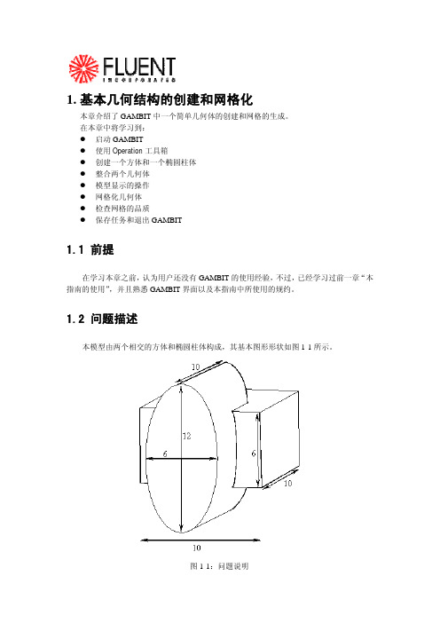
1.2 问题描述本模型由两个相交的方体和椭圆柱体构成,其基本图形形状如图1-1所示。
图1-1:问题说明1.3策略本章介绍使用GAMBIT生成网格的基本操作,特别地,将介绍:z如何使用“top-down”固体建模方法来方便地创建几何体z如何自动生成六面体网格“top-down”方法的意思是用户可以通过生成几何体(如方体、柱体等)来创建几何结构,然后,对它们进行布尔操作(如整合、剪除等),以这种方式,用户不用首先去创建作为基础的点、边和面,就可以快速创建出复杂的几何形体。
一旦创建出一个有效的几何模型,网格就可以直接并且自动地(很多情况下)生成。
在本例子中,将采用Cooper网格化算法来自动生成非结构化的六面体网格。
更复杂的几何结构在生成网格之前可能还需要进行手工分解,这将在后面进行介绍。
本章的学习步骤如下:z创建两个几何体(一个方体和一个椭圆柱体)z整合两个几何体z自动生成网格z检查网格的品质为了使本章的介绍尽量简短,一些必要的步骤被省略了:z调节几何体单边上节点的分布z设置连续介质类型(例如,标识哪些网格区是流体,哪些网格区是固体)和边界类型这些方面的详细内容,也包括其他方面,在随后的章节将涉及到。
1.4步骤输入gambit -id basgeom启动GAMBIT。
这就打开了GAMBIT的图形用户界面(GUI)(图1-2)。
GAMBIT把设定的名称(本例子中为basgeom)作为她将创建的所有文件的词头,如:basgeom.jou。
GAMBIT建模教程_附录B——GAMBIT中间文件格式

附录 B——GAMBIT 中间文件格式
GAMBIT 中间文件为 ASCII 文件,它可以用于导入或者导出网格数据,边界条件数据 (用名称识别的点、线或者表面)或者以节点或者单元基础格式的计算结果数据。以下部分 将详细说明 GAMBIT 中间文件的格式。 (注意:所有记录的数据格式都是根据 Fortran 规则 来表达的。 )
变量
NUMNP NELEM NGRPS NBSETS NDFCD NDFVL
说明
网格中的节点总数 网格单元总数 单元组数目 边界条件设置数目 坐标方向数目(2 或者 3) 速度份量数目(2 或者 3)
2
PDF 文件使用 "pdfFactory Pro" 试用版本创建
记录 2——计算器相关标识标题 格式:(3I10)
变量
NISOLV NRSOLV NSSOLV
说明
计算器相关整数值数目 解算器相关实数值数目 解算器相关字符串值数目
记录 3 到片断结尾——解算器相关标识 格式:( (8I10:)/(4E20.12:)/(A/))
变量
(ISOLVE(I),I=1,NISOLV) (RSOLVE(I),I=1,NRSOLV) (CSOLVE(I),I=1,NSSOLV)
单元连续性 这一部分包含单元连接性数据。 每个 NELEM 单元要有一个单独的数据记录, 因此本部 分包含 NELEM+2 个记录。 标题记录描述符 ELEMENTS/CELLS 记录 1 到 NELEM——节点坐标数据 格式:(I8,1X,I2,1X,I2,1X,7I8:/(15X,7I8:))
变量
变量
NGP NELGP MTYP
尺寸函数sizing-function

Tutorial:Introduction to Size FunctionsPurposeThe purpose of this tutorial is to introduce you to the use of size functions to control the size of mesh intervals for edges and mesh elements for faces and volumes.Based on their application,there are four types of size functions:fixed,curvature,proximity and meshed.This tutorial shows you how to use these size function types to refine a mesh in regions surrounding a specified entity and how to combine boundary layers and size functions for better mesh quality.PrerequisitesThis tutorial assumes that you are familiar with the GAMBIT interface and have a basic understanding of geometry creation and size functions.If you have not used size functions before,you can refer to Section5.2:Size Functions,in the GAMBIT Modeling Guide(http://www.fl/gambit2/doc/doc f.htm).Problem DescriptionYou will create a rectangular face,an elliptical cylindrical volume and a brick geometry and mesh them using the Fixed,Curvature,and Proximity size functions,respectively.Using a journalfile,you will then create and partially premesh2-D and3-D geometry.You will then use the meshed size function to grow the full mesh from the premeshed sections of the geometry.To create a size function,you need to define the Source and Attachment entities and param-eters such as,Growth rate,Size limit,Start size,Angle,and Cells/gap.The Growth rate and Size limit parameters are common to the four size functions.The additional parameter specific to three size functions,which is the initialization parameter used to create mesh on the source entities,is listed below:Type of Size Function Parameter Specific to the FunctionFixed Start sizeCurvature AngleProximity Cells/gapThe meshed size function does not require an initialization parameter,since we are starting from an existing mesh at the source entities.Introduction to Size FunctionsYou can specify more than one size function on any face or volume.Size functions can be used with hexahedral,tetrahedral or hybrid volume meshes and quadilateral or triangular face meshes.Since,you can control the number of elements in mapped or submapped meshes using edge grading,size functions are used in more complex geometries where tetrahedral or Cooper meshing schemes are required.Fixed Size FunctionThe Fixed size function is used to control the maximum mesh-element edge lengths in a model.Step1:Geometry1.Start GAMBIT with the identifier pipe.2.Create a rectangle with the following dimensions:Width Height10103.Create a circle with a value of Radius as1.4.Subtract the circle from the square.(a)In the Subtract Real Faces form,select face.1and face.2for Face and Subtract Facesrespectively.(b)Retain the default values of the other parameters and click Apply.5.Make two copies of the face and translate it.(a)In the Move/Copy Faces form,select face.1for Faces.(b)Select Copy and set the number of copies to2.(c)Under Global,set the value of x:to12.(d)Retain the default values of the other parameters and click Apply.Step2:Mesh the First Face1.Mesh the inner circular loop on thefirst face.(a)In the Mesh Edges form,for Edges,select the edge corresponding to the innercircular loop.(b)Set the Interval size to0.2and click Apply.2.Mesh thefirst face(see Figure1).(a)In the Mesh Faces form,select face.1for Faces and Tri for Elements:.(b)Retain the default values for the other parameters and click Apply.Introduction to Size FunctionsFigure1:Mesh on face.1Step3:Mesh the Second Face Using the Fixed Size Function1.Define afixed type function(fix1)on the second face(face.2).(a)On the Entities:Source:option button,select Edges and select the edge corre-sponding to the inner circular loop.(b)On the Entities:Attachment:option button,select the second face(face.2).(c)Set the values for the remaining parameters as follows:Start size Growth rate Size limit Label0.2 1.50.5fix12.Initialize the size function.(a)In the View Size Function form,selectfix1for S.Function and click Initialize.Note:The Iso-value:ranges from0.2to0.5.You can move the slider bar to examine the extent of the size function.The size function will not encompass the entireface.In the region excluded by the isovalues from0.2to0.5,the elements willhave a constant size of0.5.3.Mesh the second face.(a)Select face.2for Faces and Tri for Elements:.(b)Click Apply.The mesh obtained is muchfiner than the mesh on thefirst face because the valueof Size limit was specified as0.5.Introduction to Size Functions4.Delete the mesh on the second face.You will now adjust the size function parameters to get a coarser mesh on the secondface.5.Modify the size function(fix1)on the second face.(a)Change the value of Size limit to1and retain the default values of the otherparameters.6.Reinitialize the size function.Note:The Iso-value:now ranges from0.2to1.You can move the slider bar to examine the extent of the size function.The size function will not encompass theentire face.In the region excluded by the isovalues from0.2to1,the elementswill have a constant size of1.7.Remesh the second face(see Figure2).With the modified size function,you get a coarser mesh on the second face.Figure2:Mesh on face.2Step4:Mesh the Third Face Using the Fixed Size Function1.Define afixed type function(fix2)on the third face.(a)Set the Source:to the edge corresponding to the inner circular loop.(b)Set the Attachment:to face.3.(c)Set the values for the remaining parameters as follows:Start size Growth rate Size limit Label0.2 1.21fix2Introduction to Size Functions2.Initialize the size function.(a)In the View Size Function form,selectfix2for S.Function and click Initialize.Note:The Iso-value:ranges from0.2to1.You can move the slider bar to examine the extent of the size function.The size function will encompass the entire face.In the region excluded by the isovalues from0.2to1,the elements will have aconstant size of1.3.Mesh the third face with Tri elements.Figure3:Mesh on face.3You can compare the meshes shown in Figures1,2,and3.All the three meshes have the same mesh sizes on the edges,but the meshes created using a size function have a prescribed growth rate that results in fewer elements.Introduction to Size FunctionsCurvature Size FunctionThe Curvature size function controls the angles between the normals for adjacent mesh ele-ments and is useful when the model contains highly curved surfaces.Step1:Geometry1.Delete the previously created faces(face.1,face.2,and face.3).2.Create an elliptical cylinder with the following parameters:Height Radius1Radius2Axis Location1025Centered Z3.Make two copies of the elliptical cylinder and translate them.(a)In the Move/Copy Volumes form,select volume.1for Volumes and set the numberof copies to2.(b)Under Global,set the value of y:to12and x:and z:to0.(c)Retain the default values of the other parameters and click Apply.Step2:Mesh the First Volume1.In the Mesh Volumes form,select volume.1for Volumes and Tet/Hybrid for Elements:.2.Set the Interval size to2and click Apply.Figure4:Mesh on volume.1The mesh poorly represents the model in the regions where the edges are highly curvedand the surfaces are non planar.Introduction to Size Functions Step3:Mesh the Second Volume Using the Curvature Size Function1.Define a curvature type function(curv1).(a)Select Curvature for Type:.(b)On the Entities:Source:option button,select Faces and select the lateral face ofvolume.2.(c)On the Entities:Attachment:option button,select Volumes and select the volumeas volume.2.(d)Set the values for the remaining parameters as follows:Angle Growth rate Size limit Label40 1.22curv12.Mesh the second volume(volume.2)using tetrahedral elements.Figure5:Mesh on volume.2Now,the mesh is a much better approximation of the model where the regions are highly curved.Introduction to Size FunctionsStep4:Mesh the Third Volume Using the Curvature Size Function1.Define a curvature type function(curv2)on the third volume(volume.3).(a)Set the Source:to the lateral face of volume.3and the Attachment:to volume.3.(b)Change the value of Angle to20,and refer to the definition of curv1for values ofthe other parameters.2.Mesh the third volume(volume.3)using tetrahedral elements.Figure6:Mesh on volume.3pare the meshes for the second and third volume(see Figure7).The value of the angle determines the maximum angle between the normal vectors to adjacent mesh elements.Thus,a smaller angle(20degrees)will produce a better approximation toa curved edge than a larger angle(40degrees).Introduction to Size FunctionsFigure7:Magnified View of the Curved Edges of volume.3and volume.2Introduction to Size FunctionsProximity Size FunctionThe Proximity size function controls the number of mesh elements in faces between two geometric entities and is useful when there are small gaps in the model.Step1:Geometry1.Delete the previously created volumes(volume.1,volume.2and volume.3).2.Create a brick with the following dimensions:Width Depth Height Direction555Centered3.Create a thinner brick with the following dimensions:Width Depth Height Direction0.255Centered4.Move the thinner brick.(a)In the Move/Copy Volumes form,select volume.2or Volumes,and under Global,setthe values of x:to2,y:to0,and z:to2.5.5.Subtract the thinner brick from the larger brick.(a)In the Subtract Real Volumes form,select volume.1for Volume and volume.2forSubtract Volumes and click Apply.Figure8:Subtracted Volume(volume.1)There is a thin rectangular face(face.11)and a small gap of0.4width within thevolume bounded by the faces,face.13and face.1.6.Make a copy of the volume and translate it.(a)In the Move/Copy Volumes form,select volume.1for Volumes and set the numberof copies to1.(b)Under Global,set the value of x:to6,and y:and z:to0.(c)Retain the default values of the other parameters and click Apply.Step2:Mesh the First Volume Using Proximity Size Function1.Define a proximity type function(prox1)on thefirst volume(volume.1).(a)Select Proximity for Type:.(b)On the Entities:Source:option button,select Faces and select the thin rectangularface(face.11)of volume.1.(c)On the Entities:Attachment:option button,select Volumes and select the volumeas volume.1.(d)Set the values for the remaining parameters as follows:Cells/gap Growth rate Size limit Label3 1.31prox12.Mesh volume.1using tetrahedral elements.Figure9:Mesh on volume.1Figure10:Magnified View of Mesh on volume.1There are3elements in the thin rectangular face(face.11),however there is only one element in the thin gap bounded by the faces,face.13and face.1.Step3:Mesh the Second Volume Using Proximity Size Function1.Define a proximity function(prox2)on the second volume.(a)Set the Source:to the three faces(face.17,face.16,and face.25)of volume.2.(b)Set the Attachment:to volume.2,and refer to the definition of prox1for values ofthe other parameters.2.Mesh volume.2using tetrahedral elements.Now,there are3elements in the thin rectangular face(face.17)and three elements in the thin gap bounded by the faces,face.16,and face.25(see Figure12).Figure11:Mesh on volume.2Figure12:Magnified View of Mesh on volume.2Meshed Size FunctionThe meshed size function is used to grow mesh from source entities,which have been premeshed.This size function can be used for growing a graded surface mesh from pre-meshed edges or graded volume meshes from premeshed faces.You will need the journal file,meshed-sf-prep.jou for this section.Step1:Geometry and Premeshing using a Journal File1.Start GAMBIT with the identifier meshed-sf.2.In the File menu,select Run Journal....3.In the Run Journal form,select the Edit/Run mode.4.Click Browse...and navigate to the directory containing the journalfile meshed-sf-prep.jou.5.Select thefile meshed-sf-prep.jou and click Accept.6.In the Edit/Run Journal form,right-click the mouse and choose Select All in the drop-down menu.7.Click Step repeatedly to execute the commands in the journalfile one after another. Note:Observe the sequence of events on the screen from geometry creation to meshing ofedges and face.You may need to click the button to view all geometry.Step2:Mesh the First Face Using a Meshed Size Function1.Create a meshed size function with source as the edges and attachment entity asface.1.(a)Select Meshed as Type:.(b)On the Entities:Source:option button,select Edges and select all four premeshededges of thefirst face.(c)On the Entities:Attachment:option button,select thefirst face(face.1).(d)Set the values of the parameters as follows:Growth Rate Size Limit Label1.12meshed12.Mesh the face with quadrilaterals using the quad pave scheme.Figure13:Face Meshed Using Quad Pave SchemeIt can be observed that the mesh grows into the face from the edge meshes(Figure13).The face mesh can be made smoother orfiner by adjusting the growth rate and the size limit.This is useful for meshing complex faces containing edge meshes with different grading and spacing.Step3:Mesh the Volume Using a Meshed Size Function3.Create a meshed size function with source as the meshed face and attachment entityas volume.(a)Select Meshed as Type:.(b)On the Entities:Source:option button,select the Faces and select the premeshedface of the volume.(c)On the Entities:Attachment:option button,select Volume and select the volume(volume.1).(d)Set the values of the parameters as follows:Growth Rate Size Limit Label1.24meshed24.Mesh the volume with a Tet/Hybrid mesh using the Tgrid meshing scheme.Figure14:Cross-Sectional View of Mesh Along Length of the Volume It can be observed that the mesh grows from the premeshed face into the volume(Fig-ure14).The mesh can be changed by changing the growth rate and the size limit.This is useful in ensuring a smooth transition in mesh between different sections of a larger geometry or in growing a volume mesh from premeshed complex surfaces.In addition, the meshed sizing function can be used for creating a volume mesh grown from the end-capping surface of a prismatic boundary layer grown from surface meshes.Combining the Size Function and Boundary LayerSizing functions can also be combined with boundary layers.In the following example,the volume contains an interior void and the boundary layer must be attached to all the interior faces of this void.In this case,the internal continuity must be turned on.Step1:Geometry1.Delete the previously created volumes(volume.1and volume.2).2.Create a brick with the following dimensions:Width Depth Height Direction141414Centered3.Create an elliptical cylinder with the following parameters:Height Radius1Radius2Axis Location513Centered Z4.Subtract the cylinder from the brick.5.Make two copies of the subtracted volume and translate it.(a)Under Global,set the value of x:to16and y:and z:to0.Step2:Mesh the First Volume Using Size Functions1.Define a curvature type function curvbl1on thefirst volume(volume.1).(a)Select Curvature for Type:.(b)On the Entities:Source:option button,select Faces and select the lateral face ofthe cylinder.(c)On the Entities:Attachment:option button,select Volumes and select the volumeas volume.1.(d)Set the values for the remaining parameters as follows:Angle Growth rate Size limit Label30 1.31curvbl12.Mesh the volume using tetrahedral elements.3.Examine the mesh(see Figure15).(a)Set the Display Type:to Plane and select the tetrahedral3D Element.Figure15:Slice of the Mesh in the z directionStep3:Mesh the Second Volume Using Size Functions and Boundary Layer1.Define a curvature type function(curvbl2)on the second volume using the definitionfor curvbl1.2.Create a boundary layer for volume.2using the Uniform algorithm.(a)Set the values of the following parameters:First row Growth factor Rows0.2 1.23(b)Turn on Internal continuity.(c)Define the three faces(face.16,face.17,and face.18)of the cylinder as the At-tachment:.(d)Retain the default values for the other parameters and click Apply.3.Mesh the volume using tetrahedral elements.4.Examine the mesh.(a)Set the Display Type:to Plane and select the wedge3D Element.(b)Slide the slider bar in the Z direction(see Figure16).As you have used the uniform based boundary layer,you will see that the heightof thefirst layer of prism elements is constant.Figure16:Magnified View of the Prism Elements in the Boundary Layer(c)Select the tetrahedral3D Element and examine the growth of the elements out-wards from the interior void(see Figure17).Figure17:Slice of the mesh in the z directionStep4:Mesh the Third Volume Using Size Functions and Boundary Layer1.Define a curvature type function(curvbl3)on the third volume using the definition forcurvbl1.2.Create a boundary layer for volume.3using the Aspect ratio based algorithm.(a)Set the values of the following parameters:First percent Growth factor Rows30 1.23(b)Turn on Internal continuity.(c)Define the three faces(face.25,face.26,and face.27)of the cylinder as the At-tachment:.3.Mesh the volume using tetrahedral elements.4.Examine the mesh.(a)Set the Display Type:to Plane and select the wedge3D Element.(b)Slide the slider bar in the Z direction(see Figure18).Figure18:Magnified View of the Prism Elements in the Boundary LayerAs you have used the aspect ratio based boundary layer,you will see that theheight of thefirst layer of prism elements is not constant.Introduction to Size Functions(c)Select the tetrahedral3D Element and examine the growth of the elements out-wards from the interior void(see Figure19).Figure19:Slice of the Mesh in the z directionc Fluent Inc.June3,200521。
GAMBIT-几何操作

A B
– 相交体
B
A
A B
分离边
• 分离操作: 利用两个几何实体的相交部分去 把一个目标划分为两部分或划分多个目标 为多部分. • 把几何体分解为较小,较简单的单元体是 很有用的. • 边界分离
– 把一条边划分为多条边 – 产生的边默认为是连接的. – 边可以划分为:
• Point – 指定一个在 0 和 1之间的值为边将被 分离之处 – 用 0.5平分边. • 点 -一定是已经创建了的. • 边 – 一定是已经创建了的
– 所有面必须是平面
A B A
2 个面
B B A
• 相减体
B A B
多个实体可以输入到 第二个列表框中.
B A
A
2 个相交体
布尔操作 – 相交
• 实面/体布尔相交
– 选择的顺序不重要(除了 labeling) – 保留 – 保留复制的实体. – 所有的实体必须互相相交.
– 相交面 (所有面必须共面)
简单面
• 尺寸和平面/方向必须指定
– 矩形
– 圆
– 椭圆
体创建 – 面连接
• 能够创建一个或多个体通过连接一组面
– 对于一个单独的体, 如果一些面丢失了, Gห้องสมุดไป่ตู้MBIT能自动找到这些丢失的面. – 对于多个体, 任何多余的面都会被抛弃.
• 容差体缝合可以从在小容差内不相连的, 有缝隙的面创造单体
– 如果没有选上, 这些低层次的的几何体将 会保存下来
• 利用删除边/面/体来分离面和边.
• 一个实体如果它是从高层次命令实体引 用过来的,就不能被删除.
– 一个点属于一条边, 一条边 属于一个面,等等.
基本操作 – 混合
GAMBIT实例教程4_燃烧室模型的建立.
4. 燃烧室模型的建立(3-D )在这份指导书中,你可以通过运GAMBIT 中的top-down 几何结构法来为燃烧室生成几何模型(用实体来生成容积)。
你可以通过非结构化六面体网格法来为画出的燃烧室几何体划分网格。
在这份指导书中你可以学习到如何去:● 移动一个体积;● 从一个体积中扣除另一个;● 把一个体积阴影化;● 交叉两个体积;● 混合一个体积的边;● 通过对面进行扫描来生成体积;● 为读入FLUENT/UNS来准备网格。
4.1 前提这份指导书假定读者已经掌握了指导书1并且已对GAMBIT 界面相当熟悉。
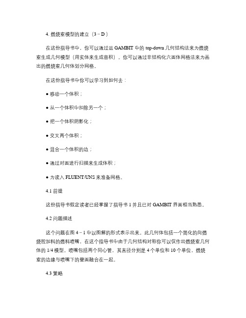
4.2 问题描述这个问题在图4-1中以图解的形式表示出来。
此几何体包括一个简化的向燃烧腔加料的燃料喷嘴,在这个指导书中由于几何结构对称你可以仅作出燃烧室几何体的1/4模型。
喷嘴包括两个同心管,其直径分别是4个单位和10个单位,燃烧室的边缘与喷嘴下的壁面融合在一起。
4.3 策略在这份指导书中,你可以运用top-down 几何结构法来生成燃烧室几何体,你可以生成体积(在本例中为方体和圆体)并用布尔运算把它们结合起来,交叉、扣除这些体积以生成基本体积,最后,通过“融和”命令,你可以舍掉一些边界以完成几何体生成。
在这个模型例子中,简单的选择捡起几何体并用六面体单元对整个区域进行网格划分是不可能的,由于Cooper 工具(在本向导中要应用)需要两组面,一组平行于扫描路径,另一组垂直于扫描路径,不管怎样,融和边界不适合于任一组。
对cooper 工具更详细的描述见GAMBIT Modeling Guide 。
你需要把几何体分成许能用cooper 来划分网格的部分。
在GAMBIT 中有许多分解几何体的方法。
在这个例子中,你可以采用把那些挨着弯面的体积部分从主体积中分开的方法。
对这个燃烧室进行分解的详细步骤在下面给出。
注意到几何体中有许多面,其默认的网格划分方案是pave 方案。
这些面中的大部分与Z 方向垂直。
gambit网格

3 模型的网格划分当用户点击Operation工具框中的Mesh命令按钮时,GAMBIT将打开Mesh子工具框。
Mesh子工具框包含的命令按钮允许用户对于包括边界层、边、面、体积和组进行网格划分操作。
与每个Mesh 子工具框命令设置相关的图标如下。
图标命令设置Boundary LayerEdgeFaceVolumeGroup3.1 边界层3.1.1 概述边界层确定在与边和/或者面紧邻的区域的网格节点的步长。
它们用于初步控制网格密度从而控制相交区域计算模型中有效信息的数量。
示例作为边界层应用的一个示例,考虑包括一个代表流体流过管内的圆柱的计算模型。
在正常环境下,很可能在紧靠管道壁面的区域内流体速度梯度很大,而靠近管路中心很小。
通过对壁面加入一个边界层,用户可以增大靠近壁面区域的网格密度并减小靠近圆柱中心的网格密度——从而获得表征两个区域的足够的信息而不过分的增大模型中网格节点的总数。
一般参数要确定一个边界层,用户必须设定以下信息:•边界层附着的边或者面•确定边界层方向的面或者体积•第一列网格单元的高度•确定接下来每一列单元高度的扩大因子•确定边界层厚度的总列数用户还可以设定生成过渡边界层——也就是说,边界层的网格节点类型随着每个后续层而变化。
如果用户设定了这样一个边界层,用户必须同时设定以下信息:•边界层过渡类型•过度的列数3.1.2 边界层命令命令详细说明图标Create Boundary Layer建立附着于一条边或者一个面上的边界层Modify Boundary Layer更改一个现有边界层的定义更改边界层标签Modify Boundary LayerLabelSummarize Boundary在图形窗口中显示现有边界层LayersDelete Boundary Layers删除边界层生成边界层Create Boundary Layer命令允许用户在一条边或者一个面附近定义网格节点步长。
要生成一个边界层,用户必须设定以下参数:•定义•过渡特性•附着实体和方向设定边界层定义要定一边界层,用户必须设定两类特征:•尺寸•内部连续性•角形状尺寸特征包括诸如边界层列数以及第一列高度等因数。
GMS中文使用手册

1.1.2 纲要......................................................................................................................................... 7
1.2 未安装 ESRI ARCOBJECTS............................................................................................................. 7 1.3 开始................................................................................................................................................ 7 1.4 读取 SHAPEFILE 文件..................................................................................................................... 7 1.5 查看 SHAPEFILE 文件..................................................................................................................... 8 1.6 查看属性表.................................................................................................................................... 8 1.7 文件转换为 2D 离散点..................................................................................................................9
- 1、下载文档前请自行甄别文档内容的完整性,平台不提供额外的编辑、内容补充、找答案等附加服务。
- 2、"仅部分预览"的文档,不可在线预览部分如存在完整性等问题,可反馈申请退款(可完整预览的文档不适用该条件!)。
- 3、如文档侵犯您的权益,请联系客服反馈,我们会尽快为您处理(人工客服工作时间:9:00-18:30)。
4. 设定区域类型
4.1 概述
区域类型设定确定了该区域截面和指定区域内的模型的实体和操作特征。
有两种典型的区域类型设定:
∙边界类型
∙连续介质类型
边界类型设定,例如WALL或者VENT,确定了模型的外部或者内部边界的特点。
连续介质类型,例如FLUID或者SOLID,确定了模型内部指定区域的特点。
以下部分强简要介绍边界类型和连续介质类型设定并结合包含简单几何结构的计算模型示例阐述它们定义的目的。
4.1.1 边界类型设定
边界类型设定确定了模型中那些代表模型边界的拓扑结构实体的物理特性和操作特性。
例如,如果用户将三维模型的一个面实体指定为INFLOW边界类型,该模型则被设定为介质从该设定面流入模型区域。
类似的,如果用户对于一个二维模型的边实体指定为SYMMETRY边界类型,则该模型被设定为流量、温度和压力梯度沿着指定边等于零。
因此,紧邻该边两侧的区域内的物理条件相同。
注意:要对于一个FLUENT解算器应用周期性边界条件,用户必须首先在应用边界条件的一组边(二维)或者一组面(三维)之间建立网格坚固连接。
(关于网格坚固连接的详细说明,参阅3.2.3部分。
)另外,用户必须为该组中的两条边或者两个面都设定PERIODIC 边界类型,并且这两条边(或者两个面)都必须作为一个单独实体的组成部分。
(如图4-1。
)
图4-1:周期性边界条件设定——FLUENT解算器
关于设定边界类型要求的步骤的完整说明,请参阅下面的4.2.1部分。
4.1.2 连续介质类型设定
连续介质类型设定确定模型你不指定区域的物理特性。
例如,如果用户对于一个体积实体指定了FLUID连续介质类型设定,该模型设定使得动量方程、连续性和网格节点和单元之间的物性传递存在于该体积中。
相反的,如果用户对于一个体积实体指定了SOLID连续介质类型,则仅仅有能量和物性传递方程(没有对流)将用用于该体积中现有的网格节点或者单元。
4.1.3 区域类型设定的影响
作为区域类型设定对于计算模型设定的影响的一个示例,考虑如图4-2所开始的几何结构——它包含一个直椭圆柱体。
该几何结构包含一个体积,三个面,两条边和两个顶点。
图4-2:边界和连续介质类型设定
如图4-2中所示的几何结构可以用于模拟很多不同类型的输运问题,包括流体通过一个直椭圆管路的流动和通过一个固体椭圆柱的导热。
表4-1和表4-2分别显示了与流体流动和导热问题有关的区域类型设定。
表4-1:流体流动问题区域类型设定
注意:计算计算器在它们使用边界类型和连续介质类型设定的方式上相互区别。
关于特定解算器应用边界类型设定和连续介质类型设定的说明,请查阅解算器文档。
4.2 区域命令
当用户点击Operation工具框中的Zones命令按钮时,GAMBIT将打开Zones子工具框。
该Zones子工具框中包含的命令按钮允许用户添加、更改和删除边界类型和连续介质类型设定以及撤销GAMBIT操作。
与每个Zones子工具框命令相关的图标如下。
本章的以下部分将详细说明上面列举的每个Zones命令。
4.2.1 设定边界类型
Specify Boundary Types命令允许用户对于代表模型边界的拓扑实体指定边界类型设定。
要建立边界类型设定,用户必须设定以下参数:
∙Name
∙Type
∙Entity集
Name参数是一个用来指定该设定的总体标签。
Type参数是一个代表物理或者操作特征的解算器特有关键字,例如WALL或者INFLOW。
Entity集由一个或者多个拓扑实体组成,Type 设定将应用于其上。
设定名称
当用户指定一个边界类型设定时,用户可以为该设定指定一个名称。
该名称作为该边界类型设定的总标签。
他可以浩瀚任意字母组合和/或者对于将读入该网格的解算器有效的
符号。
(注意:Polyflow解算器对于边界和连续介质名称具有特殊的限制。
特殊的,为Polyflow 解算器生成的网格的边界和连续介质名称必须遵守以下命名规则:
name.number
其中name为边界或者连续介质名称,number为顺序号。
例如,在一个给定模型中,边界实体可以指定为inflow.1,outflow.2和wall.3等名称。
)
设定类型
每个计算解算器与一系列允许的边界类型集合相关。
关于可用于每种GAMBIT支持的解算器的边界类型的详细说明,请查阅相应的解算器文档。
注意:如果用户在指定边界类型设定之后更改解算器,则GAMBIT将仅仅保留那些对于新的解算器有效的设定。
例如,如果用户选择了FIDAP解算器并指定WALL和SLIP边界类型设定,然后改为FLUENT/UNS解算器,GAMBIT将仅仅保留WALL边界类型设定——因为在FLUENT/UNS解算器中SLIP边界类型无效。
如果用户选择了FIDAP解算器,GAMBIT将重置前面FIDAP有效的边界类型设定以及对于FIDAP解算器有效的新的设定。
设定实体集合
每种边界类型设定必须包含一个实体集合。
该实体集合包括将应用Type设定的一个或者多个实体。
要在实体集合中添加一个实体,用户必须设定以下参数:
∙Type
∙Label
type参数确定要加入到该实体集合中的实体的类型。
label参数指要加入到该集合中的指定实体的名称。
指定实体类型
Specify Boundary Types窗口中的Entity部分中的选择按钮允许用户指定要加入到实体集合中的实体的一般类型。
对于边界类型设定有效的实体类型包括Edges、Faces和Groups。
如果用户选择了Groups选项,GAMBIT将在Entity列表框的右侧显示一个Edit命令按钮。
当用户点击Edit该按钮时,GAMBIT将打开Create Group窗口或者Modify Group窗口。
Create Group和Modify Group窗口分别允许用户建立或者修改一组实体,它们将包含在边界类型设定实体集合中。
(关于使用Create Group或者Modify Group窗口的详细说明,参阅本向导第二章。
)
注意:Specify Boundary Types窗口的Entity部分包含一个选择按钮和一个列表框,分别允许用户对于一个或者多个将要添加到实体集合中的实体指定类型和标签。
Entity部分也包含一个滑动列表,显示了当前存在于实体集合中的所有实体的Label和Type。
指定实体标签
要将一个实体添加到实体集合中,用户必须设定它的标签。
用户可以通过以下三种方式之一设定标签:
1.在Entity部分列表框中输入标签。
2.从相关的选择列表中选择标签。
3.使用鼠标在图形窗口中选择实体。
使用Specify Boundary Types窗口
要打开Specify Boundary Types窗口(如下图),点击Zones子工具框中的Specify Boundary Types命令按钮即可。
4.2.2 指定连续介质类型
Specify Continuum Types命令允许用户确定模型中任何由一组拓扑实体确定的区域的物理特性。
按顺序,物理特性将确定用于该问题的传输方程。
要建立连续介质类型设定,用户必须设定以下参数:
∙Name
∙Type
∙Entity集合
Name参数是指定该设定的一个总标签。
Type参数是一个代表物理或者操作特征的一个解算器特征关键字,例如WALL或者INFLOW Entity。
集合包含要应用Type设定的一个或者多个拓扑实体。
指定名称
(见上面的4.2.1对于连续介质类型Name参数的设定与上面的边界类型Name参数相同。
部分。
)
指定类型
有四种连续介质类型,每种类型与一组基本的迁移方程相关。
四种连续介质类型如下:∙FLUID
∙POROUS
∙SOLID
∙Conjugate (仅用于FLUENT 4)
注意:关于与连续介质类型相关的方程的详细说明,请查阅相应的解算器文档。
指定实体集合
连续介质类型集合的设定与上面边界类型的相似。
(见上面的4.2.1部分。
)它们的不同之处仅仅在于用户可以为Faces、Volumes和Groups指定的连续介质类型设定。
使用Specify Continuum Types窗口
要打开Specify Continuum Types窗口(如下图),点击Zones子工具框中的Specify Continuum Types命令按钮即可。
11。