Using Graphics Processing Units to Parallelize the FDK Algorithm for Tomographic Image Reconstru
硬件英语单词

硬件英文单词完全扫盲基本知识BGA(Ball Grid Array,球状矩阵排列)CMOS: Complementary Metal Oxide Semiconductor,互补金属氧化物半导体CISC(Complex Instruction Set Computing,复杂指令集计算机)COB(Cache on board,板上集成缓存)COD(Cache on Die,芯片内集成缓存)CPGA(Ceramic Pin Grid Array,陶瓷针型栅格阵列)CPU:Center Processing Unit,中央处理器EC(Embedded Controller,微型控制器)FEMMS:Fast Entry/Exit Multimedia State,快速进入/退出多媒体状态FIFO:First Input First Output,先入先出队列FPU:Float Point Unit,浮点运算单元HL-PBGA: 表面黏著,高耐热、轻薄型塑胶球状矩阵封装IA:Intel Architecture,英特尔架构ID:identify,鉴别号码IMM: Intel Mobile Module, 英特尔移动模块KNI(Katmai New Instructions,Katmai新指令集,即MMX2) MMX:MultiMedia Extensions,多媒体扩展指令集NI:Non-Intel,非英特尔PGA: Pin-Grid Array(引脚网格阵列),耗电大PSN(Processor Serial numbers,处理器序列号)PIB: Processor In a Box(盒装处理器)PPGA(Plastic Pin Grid Array,塑胶针状矩阵封装)PQFP(Plastic Quad Flat Package)RISC(Reduced Instruction Set Computing,精简指令集计算机) SEC: Single Edge Connector,单边连接器SIMD:Single Instruction Multiple Data,单指令多数据流SiO2F(Fluorided Silicon Oxide,二氧氟化硅)SOI: Silicon-on-insulator,绝缘体硅片SSE(Streaming SIMD Extensions,单一指令多数据流扩充) TCP: Tape Carrier Package(薄膜封装),发热小TLBs(Translate Look side Buffers,翻译旁视缓冲器) VLIW(Very Long Instruction Word,超长指令字) AGP: Accelarated Graphic Port(加速图形端口),一种CPU与图形芯片的总线结构APIC: Advanced Programmable Interrupt Controller(高级程序中断控制器)BGA: Ball Grid Array(球状网格阵列)BTB/C: Branch TargetBuffer/Cache (分支目标缓冲) CC: Companion Chip(同伴芯片),MediaGX系统的主板芯片组CISC: Complex Instruction Set Computing(复杂指令结构) CMOS: Complementary Metal Oxide Semiconductor(互补金属氧化物半导体)CP: Ceramic Package(陶瓷封装)CPGA: Ceramic Pin GridArray(陶瓷针脚网格阵列) CPU: Centerl Processing Unit(中央处理器)DCT: Display Compression Technology(显示压缩技术) DIB: Dual Independent Bus(双重独立总线),包括L2cache总线和PTMM(ProcesserTo Main Memory,CPU至主内存)总线DP: Dual Processing(双处理器) DX: 指包含数学协处理器的CPUECC: Error Check Correct(错误检查纠正)ECRS: Entry Call Return Stack(回叫堆栈),代替RAM存储返回地址.EPIC: Explicitly Parallel Instruction Computing(清晰平行指令计算),是一个64位指令集FPU: Floating-point Processing Unit(浮点处理单元)FRC: Functional Redundancy Checking (冗余功能检查,双处理器才有这项特性)IA: Intel Architecture(英特尔架构)I/ Input/Output(输入/输出)IS: Internal Stack(内置堆栈) ISO/MPEG: International Standard Organization's Moving Picture ExpertGroup(国际标准化组织的活动图片专家组)L1cache: Level1(一级)高速缓存,通常是集成在CPU中的,但现在也有把L2cache集成在CPU中的设计,如entium2LB: Linear Burst(线性突发),是Cyrix 6x86采用的特殊技术.MADD: 乘法-加法指令MAG: 乘法-累加指令,两浮点相乘后再和另一浮点数相加,可显著提高3D图形运算速度MHz: 工作频率的单位兆赫兹(Mega Hertz),1GHz=1000MHz MIPS: Million Instructions per Second(每秒钟百万条指令),是CPU速度的一个参数,当然是越大越好MMX: Multimedia Extensions(这个大家应该很熟悉了,这种CPU 有57新的64位指令,是自386以来的最大变化,另外还有SIMD架构等)MPGA: Micro PGA,散热和体积都比TCP小PGA: Pin Grid Array(引脚网格阵列),耗电大,适用用台式机pin: CPU的针脚PLL: Phase Lock Loop(阶段锁定) PR: P-rating,是一种额定性能指数,以Winstone 96测试为基本(PR2用Winstone97), 如PR-75即相当于奔腾75RISC: Reduced Instruction Set Computing(精简指令结构),是相对于CISC而言的ROB: Reorder Buffer(重新排序缓冲区)SC: Static Core(静态内核) SEC: Single Edge Contact(单边接触盒),是Intel的Pentium2CPU封装盒Slot 1: Pentium2的主板结构形式,外部总线频率66MHzSlot 2: Intel下一代芯片插座,处部总线频率达100MHz以上,有更大的SEC,主要用途是服务器,同时可安装4个CPUSMM: System Management Mode(系统管理模式),是一种节能模式Socket 7: 奔腾级(经典Pentium 和P55C)CPU的插座,外部总线频率83.3MHzSocket 8: 高能奔腾级CPU的插座,外部总线频率66MHz SP: Scratch Pad(高速暂存区) SRR: Segment RegisterRewrite(区段寄存器重写) SRAM: Static Random Access Memory(静态随机存储器) SUPER-7: 增加形Socket 7,外部总线频率100MHz,AGP,L2/L3cache,PC98,1 00MHzSDRAMSX: 指无数学协处理器的CPU TCP: Tape Carrier Package(薄膜封装),发热小,适用于笔记本式电脑.TLB: Translation Look side Buffer(翻译旁视缓冲器) VMA: Unified Memory Architecture(统一内存架构),系统内存和显示内存用Vcc2 为CPU内部磁心提供电压Vcc3(CLK) 为CPU的输入和输出信号提供电压VLIW: Very Long Instruction Word(极长指令字)VRE: V oltage Reduction Enhance(增强形电压调节) VSA: Virtual System Architecture(虚拟系统架构) Write-Back(写回): 是L1cache一种工作方式Write-Though(写通): 是L1cache 一种工作方式WHQL: Microsoft Windows Hardware Quality Lab(微软公司视窗硬件质量实验室)IEEE 1394---火线Firewire (IEEE-1394是在Windows98SE/2000/XP所支持的一种新标准的接口,其现有速率可达400Mbps,可显著提高多媒体视讯设备的传输速度,例如数码摄影机,扫描仪,打印机等等。
基于GPU_的多模式SAR_成像加速研究

第 21 卷 第 8 期2023 年 8 月Vol.21,No.8Aug.,2023太赫兹科学与电子信息学报Journal of Terahertz Science and Electronic Information Technology基于GPU的多模式SAR成像加速研究白澜1,3a,魏仁乐*2,3a,郭拯危3a,3b,3c,赵建辉3a,3b,3c,李宁3a,3b,3c(1.郑州科技学院信息工程学院,河南郑州450064;2.中共开封市委党校,河南开封475001;3.河南大学 a.计算机与信息工程学院;b.河南省大数据分析与处理重点实验室;c.河南省智能技术与应用工程技术研究中心,河南开封475004)摘要:针对多模式合成孔径雷达(SAR)成像处理中存在的计算效率不足问题,提出了一种基于GPU的多模式SAR统一成像并行加速方法。
为充分利用GPU的显存资源,提高算法的运算效率,利用共享内存对矩阵转置、矩阵相乘等部分进行大规模数据并行计算。
实验结果表明,该算法大幅度提升了多模式SAR成像的计算效率,最高加速比达到55.62,解决了GPU显存空间利用率较低的问题。
关键词:合成孔径雷达;图形处理器;多模式;并行加速中图分类号:TN958 文献标志码:A doi:10.11805/TKYDA2021142Multi-mode SAR imaging acceleration based on GPUBAI Lan1,3a,WEI Renle*2,3a,GUO Zhengwei3a,3b,3c,ZHAO Jianhui3a,3b,3c,LI Ning3a,3b,3c(1.College of Information Engineering,Zhengzhou Institute of Science and Technology,Zhengzhou Henan 450064,China;2.CPC Kaifeng Municipal Party School,Kaifeng Henan 475001;3a.College of Computer and Information Engineering;3b.Henan Key Laboratory of Big Data Analysis and Processing;3c.Henan Engineering Research Center of Intelligent Technologyand Application,Henan University,Kaifeng Henan 475004,China)AbstractAbstract::In view of the problem of low computational efficiency in multi-mode Synthetic Aperture Radar(SAR) imaging processing, a parallel acceleration method is proposed for multi-mode SAR imagingbased on Graphic Processing Unit(GPU). In order to make full use of GPU's memory resources andimprove the efficiency of the algorithm, in the parallel computing part of the algorithm, the large-scaledata parallel is carried out in the matrix transposition and matrix multiplication by using shared memory.The experimental results show that the algorithm greatly improves the efficiency of multi-mode SARimaging, and the maximum acceleration ratio reaches 55.62, which solves the problem of low utilizationof GPU.KeywordsKeywords::Synthetic Aperture Radar;Graphic Processing Unit;multi-mode;parallel acceleration合成孔径雷达(SAR)在军事和民生领域应用广泛。
IEEEtran_HOWTO

Please note that the appendices sections contain information on installing the IEEEtran class file as well as tips on how to avoid commonly made mistakes.
optional packages along with more complex usage techniques, can be found in bare_adv.tex.
It is assumed that the reader has at least a basic working knowledge of LATEX. Those so lacking are strongly encouraged to read some of the excellent literature on the subject [4]–[6]. In particular, Tobias Oetiker’s The Not So Short Introduction to LATEX 2ε [5], which provides a general overview of working with LATEX, and Stefan M. Moser’s How to Typeset Equations in LATEX [6], which focuses on the formatting of IEEE-style equations using IEEEtran’s IEEEeqnarray commands, are both available for free online.
CODE V 技术文档:如何准备模拟结果以进行演示、作业和其他出版物说明书
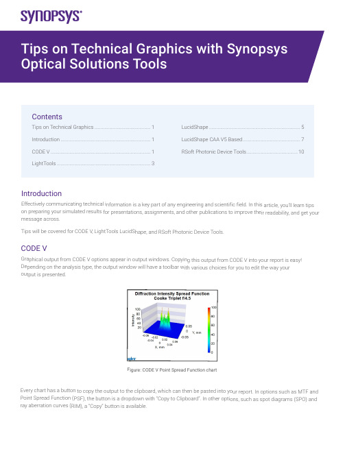
Introductio nEffectively com municating tec hnical informat ion is a key par t of any engine ering and scien tific field. In this article, you’ll le arn tips on preparing yo ur simulated re sults for presen tations, assignm ents, and other publications to improve their r eadability, and get your message acros s.Tips will be cov ered for CODE V, LightTools Lu cidShape, and R Soft Photonic D evice Tools.CODE VGraphical outp ut from CODE V options appea r in output wind ows. Copying t his output from CODE V into yo ur report is eas y! Depending on t he analysis typ e, the output w indow will have a toolbar with various choices for you to edit the way your output is presented.Figure: CODE V P oint Spread Func tion chartEvery chart has a button to cop y the output to the clipboard, w hich can then b e pasted into yo ur report. In op tions such as M TF and Point Spread F unction (PSF), t he button is a d ropdown with “Copy to Clipboa rd”. In other op tions, such as s pot diagrams (S PO) and ray aberration c urves (RIM), a “Copy” button is available.ContentsTips on Technical Graphics (1)Introduction (1)CODE V (1)LightTools ...........................................................................3LucidShape .........................................................................5LucidShape CAA V5 Based ..............................................7RSoft Photonic Device Tools .. (10)vFigure: Copying charts from CODE V’s MTF option and Spot Diagram optionAnalysis options such as MTF and PSF have buttons to increase font size and line width to aid you in making your output more legible when pasted into results. There is even an “Apply Presentation/Report Template” button to quickly prepare the chart for presentations:Figure: Controls to adjust chart font size, line width, and switch to “Apply Presentation/Report Template”Figure: MTF chart copied using the default MTF template (on left), and Presentation/Report settings (on right).Notice the text in the chart on the right is easier to read.For more extensive chart customizations, you can press the Chart Properties button to access controls for chart colors, axes scales, and more.Figure: Some options have a toolbar button to customize chart properties furtherRight click on the chart to save the property settings as a template to use later, or apply the settings to all similar charts in the window.Figure: Right clicking on a chart gives you options to apply and save templates,apply settings to all charts in the window, and revert settings back to the defaultFor charts that don’t have editable properties, such as spot diagrams and ray aberration curves, you can extract the components in Microsoft products and edit the picture:Figure: Copy of a RIM curve in Microsoft Powerpoint. Right click to edit the picture (left).Example of edited picture after adjusting font and line sizes (right)The edited picture becomes a Microsoft drawing object. These objects can then be ungrouped and moved/modified independently. LightToolsGraphical output from LightTools analysis can be accessed from the Analysis menu and choosing the metric you’d like to assess (illuminance, intensity, luminance, etc.). The main output is to present illumination metrics using the LumViewer, but there are also other types of analysis for color charts, polarization, and more. Each chart has a toolbar to help you customize how the analysis is presented.Copying charts from the LumViewer is easy! Right click on the copy icon and choose “Copy to Clipboard”. You can then paste the chart into your document.Figure: LumViewer’s “Copy to Clipboard”You can make text more readable by adjusting the font size up and down.Figure: In the LumViewer toolbar, you can adjust text font sizevFigure: Irradiance LumViewer plot copied with default settings (on left),compared to chart copied after increasing the font size to be more readible.For more extensive chart customizations, you can press the Chart Properties button to access controls for chart colors, axes scales, and more!Figure: Analysis options have a toolbar button to customize chart properties furtherRight click on the LumViewer to save the property settings as a template to use later, or apply the settings to all similar charts.Figure: Right clicking on a LumViewer chart gives you options to apply andsave templates and apply settings to all charts in the window.For luminance measurements, you can overlay forward simulation results directly on the associated geometry in the V3D window. To enable this setting, go to the View menu > Simulation Results and choose True Color or False Color.Figure: False color illuminance overlaid on lens geometry in the LightTools 3D ViewLucidShapeGraphical output from LucidShape can be customized from context menus for the specific output. After you’ve opened the results, you can customize the appearance by right clicking on the chart.Figure: Analysis from LucidShapeTo copy a chart or GeoView from LucidShape, right click in the window’s area and select “Copy Bitmap”. You can now paste the chart from the clipboard to the desired destination.Figure: To copy output from a chart or the GeoView, right click and choose “Copy Bitmap”You can use other options from the context sensitive menu as well. For example, when plotting sensor data you can switch ISO lines off for a smoother view, and select “View Properties” to open further chart customizations:Figure: For chart customization, right click and choose “View Properties”In the properties window, you can change settings such as the axes ranges, the type of chart, the scale, and more:Figure: The data properties windows lets you customize the way sensor data is presentedYou can customize the GeoView too! The context menu has choices to set the background color and edit the global axis system attributes the Stock Scene selection.• From the GeoView’s Options menu > GeoView, you can set the background color and edit stock sceneFigure: GeoView with the global axis system (on left) and without the stock scene visibleFrom the GeoView’s Options menu > Global Settings, you can increase the line widths to make wireframes clearer to see inpresentations and reports.Figure: Wireframe view with default width (on left) and increased line width (on right)The GeoView toolbar has options to change orientation and the change surface rendering mode. For instance, you can switch between shaded/wireframe modes, and even display sensor results from “Display Light Data”.Figure: GeoView with shaded geometry (on left), wireframe geometry (middle), and Display Light Data (on right) LucidShape CAA VA BasedTo take a screenshot in CATIA you can go to Tools > Image > Capture:Click the 3rd Icon “Options”:In the second tab “Pixel”, you can check “White background”, “Anti-aliasing” and switch render quality to “Highest”:Click OK, and back with these icons, click the second one “Select Mode”, and then do a left click, mode and release the left click in CATIA: a rectangle appears:By clicking the corners of the rectangle and moving them, you can resize the area which will be taken as screenshot.With the CATIA controls, you can move/rotate your design: the screenshot rectangle is not moving:Once the screenshot size is adjusted, click the first icon “Capture”: a new window is opening and you can either save the screenshot, or copy it:Also, in case you want to take a screenshot from the same viewing position, you may want to create cameras: in a product, go to Infrastructure > Photo Studio:vOn the right of the screen, click “Create camera” after you chose the view you needed:In the CATIA tree, under Applications, the camera is created. You also see a glyph in the 3D view. By double clicking the camera, you will look at your design always from the same view. With a right click, properties, you can move the camera:vRSoft Photonic Device ToolsAll RSoft Photonic Device Tools plot data through an included plotting program called WinPLOT. You can customize the plot through an editor with a comprehensive set of commands.Figure: A customized line plot (on left), and contour plot (on right) from RSoft WinPLOTCopying a plot from WinPLOT is easy, just go to the File menu > Export Graph to save to a variety of formats.Figure: Export RSoft WinPLOT plots from the File menu > Export GraphEach plot file contains a series of commands that control how the plot is displayed. Click the “View Editor” button in the toolbar to see and edit the commands. Then click the “View Plot” button to return to the plot. For example, the “/tt” command sets the “Title at the Top” of the plot. See the WinPLOT manual for command documentation.Figure: Edit WinPLOT settings from the View Editor• Learn more about using WinPLOT to create high-quality graphics for publications:–Line plots–Contour plotsVisit /optical-solutions to learn more about our optical design software tools, services, and equipment. Or contact us at ******************* so we can help you with demos, trial licenses, and product pricing.©2022 Synopsys, Inc. All rights reserved. Synopsys is a trademark of Synopsys, Inc. in the United States and other countries. A list of Synopsys trademarks isavailable at /copyright.html. All other names mentioned herein are trademarks or registered trademarks of their respective owners.03/23/22.tempfile_10000038.。
R Graphics画图经典教材-不得不看

Christoph Scherber, October 2007.
R Graphics ‐ October 2007 by Christoph Scherber (cscherb1@gwdg.de)
3
1. Standard plots
x<-c(1,3,4,6,8,9,12) y<-c(5,8,6,10,9,13,12)
(3) Some additional graphics features from interesting R libraries; examples are shown for barplots, 3D surface plots and for the display of meteorological data.
Y-Axis
12
10
8
10
12
X-Axis
There is a lot more to play around; here are some of the most useful graphics parameters from the par() command:
R Graphics ‐ October 2007 by Christoph Scherber (cscherb1@gwdg.de)
par(tck=0.02,las=1,cex.axis=1.3,b=1.2,mgp=c(3,0.5,0),bty ="L")
x<-c(1,3,4,6,8,9,12) y<-c(5,8,6,10,9,13,12) plot(x,y,type="n",axes=F,xlab="",ylab="") points(x,y,pch=16) axis(1) axis(2) title(xlab="X-Axis",ylab="Y-Axis") box()
(总结篇)使用MATLABGPU加速计算MATLAB并行计算与分布式服务器MATLAB技术论坛

(总结篇)使用MATLABGPU加速计算MATLAB并行计算与分布式服务器MATLAB技术论坛本帖最后由蓝云风翼于 2013-12-18 17:28 编辑注:利用gpu加速有一下工具1.JACKET 可从帖子中寻找2.MATLAB a.并行计算工具箱 gpuArray,查看支持gpuArray的函数methods('gpuArray')b.已经支持GPU的一些工具箱c.使用mex方式 /thread-33511-1-1.htmld.使用产生ptx方法编写cuda kernel这些都可以通过help gpuArray查看,建议使用最新版本2013a 查看GPU是否支持gpuDevice命令3.GPUMAT帖子中找4. nvmex方式即cudawhitepaper可从帖子中直接下载/thread-20597-1-1.html/thread-25951-1-1.htmlSIMULINK :/forum.php?mod=viewthread&tid=27230目前,GPU在通用数值计算领域的应用已经越来越广泛,MATLAB通过以下几种方式支持GPU。
一、MATLAB内嵌GPU函数fft, filter,及linear algebra operations等。
二、内嵌工具箱支持GPU的函数: Communications System Toolbox, Neural Network Toolbox, Phased Array Systems Toolbox, and Signal Processing Toolbox (GPU support for signal processing algorithms)三、在MATLAB中接入CUDA kernel,通过PTX方式或者MEX方式。
Multiple GPUs在单机和计算集群上的使用通过MATLAB 的并行计算工具箱(PCT)及MATLAB分布式计算工具箱(MDCS)(matlab worker)一、PCT GPUArrayParallel Computing Toolbox 提供 GPUArray,这是一个具有多个关联函数的特殊数组类型,可让您直接从MATLAB 在启用CUDA 的 NVIDIA GPU 上执行计算。
ImageProcessing_Unit1_slides爱丁堡大学图像处理研究生课程课件

Image Processing - Unit 1
javier.escudero@
10
Institute for Digital Communications (IDCOM) – Image Processing
256 × 256 pixels 128 × 128 pixels
Fig. 1.6 in Petrou’s
Image Processing - Unit 1 javier.escudero@ 12
Institute for Digital Communications (IDCOM) – Image Processing
Institute for Digital Communications (IDCOM) – Image Processing
Unit 1 – Introduction to digital image processing
Dr Javier Escudero javier.escudero@ School of Engineering / University of Edinburgh
False contouring – Content effects
Fig. 1.6 in Petrou’s
Image Processing - Unit 1 javier.escudero@ 17
Institute for Digital Communications (IDCOM) – Image Processing
False contouring (I)
• Keeping the size of the image constant and reducing the number of grey levels (G=2m) produces false contouring • However, this effect depends on the contents of the image
par函数的用法

par {graphics}R Documentation Set or Query Graphical ParametersDescriptionpar can be used to set or query graphical parameters. Parameters can be set by specifying them as arguments to par in tag = value form, or by passing them as a list of tagged values.Usagepar(..., no.readonly = FALSE)<highlevel plot> (..., <tag> = <value>)Arguments...arguments in tag = value form, or a list of tagged values. The tags must come from the names of graphical parameters described in the ‘Graphical Parameters’ section.no.readonly logical; if TRUE and there are no other arguments, only parameters are returned which can be set by a subsequent par() call on the same device.DetailsEach device has its own set of graphical parameters. If the current device is the null device, par will open a new device before querying/setting parameters. (What device is controlled by options("device").)Parameters are queried by giving one or more character vectors of parameter names to par.par() (no arguments) or par(no.readonly = TRUE) is used to get all the graphical parameters (as a named list). Their names are currently taken from the unexported variable graphics:::.Pars.R.O. indicates read-only arguments: These may only be used in queries and cannot be set. ("cin", "cra", "csi", "cxy", "din" and "page" are always read-only.)Several parameters can only be set by a call to par():"ask","fig", "fin","lheight","mai", "mar", "mex", "mfcol", "mfrow", "mfg","new","oma", "omd", "omi","pin", "plt", "ps", "pty","usr","xlog", "ylog","ylbias"The remaining parameters can also be set as arguments (often via ...) to high-level plot functions such as plot.default, plot.window, points, lines, abline, axis, title, text, mtext, segments, symbols, arrows, polygon, rect, box, contour, filled.contour and image. Such settings will be active during the execution of the function, only. However, see the comments on bg, cex, col, lty, lwd and pch which may be taken as arguments to certain plot functions rather than as graphical parameters.The meaning of ‘character size’ is not well-defined: this is set up for the device taking pointsize into account but often not the actual font family in use. Internally the corresponding pars (cra, cin, cxy and csi) are used only to set the inter-line spacing used to convert mar and oma to physical margins. (The same inter-line spacing multiplied by lheight is used for multi-line strings in text and strheight.)Note that graphical parameters are suggestions: plotting functions and devices need not make use of them (and this is particularly true of non-default methods for e.g. plot).ValueWhen parameters are set, their previous values are returned in an invisible named list. Such a list can be passed as an argument to par to restore the parameter values. Use par(no.readonly = TRUE) for the full list of parameters that can be restored. However, restoring all of these is not wise: see the ‘Note’ section. When just one parameter is queried, the value of that parameter is returned as (atomic) vector. When two or more parameters are queried, their values are returned in a list, with the list names giving the parameters.Note the inconsistency: setting one parameter returns a list, but querying one parameter returns a vector.Graphical ParametersadjThe value of adj determines the way in which text strings are justified in text, mtext and title. A value of 0 produces left-justified text, 0.5 (the default) centered text and 1 right-justified text. (Any value in [0, 1] is allowed, and on most devices values outside that interval will also work.)Note that the adj argument of text also allows adj = c(x, y) for different adjustment in x- and y- directions. Note that whereas for text it refers to positioning of text about a point, for mtext and title it controls placement within the plot or device region.annIf set to FALSE, high-level plotting functions calling plot.default do not annotate the plots they produce with axis titles and overall titles. The default is to do annotation.asklogical. If TRUE (and the R session is interactive) the user is asked for input, before a new figure is drawn. As this applies to the device, it also affects output by packages grid and lattice. It can be set even on non-screen devices but may have no effect there.This not really a graphics parameter, and its use is deprecated in favour of devAskNewPage.bgThe color to be used for the background of the device region. When called from par() it also sets new = FALSE. See section ‘Color Specification’ for suitable values. For many devices the initial value is set from the bg argument of the device, and for the rest it is normally "white".Note that some graphics functions such as plot.default and points have an argument of this name with a different meaning.btyA character string which determined the type of box which is drawn about plots. If bty is one of "o" (the default), "l", "7", "c", "u", or "]" the resultingbox resembles the corresponding upper case letter. A value of "n" suppresses the box.cexA numerical value giving the amount by which plotting text and symbols should be magnified relative to the default. This starts as 1 when a device is opened,and is reset when the layout is changed, e.g. by setting mfrow.Note that some graphics functions such as plot.default have an argument of this name which multiplies this graphical parameter, and some functions such as points and text accept a vector of values which are recycled.cex.axisThe magnification to be used for axis annotation relative to the current setting of cex.bThe magnification to be used for x and y labels relative to the current setting of cex.cex.mainThe magnification to be used for main titles relative to the current setting of cex.cex.subThe magnification to be used for sub-titles relative to the current setting of cex.cinR.O.; character size (width, height) in inches. These are the same measurements as cra, expressed in different units.colA specification for the default plotting color. See section ‘Color Specification’.Some functions such as lines and text accept a vector of values which are recycled and may be interpreted slightly differently.col.axisThe color to be used for axis annotation. Defaults to "black".bThe color to be used for x and y labels. Defaults to "black".col.mainThe color to be used for plot main titles. Defaults to "black".col.subThe color to be used for plot sub-titles. Defaults to "black".craR.O.; size of default character (width, height) in ‘rasters’ (pixels). Some devices have no concept of pixels and so assume an arbitrary pixel size, usually 1/72 inch. These are the same measurements as cin, expressed in different units.crtA numerical value specifying (in degrees) how single characters should be rotated. It is unwise to expect values other than multiples of 90 to work. Comparewith srt which does string rotation.csiR.O.; height of (default-sized) characters in inches. The same as par("cin")[2].cxyR.O.; size of default character (width, height) in user coordinate units. par("cxy") is par("cin")/par("pin") scaled to user coordinates. Note that c(strwidth(ch), strheight(ch)) for a given string ch is usually much more precise.dinR.O.; the device dimensions, (width, height), in inches. See also dev.size, which is updated immediately when an on-screen device windows is re-sized.err(Unimplemented; R is silent when points outside the plot region are not plotted.) The degree of error reporting desired.familyThe name of a font family for drawing text. The maximum allowed length is 200 bytes. This name gets mapped by each graphics device to a device-specific font description. The default value is "" which means that the default device fonts will be used (and what those are should be listed on the help page for the device). Standard values are "serif", "sans" and "mono", and the Hershey font families are also available. (Devices may define others, and some devices will ignore this setting completely. Names starting with "Hershey" are treated specially and should only be used for the built-in Hershey font families.) This can be specified inline for text.fgThe color to be used for the foreground of plots. This is the default color used for things like axes and boxes around plots. When called from par() this also sets parameter col to the same value. See section ‘Color Specification’. A few devices have an argument to set the initial value, which is otherwise "black".figA numerical vector of the form c(x1, x2, y1, y2) which gives the (NDC) coordinates of the figure region in the display region of the device. If you setthis, unlike S, you start a new plot, so to add to an existing plot use new = TRUE as well.finThe figure region dimensions, (width, height), in inches. If you set this, unlike S, you start a new plot.fontAn integer which specifies which font to use for text. If possible, device drivers arrange so that 1 corresponds to plain text (the default), 2 to bold face, 3 to italic and 4 to bold italic. Also, font 5 is expected to be the symbol font, in Adobe symbol encoding. On some devices font families can be selected by family to choose different sets of 5 fonts.font.axisThe font to be used for axis annotation.bThe font to be used for x and y labels.font.mainThe font to be used for plot main titles.font.subThe font to be used for plot sub-titles.labA numerical vector of the form c(x, y, len) which modifies the default way that axes are annotated. The values of x and y give the (approximate) numberof tickmarks on the x and y axes and len specifies the label length. The default is c(5, 5, 7). Note that this only affects the way the parameters xaxp and yaxp are set when the user coordinate system is set up, and is not consulted when axes are drawn. len is unimplemented in R.lasnumeric in {0,1,2,3}; the style of axis labels.0:always parallel to the axis [default],1:always horizontal,2:always perpendicular to the axis,3:always vertical.Also supported by mtext. Note that string/character rotation via argument srt to par does not affect the axis labels.lendThe line end style. This can be specified as an integer or string:and "round" mean rounded line caps [default];1and "butt" mean butt line caps;2and "square" mean square line caps.lheightThe line height multiplier. The height of a line of text (used to vertically space multi-line text) is found by multiplying the character height both by the current character expansion and by the line height multiplier. Default value is 1. Used in text and strheight.ljoinThe line join style. This can be specified as an integer or string:and "round" mean rounded line joins [default];1and "mitre" mean mitred line joins;2and "bevel" mean bevelled line joins.lmitreThe line mitre limit. This controls when mitred line joins are automatically converted into bevelled line joins. The value must be larger than 1 and the default is10. Not all devices will honour this setting.ltyThe line type. Line types can either be specified as an integer (0=blank, 1=solid (default), 2=dashed, 3=dotted, 4=dotdash, 5=longdash, 6=twodash) or as one of the character strings "blank", "solid", "dashed", "dotted", "dotdash", "longdash", or "twodash", where "blank" uses ‘invisible lines’ (i.e., does not draw them).Alternatively, a string of up to 8 characters (from c(1:9, "A":"F")) may be given, giving the length of line segments which are alternatively drawn and skipped. See section ‘Line T ype Specification’.Functions such as lines and segments accept a vector of values which are recycled.lwdThe line width, a positive number, defaulting to 1. The interpretation is device-specific, and some devices do not implement line widths less than one. (See the help on the device for details of the interpretation.)Functions such as lines and segments accept a vector of values which are recycled: in such uses lines corresponding to values NA or NaN are omitted.The interpretation of 0 is device-specific.maiA numerical vector of the form c(bottom, left, top, right) which gives the margin size specified in inches.marA numerical vector of the form c(bottom, left, top, right) which gives the number of lines of margin to be specified on the four sides of the plot.The default is c(5, 4, 4, 2) + 0.1.mexmex is a character size expansion factor which is used to describe coordinates in the margins of plots. Note that this does not change the font size, rather specifies the size of font (as a multiple of csi) used to convert between mar and mai, and between oma and omi.This starts as 1 when the device is opened, and is reset when the layout is changed (alongside resetting cex).mfcol, mfrowA vector of the form c(nr, nc). Subsequent figures will be drawn in an nr-by-nc array on the device by columns (mfcol), or rows (mfrow), respectively.In a layout with exactly two rows and columns the base value of "cex" is reduced by a factor of 0.83: if there are three or more of either rows or columns, the reduction factor is 0.66.Setting a layout resets the base value of cex and that of mex to 1.If either of these is queried it will give the current layout, so querying cannot tell you the order in which the array will be filled.Consider the alternatives, layout and split.screen.mfgA numerical vector of the form c(i, j) where i and j indicate which figure in an array of figures is to be drawn next (if setting) or is being drawn (ifenquiring). The array must already have been set by mfcol or mfrow.For compatibility with S, the form c(i, j, nr, nc) is also accepted, when nr and nc should be the current number of rows and number of columns.Mismatches will be ignored, with a warning.mgpThe margin line (in mex units) for the axis title, axis labels and axis line. Note that mgp[1] affects title whereas mgp[2:3] affect axis. The default is c(3, 1, 0).mkhThe height in inches of symbols to be drawn when the value of pch is an integer. Completely ignored in R.newlogical, defaulting to FALSE. If set to TRUE, the next high-level plotting command (actually plot.new) should not clean the frame before drawing as if it were on a new device. It is an error (ignored with a warning) to try to use new = TRUE on a device that does not currently contain a high-level plot.omaA vector of the form c(bottom, left, top, right) giving the size of the outer margins in lines of text.omdA vector of the form c(x1, x2, y1, y2) giving the region inside outer margins in NDC (= normalized device coordinates), i.e., as a fraction (in [0, 1]) ofthe device region.omiA vector of the form c(bottom, left, top, right) giving the size of the outer margins in inches.pageR.O.; A boolean value indicating whether the next call to plot.new is going to start a new page. This value may be FALSE if there are multiple figures on the page.pchEither an integer specifying a symbol or a single character to be used as the default in plotting points. See points for possible values and theirinterpretation. Note that only integers and single-character strings can be set as a graphics parameter (and not NA nor NULL).Some functions such as points accept a vector of values which are recycled.The current plot dimensions, (width, height), in inches.pltA vector of the form c(x1, x2, y1, y2) giving the coordinates of the plot region as fractions of the current figure region.psinteger; the point size of text (but not symbols). Unlike the pointsize argument of most devices, this does not change the relationship between mar and mai (nor oma and omi).What is meant by ‘point size’ is device-specific, but most devices mean a multiple of 1bp, that is 1/72 of an inch.ptyA character specifying the type of plot region to be used; "s" generates a square plotting region and "m" generates the maximal plotting region.smo(Unimplemented) a value which indicates how smooth circles and circular arcs should be.srtThe string rotation in degrees. See the comment about crt. Only supported by text.tckThe length of tick marks as a fraction of the smaller of the width or height of the plotting region. If tck >= 0.5 it is interpreted as a fraction of the relevant side, so if tck = 1 grid lines are drawn. The default setting (tck = NA) is to use tcl = -0.5.tclThe length of tick marks as a fraction of the height of a line of text. The default value is -0.5; setting tcl = NA sets tck = -0.01 which is S' default.usrA vector of the form c(x1, x2, y1, y2) giving the extremes of the user coordinates of the plotting region. When a logarithmic scale is in use (i.e.,par("xlog") is true, see below), then the x-limits will be 10 ^ par("usr")[1:2]. Similarly for the y-axis.xaxpA vector of the form c(x1, x2, n) giving the coordinates of the extreme tick marks and the number of intervals between tick-marks when par("xlog")is false. Otherwise, when log coordinates are active, the three values have a different meaning: For a small range, n is negative, and the ticks are as in the linear case, otherwise, n is in 1:3, specifying a case number, and x1 and x2 are the lowest and highest power of 10 inside the user coordinates, 10 ^ par("usr")[1:2]. (The "usr" coordinates are log10-transformed here!)n = 1will produce tick marks at 10^j for integer j,n = 2gives marks k 10^j with k in {1,5},n = 3gives marks k 10^j with k in {1,2,5}.See axTicks() for a pure R implementation of this.This parameter is reset when a user coordinate system is set up, for example by starting a new page or by calling plot.window or setting par("usr"): n is taken from par("lab"). It affects the default behaviour of subsequent calls to axis for sides 1 or 3.It is only relevant to default numeric axis systems, and not for example to dates.xaxsThe style of axis interval calculation to be used for the x-axis. Possible values are "r", "i", "e", "s", "d". The styles are generally controlled by the range of data or xlim, if given.Style "r" (regular) first extends the data range by 4 percent at each end and then finds an axis with pretty labels that fits within the extended range.Style "i" (internal) just finds an axis with pretty labels that fits within the original data range.Style "s" (standard) finds an axis with pretty labels within which the original data range fits.Style "e" (extended) is like style "s", except that it is also ensures that there is room for plotting symbols within the bounding box.Style "d" (direct) specifies that the current axis should be used on subsequent plots.(Only "r" and "i" styles have been implemented in R.)xaxtA character which specifies the x axis type. Specifying "n" suppresses plotting of the axis. The standard value is "s": for compatibility with S values "l"and "t" are accepted but are equivalent to "s": any value other than "n" implies plotting.xlogA logical value (see log in plot.default). If TRUE, a logarithmic scale is in use (e.g., after plot(*, log = "x")). For a new device, it defaults toFALSE, i.e., linear scale.A logical value or NA. If FALSE, all plotting is clipped to the plot region, if TRUE, all plotting is clipped to the figure region, and if NA, all plotting is clipped tothe device region. See also clip.yaxpA vector of the form c(y1, y2, n) giving the coordinates of the extreme tick marks and the number of intervals between tick-marks unless for logcoordinates, see xaxp above.yaxsThe style of axis interval calculation to be used for the y-axis. See xaxs above.yaxtA character which specifies the y axis type. Specifying "n" suppresses plotting.ylbiasA positive real value used in the positioning of text in the margins by axis and mtext. The default is in principle device-specific, but currently 0.2 for all ofR's own devices. Set this to 0.2 for compatibility with R < 2.14.0 on x11 and windows() devices.ylogA logical value; see xlog above.Color SpecificationColors can be specified in several different ways. The simplest way is with a character string giving the color name (e.g., "red"). A list of the possible colors can be obtained with the function colors. Alternatively, colors can be specified directly in terms of their RGB components with a string of the form "#RRGGBB" where each of the pairs RR, GG, BB consist of two hexadecimal digits giving a value in the range 00 to FF. Colors can also be specified by giving an index into a small table of colors, the palette: indices wrap round so with the default palette of size 8, 10 is the same as 2. This provides compatibility with S. Index 0 corresponds to the background color. Note that the palette (apart from 0 which is per-device) is a per-session setting.Negative integer colours are errors.Additionally, "transparent" is transparent, useful for filled areas (such as the background!), and just invisible for things like lines or text. In most circumstances (integer) NA is equivalent to "transparent" (but not for text and mtext).Semi-transparent colors are available for use on devices that support them.The functions rgb, hsv, hcl, gray and rainbow provide additional ways of generating colors.Line Type SpecificationLine types can either be specified by giving an index into a small built-in table of line types (1 = solid, 2 = dashed, etc, see lty above) or directly as the lengths of on/off stretches of line. This is done with a string of an even number (up to eight) of characters, namely non-zero (hexadecimal) digits which give the lengths in consecutive positions in the string. For example, the string "33" specifies three units on followed by three off and "3313" specifies three units on followed by three off followed by one on and finally three off. The ‘units’ here are (on most devices) proportional to lwd, and with lwd = 1 are in pixels or points or 1/96 inch.The five standard dash-dot line types (lty = 2:6) correspond to c("44", "13", "1343", "73", "2262").Note that NA is not a valid value for lty.NoteThe effect of restoring all the (settable) graphics parameters as in the examples is hard to predict if the device has been resized. Several of them are attempting to set the same things in different ways, and those last in the alphabet will win. In particular, the settings of mai, mar, pin, plt and pty interact, as do the outer margin settings, the figure layout and figure region size.ReferencesBecker, R. A., Chambers, J. M. and Wilks, A. R. (1988) The New S Language. Wadsworth & Brooks/Cole.Murrell, P. (2005) R Graphics. Chapman & Hall/CRC Press.See Alsoplot.default for some high-level plotting parameters; colors; clip; options for other setup parameters; graphic devices x11, postscript and setting up device regions by layout and split.screen.Examplesop <- par(mfrow = c(2, 2), # 2 x 2 pictures on one plotpty = "s") # square plotting region,# independent of device size## At end of plotting, reset to previous settings:par(op)## Alternatively,op <- par(no.readonly = TRUE) # the whole list of settable par's.## do lots of plotting and par(.) calls, then reset:par(op)## Note this is not in general good practicepar("ylog") # FALSEplot(1 : 12, log = "y")par("ylog") # TRUEplot(1:2, xaxs = "i") # 'inner axis' w/o extra spacepar(c("usr", "xaxp"))( nr.prof <-c(prof.pilots = 16, lawyers = 11, farmers = 10, salesmen = 9, physicians = 9, mechanics = 6, policemen = 6, managers = 6, engineers = 5, teachers = 4,housewives = 3, students = 3, armed.forces = 1))par(las = 3)barplot(rbind(nr.prof)) # R 0.63.2: shows alignment problempar(las = 0) # reset to defaultrequire(grDevices) # for gray## 'fg' use:plot(1:12, type = "b", main = "'fg' : axes, ticks and box in gray",fg = gray(0.7), bty = "7" , sub = R.version.string)ex <- function() {old.par <- par(no.readonly = TRUE) # all par settings which# could be changed.on.exit(par(old.par))## ...## ... do lots of par() settings and plots## ...invisible() #-- now, par(old.par) will be executed}ex()## Line typesshowLty <- function(ltys, xoff = 0, ...) {stopifnot((n <- length(ltys)) >= 1)op <- par(mar = rep(.5,4)); on.exit(par(op))plot(0:1, 0:1, type = "n", axes = FALSE, ann = FALSE)y <- (n:1)/(n+1)clty <- as.character(ltys)mytext <- function(x, y, txt)text(x, y, txt, adj = c(0, -.3), cex = 0.8, ...)abline(h = y, lty = ltys, ...); mytext(xoff, y, clty)y <- y - 1/(3*(n+1))abline(h = y, lty = ltys, lwd = 2, ...)mytext(1/8+xoff, y, paste(clty," lwd = 2"))}showLty(c("solid", "dashed", "dotted", "dotdash", "longdash", "twodash"))par(new = TRUE) # the same:showLty(c("solid", "44", "13", "1343", "73", "2262"), xoff = .2, col = 2) showLty(c("11", "22", "33", "44", "12", "13", "14", "21", "31"))[Package graphics version 3.4.0 Index]。