Schema Tutorial 4

合集下载

Gate4.0教程

●
●

Uses Xerxes-C XML parser (linux only)
●
Installation instructions included in example
15
Advanced Examples

HEP detectors
● ● ●
CMS hadron calorimeter test beam ATLAS Forward Liquid Ar Calorimeter LHCb Rich test beam

Toolkit Developers' Guide Physics Reference Manual Testing and Validation Demonstrating Geant4 tools Extending Geant4 Practical applications Examples from outside HEP (space, medical, etc.)
• Some were donated, and appear in Geant4
– G4TwistedTubs, G4Tet(rahedron), G4Ellipsoid, ..
Physics Reference Manual

URL: cern.ch/geant4/UserDocumentation/ UsersGuides/PhysicsReferenceManual/html/ PhysicsReferenceManual.html A reference for toolkit users and developers who wish to consult the underlying physics of an interaction Presents the theoretical formulation, model or parameterization of the physics interactions provided by Geant4

coot-tutorial

Coot TutorialCCP4School APS2010May20,2010Contents1Mousing2 2Introductory T utorial22.1Get theﬁles (2)2.2Start Coot (2)2.3Display Coordinates (2)2.4Adjust Virtual Trackball (3)2.5Display maps (4)2.6Zoom in and out (5)2.7Recentre on Different Atoms (5)2.8Change the Clipping(Slab) (7)2.9Recontour the Map (7)2.10Change the Map Colour (8)2.11Select a Map (8)3Model Building83.1Rotamers (8)3.2More Real Space Reﬁnement (9)4Blobology104.1Find Blobs (10)4.1.1Blob3 (10)4.1.2Blob2 (11)4.1.3Blob1 (12)5Extra Fun(if you have time)125.1Waters (12)5.2Working with NCS (13)5.3Add Terminal Residue (14)5.4Display Symmetry Atoms (15)5.5Skeletonization and Baton Building (16)5.6Reﬁne with Refmac (16)6Use the EDS166.1Make a(Pretty?)Picture (17)1MousingFirst,how do we move around and select things?Left-mouse Drag Rotate viewCtrl Left-Mouse Drag Translates viewShift Left-Mouse Label AtomRight-Mouse Drag Zoom in and outMiddle-mouse Centre on atomScroll-wheel Forward Increase map contour levelScroll-wheel Backward Decrease map contour level2Introductory T utorialIn this tutorial,we will learn how to do the following:1.Start Coot2.Display coordinates3.Display a map4.Zoom in and out5.Recentre on Different Atoms6.Change the Clipping(Slab)7.Recontour the Map8.Change the Map Colour9.Display rotamers and reﬁne residue2.1Get theﬁlesBefore we start,let’s get theﬁles on which we will be working:$wget /coot/tutorial/tutorial-modern.pdb$wget /coot/tutorial/rnasa-1.8-all refmac1.mtz or copy them from/home/emsley/tutorial2.2Start CootTo use coot,in a terminal window,type:$cootWhen youﬁrst start coot,it should look something like Figure1.2.3Display CoordinatesSo let’s read in those coordinates:•Select“File”from the Coot menu-bar11Note you can also use“Alt-F”instead of clicking on“File”Figure1:Coot at StartupNot much to see at present...Actually,after this,coot screenshots will bedisplayed with a white background,whereas you will see a black one•Select the“Open Coordinates”menu item[Coot displays a Coordinates File Selection window]•Either–Select tutorial-modern.pdb from the“Files”listor–Type tutorial-modern.pdb in the Selection:entry•Click“OK”in the Coordinates File Selection window[Coot displays the coordinates in the Graphics Window]2.4Adjust Virtual TrackballBy default,Coot has a“virtual trackball”to relate the motion of the molecule to the motion of the mouse.Many people don’t like this.So you might like to try the following.In the Coot main menu-bar:Edit→Preferences...[Coot displays a Preferences window]On the left toolbar select General and then on the right top notebook tab HID. Select“Flat”to change the mouse motion.(Use the“Spherical Surface”option to turn it back to how it is by default).What is the difference?“Flat”mode is like the mode used by“O”.In both modes,dragging the mouse near the centre of the screen causes the view to rotate about the X-or Y-axis.However in spherical mode you can also rotate about thez-axis by dragging the mouse along an edge of the window.Figure2:Coot After Loading Coordinates2.5Display mapsWe are at the stage where we are looking at the results of the reﬁnement.The reﬁnement programs stores its data(labelled lists of structure factor amplitudes and phases)in an“MTZ”ﬁle.Let’s take a look...•Select“File”from the Coot menu-bar•Select“Auto Open MTZ”menu item[Coot displays a Dataset File Selection window]•Select theﬁlename rnasa-1.8-all refmac1.mtzIf you choose instead“Open MTZ,cif or phs...”you will see:•[Coot displays a Dataset File Selection window]•Select theﬁlename rnasa-1.8-all refmac1.mtz[Coot displays a Dataset Column Label Selection window]Figure3:Coot MTZ Column Label Selection Window Notice that you have a selection of different column labels for the“Ampli-tudes”and“Phases”,however,let’s use the defaults:“FWT”and“PHWT”.•Press“OK”in the Column Label WindowNow open the MTZﬁle and select column labels“DELFWT”and“PHDELWT”.So now we have2maps(whether auto-opened or not).2.6Zoom in and outTo zoom in,click Right-mouse and drag it left-to-right2.To zoom out again,move the mouse the opposite way.Figure4:Coot after reading an MTZﬁle and zoomed in.2.7Recentre on Different Atoms•Select“Draw”from the Coot menu-bar•Select“Go T o Atom...”[Coot displays the Go To Atom window]•Expand the tree for the“A”chain•Select1ASP in the residue list•Click“Apply”in the Go To Atom window•At your leisure,use“Next Residue”and“Previous Residue”(or“Space”and “Shift”“Space”in the graphics window)to move along the chain.•Click Middle-mouse over an atom in the graphics window[Coot recentres on that atom]•Ctrl Left-mouse&Drag moves the view around.If this is a too slow and jerky:–Select Edit→Preferences...from Coot’s menu-bar–Select the“Maps”toolbutton on the left2or up-to-down,if you prefer that–Select the“Dragged Map”notebook tab.–Select“No”in the“Active Map on Dragging”window–Click“OK”in the“Preferences”windowNow the map is recontoured at the end of the drag,not at each step3.Another,additional way to make the movements faster is to change the num-ber of steps for the“Smooth Recentering”.Again youﬁnd this in the“Prefer-ences”(Preferences→General→Smooth Recentering).Change the“Num-ber of Steps”from the default80to something smaller,e.g.20.Figure5:Coot’s Go To Atom Window.•You can display the contacts too,as you do this:–Select“Measures”from the Coot menu-bar–Select“Environment Distances...”–Click on the“Show Residue Environment?”check-button∗Also Click“Label Atom?”if you wish the Cαatoms of the residuesto be labelled.–Click“OK”in the Environment Distances window–Click“Apply”in the Go To Atom window[You can’t change the colour of the Environment distances]You can turn off the Environment distances if you like.3which looks less good on faster computers.Figure6:Coot showing Atom Label and environment distances.2.8Change the Clipping(Slab)•Select“Draw”from the Coot menu-bar•Select“Clipping...”from the sub-menu[Coot displays a Clipping window]•Adjust the slider to the clipping of your choice•Click“OK”in the Clipping windowAlternatively,you can use“D”and“F”4on the keyboard,or Control Right-mouse up/down(Control Right-mouse left/right does z-translation).2.9Recontour the Map•Scroll your scroll-wheel forwards one click5[Coot recontours the map using a0.05electron/˚A3higher contour level]•Scroll your scroll-wheel forwards and backwards more notches and see the contour level changing.•If you don’t have a wheel on your mouse you can use“+”and“-”on the keyboard.•Note that the“Scroll”button in the Display Manager allows you to select which map is affected by this6.4think:Depth of Field.5don’t click it down.6by default it is the last map,which is not necessarily the map that you want.2.10Change the Map Colour•Select“Edit”from the Coot menu-bar•Select“Map Colour”in the sub-menu•Select“1xxx FWT PHWT”in the sub-menu[Coot displays a Map Colour Selection window]•Choose a new colour by clicking on the colour widgets[Coot changes the map colour to match the selection]•Click“OK”in the Map Colour Selection window2.11Select a MapSelect a map for model building:Menubar:Calculate→Model/Fit/Reﬁne...[Coot displays the Model/Fit/Reﬁne window]Select“Select Map...”from the Model/Fit/Reﬁne windowclick OK(you want to select the map with“...FWT PHWT”)Alternatively you can use the modelling toolbar icon buttons(here“Map”)dis-played on the right side of the Coot window.Most options found in the Model/Fit/Reﬁne window are available here too.If you are not sure which icon corresponds to which function look at the displayed tips when over the button with the mouse.Or change the display style of the buttons by clicking on the bottom arrow and select another style to get only or additionally text displayed.3Model Building“So what’s wrong with this structure?”you might ask.There are several ways to analyse structural problems and some of them are available in Coot.Validate→Density Fit Analysis→tutorial-modern.pdb[Coot displays a bar graph]Look at the graph.The bigger and redder the bar the worse the geometry.Thereare2area of outstanding badness in the A chain,around41A and89A.Let’s look at89Aﬁrst-click on the block for89A.[Coot moves the view so that89A CA is at the centre of the screen]3.1Rotamers•Examine the situation...[The sidechain is pointing the wrong way.Let’s Fix it...]•Menubar:Calculate→Model/Fit/Reﬁne (7)[Coot displays the Model/Fit/Reﬁne window]•Select“Rotamers”from the Model/Fit/Reﬁne window8.7or use the modelling toolbar on the right of the Coot window,i.e.you don’t need to open theModel/Fit/Reﬁne window8Or click on the“Rotamers”button of the modelling toolbar•In the graphics window,(left-mouse)click on an atom of residue89A(the Cγ,say)[Coot displays the“Select Rotamer”window]•Choose the Rotamer that most closely puts the atoms into the side-chain den-sity•Click“Accept”in the“Select Rotamer”window[Coot updates the coordinates to the selected rotamer]•Click“Real Space Reﬁne Zone”in the Model/Fit/Reﬁne window9.•In the graphics window,click on an atom of residue89A.Click it again.[Coot displays the reﬁned coordinates in white in the graphics and a new “Accept Reﬁnement”window]•Click“Accept”in the“Accept Reﬁnement”window.[Coot updates the coordinates to the reﬁned coordinates.89A nowﬁts the density nicely.]OK.That’s good.Now,how about if we just use Real Space Reﬁnement only?•Click“Undo”twice[Coot puts the sidechain back to the original position]•Click“Real Space Reﬁne Zone”in the Model/Fit/Reﬁne window10.•In the graphics window,click on an atom of residue89A.Click it again.[Coot displays the reﬁned coordinates in white in the graphics and a new “Accept Reﬁnement”window]•Now using left-mouse,click and drag on the intermediate(white)CZ atom of the PHE(if you mis-click the atom,the view will rotate).•Can you pull the atom around so that the side-chainﬁts the density?[Yes,you can]3.2More Real Space ReﬁnementNow let’s have a look at the other region of outstanding badness:•Click on the graph block for41A[Coot moves the view so that41A CA is at the centre of the screen]•Examine the situation...•Residue41is in a mess and notﬁtting to the density.Can youﬁx it?[Yes,you can]•The trick is Real Space Reﬁne that zone.So...9...or use the modelling toolbar button10...or modelling toolbar buttonFigure7:89A nowﬁts the density nicely.•You can either Real Space Reﬁne a few residues(40,41and42)or just41.Take your pick.•Click on“Real Space Reﬁne Zone”in the Model/Fit/Reﬁne window•Select a range by clicking on atoms in the graphics window(either atoms in 40then42or an atom in41twice)[Coot displays intermediate(white)atoms]•Click and drag on some atoms until the atomsﬁt nicely in the density.If you want to move a single atom then Ctrl Left-mouse to pick and move(just) that intermediate atom.[Note:Selecting and moving just the Carbonyl Oxygen is a good idea-use Ctrl Left-mouse to move just one atom.]4Blobology4.1Find BlobsTo be found under Validate(called“Unmodelled Blobs”).You can use the defaults in the subsequent pop-up.Press“Find Blobs”and wait a short while.You will get a new window that tell you that it has found unexplaned blobs. Time toﬁnd out what they are.4.1.1Blob3Let’s start from Blob3(the blobs are ordered biggest to smallest-Blobs3and4(if you have it)are the smallest).•Click on“Blob3”[Coot centres the screen on a blob]•Examine the situation...[We need something tetrahedral there...]•“Place Atom At Pointer”on the Model/Fit/Reﬁne window11[Coot shows a Pointer Atom Type window]•“SO4”in the new window...•In the“Pointer Atom Added to Molecule:”frame,change“New Molecule”to‘‘tutorial-modern.pdb”•Click OK.•Examine the situation...•the orientation is not quite right.•Let’s Real Space Reﬁne it(you should know what to do by now...)•(“Real Space Reﬁne Zone”then click an atom in the SO4twice.Accept)[The SO4ﬁts better now].Blob4is like Blob3(isn’t it?)4.1.2Blob2Click on the button“Blob2”and examine the density.Something is missing from the model.What?This protein and has been co-crystallized with its ligand substrate.That’s what missing:3’GMP.So let’s add it...•File→Get Monomer...•Type3GP in the box(Use Upper Case).Press return...[Coot pauses for a few seconds while LIBCHECK and REFMAC run][3GP appears]It is generally easier to work without hydrogens,so let’s delete them•“Delete...”from the Model/Fit/Reﬁne window12•“Hydrogens in Residue”•click on an atom in3GP[Hydrogens disappear]The3GP is displaced from where we want it to be.•“Rotate/T ranslate Zone”from the Model/Fit/Reﬁne window13•click on an atom in3GP twice[Intermediate(white)atoms appear]•Drag it or use the sliders to move the intermediate fragment to the approxi-mately the right place.11also available in the modelling toolbar12Found in the modelling toolbar?Of course!13Found it in the modelling toolbar?•Click“OK”in the slider window•Now optimize theﬁt using“Real Space Reﬁne Zone”like we did before.Now merge this ligand into the protein:•Calculate→Merge Molecules...•Click(activate)“monomer-3GP.pdb”•into Molecule:tutorial-modern.pdb•Merge4.1.3Blob1•Click on“Blob1”•Examine the situation...What is this density?[We need to add residues to the C-terminus of the A chain.]The missing residues are GLU,THR,CYS(QTC).•Calculate→Fit Loop...[Coot pops-ups a Fit Loop dialog]Add residue number94to96in the A chain.The single letter codes of the extra residues are QTC•Make sure that you can see the unmodelled density well,then click“Fit Loop”•Watch...(fun eh?)•Examine the densityﬁt.[It should beﬁne,except at the C-terminus.We need to add an OXT atom to the residue]•Calculate→Other Modelling T ools...•Add OXT to Residue...•Add it——————————————————This is a far as I expect you to get.——————————————————5Extra Fun(if you have time)5.1WatersFit waters to the structure•“Find Waters...”in the Other Modelling Tools dialog14,then OK(using the defaults)[Waters appear]14In older versions of Coot,the Find Waters button can be found in the Model/Fit/Reﬁne dialog or the water drop in the modelling toolbarTo check the waters:•Click on“Measures”in the main menubar.•Click on Environment Distances•Click on the“Show Residue Environment?”check-button•Change the distances as you like•Use the Go To Atom widget to go to theﬁrst water(probably towards the end of the list of residues in Chain“W”)•Use the Spacebar to navigate to the next residue(and Shift Spacebar to go backwards)•If you don’t like the fast sliding15you can turn it off(if you haven’t done so already):–Click Edit→Preferences...in the main menubar–Click General→“Smooth Recentering...”–Click“No”5.2Working with NCSThe tutorial data has two-fold NCS.With good data it is interesting to investigate the differences between the NCS copies.This may be done by comparing the NCS related electron density,comparing the NCS related chains,or comparing the Ra-machandran plots for related chains:•Comparing the NCS related electron density.Go to Calculate/NCS maps and select theﬁrst map and model.Now,if you go to anywhere in the A chain,you will see two sets of electron density-the original density for the A chain,and the density for the B chain transformed to overlap the A chain density.This gives you a visual comparison of any differences.Look at the density in the B molecule.Why does the density not agree here?(Hint:the NCS is not a2-fold rotation in this case,it is improper).•Comparing the NCS-related chains.Go to Draw/NCS ghost control and select Draw non-crystallographic ghosts.You will now see a copy of the B chain superimposed on the A chain.The B chain is draw using thin bonds.Look for regions where the models ing the NCS maps tool,check that the differences in the models are supported by the density.•Compare the NCS-related chains using“NCS jumping”.This is an alternative way of examining NCS similarities and e the Display Manager to undisplay the NCS maps you recently created above.Use the“Goto Atom”dialog and press the“Update from Current Position”button.[Coot shifts the centre of the screen to the closest displayed CA atom]15it’s not very good for water checkingIdentify the chain that you are looking at(for example,by double-clicking on an atom)Now press the“o”key on the keyboard.[Coot shifts the centre of the screen to a NCS-related chain]Identify the chain that you are looking at now.Press“o”again.What is happening?(Note:”o”stands for“Other NCS-related chain”.)•Comparing the Ramachandran plots for related chains.Go to Validate/Kleywegt plot.Check the Use speciﬁc chain options and select chains A and B.You will get a Ramachandran plot with equivalent residues from the A and B chains linked by arrows.Long arrows indicate signiﬁcant differences.Click on a dot to view the residue concerned.Another tool for identifying NCS differences is the Validate/NCS differences graph.This gives a clickable histogram of differences.5.3Add Terminal Residue[To be found on the Model/Fit/Reﬁne dialog16]•Use the Go To Atom window to go to residue72A.•What do you see?[You see missing atoms(that is,you don’t see them).This residue is supposed to bea CYS!Bad things have happened to it.Let’s get rid of this residue.][There may also be waters in the side-chain positions too(they have to be removed too).]•Delete...•(Make sure“Residue/Monomer”is active)•Click on an atom of residue72A.[Residue72A disappears]•Lets’put back an ALA.•Add Terminal Residue...[Coot adds intermediate white atoms and pops up a dialog]•Accept the new atomsOK,we now have a ALA.We want a CYS:•Mutate&Auto Fit...•Click on an atom in the new ALA[Coot pops up a residue type chooser]•Choose residue type CYS[Coot mutates andﬁts a CYS]16and in the modelling toolbar•Examine the situation.[There is an extra blob of density on that CYS.What is it?]It is an alternative conformation.Let’s model it•Add Alt Conf...[Coot pops up a residue splitter dialog]•Choose how you want to split your residue(the Right Way is an unresolved philosophical issue...17)•Click on an atom in72A[Coot adds intermediate white atoms and pops up a Rotamer Chooser]•Choose the correct rotamer-it shouldn’t be difﬁcult to tell which is the clos-est.•Accept when you are happy with you choice.•Now optimize theﬁt of this new residue with Real Space Reﬁnement.The reﬁnement of each alternate conformations is independent.•Real Space Reﬁne Zone•click on(say)SG,B of72A•Press“A”(on the keyboard)[Coot moves the atoms a bit]•Accept•Now do the same with the other conformation.[Ahhh!Much better.]5.4Display Symmetry AtomsTo be found on“Draw”→“Cell&Symmetry”menu item in the main menu.Try:•Show Symmetry Atoms?→Y es•Symmetry as Calphas?[on]•Colour symmetry by molecule[on]•Symmetry Radius30˚A•Colour Merge→0.1•Show Unit Cell?[on]•OK•Zoom out and have a look at how the molecules pack together.17Actually Jane Richardson may disagree with that statement.5.5Skeletonization and Baton BuildingYou can calculate the map skeleton in Coot directly:Calculate→Map Skeleton...→On.This can be used to“baton build”a map.You can turn off the coordinates and try it if you like(the Baton Building window can be found by clicking“Ca Baton Mode...”in the Other Modelling Tools dialog18).If you want to do this,I suggest you use Go To Atom and start residue2A(this allows you to build the complete A chain in the correct direction(it takes about15 minutes or so)and you can compare it to the real structure afterwards.Remember,when you start,you are placing a CA at the baton tip and at the start you are placing atom CA1.This might seem that you are“double-backing”on yourself-which can be confusing theﬁrst time.5.6Reﬁne with RefmacRefmac is a program that does Maximum Likelihood reﬁnement of the model,and the interface to it can be found on the Model/Fit/Reﬁne dialog.(By default there is no icon on the toolbar for this action-open the window from the calculate menu19). Now click on“Run Refmac...”(at the bottom of the Model/Fit/Reﬁne window).The defaults should beﬁne...“Run Refmac”in the new window......Wait...[The cycle continues...]•Use“Validate→Difference Map Peaks”toﬁnd interesting features in the newly created map and model.•Python enabled version only:a dialog with geometric outliers and other in-teresting things(if they exist)detected by Refmac shows up20.6Use the EDSLet’s validate a structure deposited in the PDB.Use a web browser and go to http://eds.bmc.uu.se/eds/.Use the keyword search toﬁnd the structure of a particular protein/ligand/author.File→Get PDB and Map Using EDSGet the accession code and paste it into the entry box that pops up.Use the validation tools in Coot to examine how good a PDBﬁle this is...[the Difference Map Peaks can be interesting]18this is quite advanced19or add your own“Run Refmac”button to the toolbar or the main/top toolbar.To add the button to the modelling/side toolbar,open the“Preference”window.Now go to Preferences→General→Reﬁnement T oolbar.In the right hand window scroll down and tick the box besides“Run Refmac...”.A corresponding button will appear on the modelling toolbar.Alternatively you can add your own “Run Refmac...”button to the top toolbar of the Coot window(only in Python versions).Click Right-mouse on the toolbar(besides the“Display Manager”button)and you will see a pop-up menu.Select “Manage Buttons”,tick the box besides“Add Alt Conf”and click“Apply”.A new button named“Add Alt Conf”will appear on the toolbar.20This is an analysis from the Refmac logﬁle and can alternatively be opened from Extensions...→Reﬁne...→Read REFMAC log6.1Make a(Pretty?)Picture(Depends on the appropriate supporting software being available):•Arrange a nice view•Press F8•Wait a few seconds...ColophonThis document is written using XEmacs21.5in L A T E X using AUCT E X and is dis-tributed with the Coot source code.。

Lecture_4

Nov-4-02 GAMIT/GLOBK Tutorial 4 9
autcln summary file
• One-way post-fit residual statistics – Only in postfit autcln summary – Gives RMS in mm
• by station and each satellite for a station • Normal values are 3-10 mm • >10 mm is not good
Nov-4-02 GAMIT/GLOBK Tutorial 4 5
Analyzing a solution: bias parameters
• Number of biases fixed – Fixed bias have no sigmas in Q-file – 608 B1L1 SMYC-TBLE 4- 2 0.0000000000 10.0000 \ – 609*B1L1 SMYC-TBLE 4- 5 0.0000000000 2.3133 \ 0.0367 -2.31330402 – The * means not fixed and sigma is given • Adjustments – parameters should not change much
Nov-4-02 GAMIT/GLOBK Tutorial 4 7
autcln output
• autcln.out.Z – full output – automatically compressed – use uncompress or use zcat to view – Lists actions taken by autcln • autcln.prefit.sum • autcln.post.sum – Summaries – Look at these

WaveDrom数字时序图渲染工具说明书

WaveDromRendering Beautiful Waveforms from Plain TextAliaksei ChapyzhenkaJonah ProbellAbstractWaveDrom is a tool for rendering digital timing diagrams, and other technical visualization, as SVG or PNG images from an intuitive plain text language. It is easy to learn, easy to use, and browser-based. WaveDrom is free open source software./This paper provides simple and complex examples of code and its resulting graphics. Also provided are guidelines on integrating WaveDrom into source code, diffing waveforms, parameterizing waveforms, describing and visualizing constraints, expressing design intent, and generating assertions.Table of ContentsIntroduction (3)Problems with current practices (3)Inspiration (4)Exchange format (WaveJSON) (5)Image rendering (5)Waveforms in code comments (8)Diffing waveforms (9)Parameterization (10)Representing constraints in WaveJSON (11)Generating assertions (13)Other users (16)Conclusion (16)IntroductionDigital t iming diagrams (“waveforms”) are the type of diagram that best describe how electronic signals do, or should, behave. Chip designers naturally draw waveforms on whiteboards, and routinely view waves when debugging simulations. When called upon to write a specification, we know our word processing options. However, there has never been a simple, widely used tool for rendering waveforms. That is until now.WaveDrom is a tool for rendering waveforms as SVG or PNG images.1 It defines a language that uses textual symbols, which are easy to create with a keyboard, to represent the types of information that waveforms present. WaveDrom follows the software development trend of running applications in browsers for automatic portability across operating systems. The WaveDrom editor (online and offline version) is WYSIWYG. The effect of changes to text describing waveforms is immediately rendered, without a compilation step. Furthermore, since WaveDrom waveforms are described as text, they can be embedded in source code comments, in source control metadata, and diffed between versions.WaveDrom was first created by this paper’s author, Aliaksei Chapyzhenka. It is available online, as desktop application (Windows, Linux, OSX), and open source on github.2 WaveDrom is well documented online with a fun interactive tutorial.3 Others have contributed ideas, and WaveDrom has been extended for:●drawing schematic diagrams●generating register field documentation● a translator to TikZ for TeX / LaTeX typesetting4This paper intends to stimulate ideas for other extensions and other uses.Problems with current practicesWaveforms are a common, well understood, industry standard way to express hardware behavior. When done well, they effectively communicate ideas visually, in a readable way.5Some readers of this paper draw waveforms as ASCII text. Some draw diagrams manually within a word processor’s graphics tools. Some copy-paste lines and hexagons in drawing programs. Some cleverly use cell outlining features in a spreadsheet, and some will even write Verilog with #delay 1 Scalable Vector Graphics (SVG) is a vector-based graphics format recognized by many document editing programs. Portable Network Graphics (PNG) is a raster graphics format, recognized by many document editing programs. PNG is comparable to the Joint Photographic Experts Group (JPEG) format.2https:///drom/wavedrom3 /tutorial4TikZ is a description format for vector graphics rendered in TeX and LaTeX documents. Describing timing diagrams in TikZ is not intuitive. See /tikz/examples/timing-diagram/.5 Tufte, Edward. Envisioning Information, 1990, andTufte, Edward. The Visual Display of Quantitative Information, 2001.statements, run a simulation with a trace file, and take screenshots of the traces in a waveform viewer GUI. Various commercial and freeware tools are available for download and installation on PCs to produce waveforms, but none is widely used.All such methods have important limitations:1.Not everyone is a visual artist, especially at work, and especially during routinework2.It takes time to make a good drawing3.Different authors draw with different and inconsistent styles4.Drawing waveforms directly intermingles presentation and content5.It is difficult to version control, change control, and compare waveforms6.Waveforms are not interactive7.It is difficult to assemble or concatenate multiple waveforms8.Waveforms are not parameterizedAs a result, designers avoid drawing waveforms where they could be helpful. When designers draw waveforms, they require editors and technical writers to redo the drawings for clarity. WaveDrom resolves all of these limitations. Furthermore, because WaveDrom uses a textual language it can serve as a modeling language that computers can parse. Designers at several companies use WaveDrom descriptions as part of hardware design entry, design capture, or test case entry. Furthermore, some designers parse simulation traces to generate WaveDrom waveforms for selected signals.InspirationThe concept of using textual (markup) language as a source for diagram rendering engine is not new. Many domain specific language exist to drive or hint diagram rendering process. There is full spectrum of language approaches.One approach is to provide some domain specific computer language that can be utilize standard computer language processing tools like lexer and parser, and processed than as abstract syntax tree. For example DOT to describe graphs or PlantUML to describe UML diagrams.Another approach is to employs the fact that block of monospace font text can have meaningful alignment that can be understood by the computer program. The ASCII graphics type descriptions like ditaa or shaape rely on fact of 2D alignment to render sophisticated block diagrams with desired spacial relationship of it’s parts, and certain color, shape, size effects.Some of the diagram languages employ standard mark languages (typically XML) to capture structure and content. For example: CML (Chemical Markup Language) For graphic rendering of the molecular structure of chemical compounds, or MathML (Mathematical Markup Language) to describe mathematical notations. JSON is new emerging standard for data object representation replacing XML in many areas.Exchange format (WaveJSON)WaveJSON is the compact exchange format used by WaveDrom to render waveforms.6 It is based on the JSON language syntax. WaveJSON is an Embedded Domain Specific Language.7 It uses the industry-standard JSON format with additional semantics embedded into the JavaScript object structure syntax.8WaveJSON satisfies the following criteria for a useful waveform exchange format:●Text format○Plain text editor can be used○Waveform code can be inserted into HDL or software code as comment○Code can be inserted into wiki, markdown, literate, or Asciidoctor documents9●Machine readable○JSON data object notation language○Has JSON schema: https:///wavedrom/wavedrom-schema that can be used for data validation.●Domain specific language (DSL)○Great expressive power within the domain○Exhibits minimum redundancy of domain specific knowledge definition○Is an extension of a general purpose language (i.e. JavaScript)●Open Source format and tools○WaveDrom : WaveJSON → SVG rendering engine in JavaScripthttps:///drom/wavedrom○WaveDromEditor : WaveJSON editor for Desktop and Browserhttps:///wavedrom/wavedrom.github.ioImage renderingThe first and most natural use for WaveDrom is rendering of images for publishing purposes.10 Here is a code example:6 The WaveJSON format specification is at https:///drom/wavedrom/wiki/WaveJSON7Mernik, Marjan, Jan Heering, and Anthony M. Sloane. "When and how to develop domain-specific languages." ACM computing surveys (CSUR) 37.4 (2005): 316-344.Knuth, Donald Ervin. The texbook. Vol. 1993. Reading, Massachusetts: Addison-Wesley, 1986.Spinellis, Diomidis. "Notable design patterns for domain-specific languages."Journal of systems and software 56.1 (2001): 91-99.8 JavaScript Object Notation (JSON) is an open standard format that uses human-readable text to transmit data objects consisting of attribute–value pairs. More information at /.9Knuth, Donald E. "Literate programming." CSLI Lecture Notes, Stanford, CA: Center for the Study of Language and Information (CSLI), 1992 1 (1992).Asciidoctor diagram extension at https:///asciidoctor/asciidoctor-diagram10 The online editor is available at /editor.html.The desktop application is available at https:///wavedrom/wavedrom.github.io/releases.{signal: [{wave: '01010101010101'}, // toggling{wave: '0.1.0.hl'}, // dot(.) holds a value, h/l for high and low {wave: '222xxx345.6789'}, // multi-bit, X, 345 = colors, 6789 == x{wave:''}, // blank line// text{wave: '2.2.2.2.2.2.2.',data:["abcdefg","hijk","lmnop","qrs","tuv","wx","yz"]},{wave:''},// names and clocks{name: "posclk", wave: 'pPp...........' }, // capital letters for arrows {name: "negclk", wave: 'n.N..n........' },{name: "divclk", wave: 'lplpl.h.l.h.pl' },{wave:''},// fun{name: "Barak", wave: '01.zx=ud.23.45'},// gaps{name: "gaps", wave: '01|022|0|x|.22' },// arrows with nodes and edges{name: "arrows", wave: '0n0....2..x2..',node: '.a........d' },{ wave: '1.0.10..x0....',node: '....b...c' },],edge:['a~>b glitch','c<~>d I found the bug!',],}It renders this waveform:The online tutorial has more examples and more sophisticated examples.WaveDrom render produces SVG or PNG. Standard skins can be used, but custom skins are supported for specific stylistic formatting. WaveDrom allows text to have XML style attributes.11 WaveDrom has a two panel editor that renders WaveJSON source into SVG image in realtime. The panels can be rotated to show the source and waveform horizontally or vertically. A user menu is in the lower right.11 Package available at https:///drom/tspanThe instant feedback of real time rendering gives a designer an ability to draw the intended waveform and correct mistakes very quickly.The following source code describes a DDR DRAM access:{ signal: [{ name: "CK", wave: "P.......", period: 2 },{ name: "CMD", wave: "x.3x=x4x=x=x=x=x",data: "RAS NOP CAS NOP NOP NOP NOP", phase: 0.5 },{ name: "ADDR", wave: "x.=x..=x........",data: "ROW COL", phase: 0.5 },{ name: "DQS", wave: "z.......0.1010z." },{ name: "DQ", wave: "z.........5555z.",data: "D0 D1 D2 D3" }]}Below is the rendered waveform.Waveforms in code commentsThe following Verilog module code includes a WaveDrom waveform in a code comment:module reducer(big, little)input [7:0] big;output [2:0] little;/* Waveform of example expected behavior{signal: [{name: 'big',wave: '=======',data: '0x0 0x1 0x5 0x10 0x3F 0x80 0xFF'},{name: 'little',wave: '=======',data: '0 0 3 4 5 7 7'},],}*/always @(*) beginlittle = 0;case(big)8’h02: little = 1;8’h04: little = 2;8’h08: little = 3;8’h10: little = 4;8’h20: little = 5;8’h40: little = 6;8’h80: little = 7;endcaseendendmoduleThe waveform code can be rendered for purposes of documentation. It would look like this.Diffing waveformsThough waveforms are the best way to display timing information in two dimensions, even when placed side by side it is very difficult to visually compare one to another to identify changes or differences. However, by representing waveforms as text, it is much easier to identify the difference between visual waveforms.Similarly, when a simulation or logic analyzer dumps a large amount of trace data as text, it is difficult to understand the diff in context. As long as the trace dump is in WaveDrom format, or can be easily converted to WaveDrom format by a script, then rendering the waveform as an image and looking at the point of the difference makes it much easier to understand.ParameterizationWaveDrom is built on JavaScript. Therefore, it is extensible. The example below is a waveform for a parameterizable memory block. It can return data in the same cycle, or with some latency. A JavaScript functions makes the read latency parameterizable, based on the variable rdlatency.(function (o) {var rdata = 'x.';rdata += '.'.repeat(o.rdlatency);rdata += '=..x';rdata += '.'.repeat(4 - o.rdlatency);return {signal: [{name: 'clk', wave: 'p.........'},{name: 'addr', wave: 'x=........', data: 'A<sub>0'},{name: 'rd', wave: '0.1..0....'},{name: 'rdata', wave: rdata, data: 'D<sub>0'}]};})({rdlatency: 1}) /* <-- change this */Representing constraints in WaveJSONWaveJSON has several features that can be used to describe behavioural constraints in the (human | computer) (readable | writable) language. Therefore, these features can facilitate human-machine interaction:●[signal[].wave] property represents one character per cycle, so it is possible to representalignment of several signals.●Vertical bar (|) character represents gaps in the timing.●[signal[].node] property allows placing anchors aligned with [signal[].wave] in time.●[edge] property describes dependencies between the nodes with optional textual attributes. Consider the following code.{signal: [{name: 'addr', wave: 'x=|', node: '.a..', data: 'a0'}, {},{name: 'ack', wave: '0.|1', node: '...b'},{name: 'data', wave: 'x.|=', node: '...c', data: 'd0'}],edge: ['a|->b [2:5]', 'b-c']}That yields the following waveform.Several system constraints can be drawn and analyzed from this description by human or computer. For example:1.one may expect ack to rise in 2 to 5 cycles after addr is asserted.2.The data signal should carry some payload, and be asserted on the same cycle.If the designer describes that expected behavior, then a computer can use it to:●Create a test case, and generate testbench code that behaves like the description, varyingparameters on the edges●Assert the constraint during simulation or for formal analysis●In the case of a mismatch (case failure), a computer can back-annotate the waveform,showing the difference with the actual behaviour, and use it for reporting.A report may contain multiple failing cases that look like this:{signal: [{name: 'addr', wave: 'x=x..', node: '.a..', data: '345'}, {},{name: 'ack', wave: '0.10.', node: '..b'}, {},{name: 'data', wave: 'x..=x', node: '...c', data: '825'}],edge: ['a--b expected [2:5] got 1', 'b--c expected 0 got 1'],head: {tock: 123}}rendered form:The report may have a timestamp or cycle number in a waveform header or footer section as a reference to the simulation time.Specific edges may contain more failure information.Below is code to represent a common protocol violation on an AMBA AXI read transaction.12 Text such as this could be generated by protocol checkers as part of verification IP packages:{ signal: [{ name: "CLK", wave: 'p..........', },{ name: "AR_VALID", wave: '01.0.......', },{ name: "AR_READY", wave: '0.10.......', },{ name: "AR_ADDR", wave: 'x=.x.......',data: "0x0000", },{ name: "R_VALID", wave: '0....1....0' },{ name: "R_READY", wave: '1.....01...',12 See /products/system-ip/amba-specifications.phpnode: '......a....', },{ name: "R_DATA", wave: 'x....====x.',data: "D0 D1 D2 D3",node: '.......b...', },],edge:['a~>b protocol violation: data change when READY is low'],}Below is the rendered waveform.Generating assertionsIt is possible for a user to express constraints using WaveJson in a way that they can both be rendered visually and translated, such as with a Perl script, into standard SystemVerilog assertions. There are an infinite number of ways to express constraints in WaveJson that make different trade-offs between readability and extensibility. Users should choose their format based on the range of types of assertions they intend to create, and what display format they find most readable.The authors of this paper are not recommending any particular syntax for assertion expression. Creating a script to perform a translation to SystemVerilog assertions is left as an exercise to the reader. Below are some possible examples.The following diagram is rendered from the following WaveDrom code (color added for emphasis).{ signal: [{name: 'REQ', wave: '010', node: '.ab'},{name: 'GNT', wave: '0|1', node: '..c'}],edge: ['a|>b ##[1]','a|>c ##[1:4]']}A simple translation of the WaveDrom code yields a property assertion for each edge such as the following SystemVerilog assertions.assert property (REQ |-> ##[1]~REQ); // a|bassert property (REQ |-> ##[1:4]GNT); // a|cThe translation uses the state, 1 or 0, of the wave corresponding to each node value to determine the state of the assertion implication (~ inversion). The translator uses SystemVerilog assertion syntax in the WaveDrom edge text. Other implementations could use any syntax appropriate for describing assertions. This opens a new level of assertion expression possibilities.In another example, the following WaveDrom code{signal: [{name: 'addr', wave: 'x=|', node: '.a..', data: 'a0'}, {},{name: 'ack', wave: '0.|1', node: '...b'},{name: 'data', wave: 'x.|=', node: '...c', data: 'd0'}],edge: ['a|->b ##[2:5]', 'b-c']}yieldsassert property (addr |-> ##[2:5]ack);assert property (ack |-> data);The rendered diagram looks like this.The dot character (‘.’) in WaveJson means repetition of the value of the previous cycle, which naturally maps to the SystemVerilog $stable construct.{ signal: [{ name: "READ", wave: "0.1..", node: '=.a..' },{ name: "DATA", wave: "=....", node: '=..b.' },],edge: ['a|->b']}One particular translation of the code above finds that the b node corresponds to a . in the DATA wave. Since the a node represents a transition to 1 in the READ wave, the following SystemVerilog assertion results.assert property (READ |=> $stable(DATA);The assertion waveform is rendered below.The translator converts the following WaveJson code{signal: [{name: 'full', wave: '1..', node: '.a..'},{name: 'write', wave: '1..', node: '.b..'},{name: 'read', wave: '0..', node: '.c..'},{name: 'wptr', wave: 'x=.', node: '..d.'},],edge: ['a&->d', 'b&->d', 'c&->d']}to the following SystemVerilog assertion./* full && write && !read |=> $stable(wptr) */Note that node d is the right hand side node for each edge, implying that the state of its signal (wptr) is the target of the assertion. The assertion waveform is rendered below.Other usersThe web version of WaveDrom is used by tens to hundreds of users at each of: Intel, AMD, Apple, Synopsys, Analog Devices, Nvidia, Cisco, National Semi, TI, ARM, Nvidia, HP, Marvell, Hynix, Infineon, Altera, Avago, Qualcomm, Volkswagen, Ford, and others.Many others outside of the semiconductor industry use or have adapted WaveDrom.Tutorial by Dave Vandenbout: /blog/timing-diagrams-made-easy/ Hackaday comparison to other waveform drawing applications:/2015/05/25/need-timing-diagrams-try-wavedrom/PSHDL Verilog coding game: /Yosys synthesis Verilog code verification game:http://www.clifford.at/yosys/nogit/YosysJS/snapshot/demo03.htmlCoroutine Co-simulation Test Bench (COCOTB) simulation trace to waveform usage:http://potential.ventures/beautiful-documentation.htmlBeagleBone BeagleLogic logic analyzer result display: http://beaglelogic.github.io/webapp/A simple function to add wavedrom waveforms into an ipython notebook:https:///witchard/ipython-wavedromA Trac plugin: https:///jun66j5/trac-wavedrompluginAsciidoctor Diagram extension: https:///asciidoctor/asciidoctor-diagramWhat will you do?ConclusionCurrent practices for drawing waveforms do not support a fast, easy, error-free workflow. WaveDrom does so with an intuitive plain text language for describing waveforms. A free, open source editor renders clear diagrams with a consistent format. WaveDrom text is easy to embed in source code comments. Furthermore, WaveDrom text allows for diffing waveforms. Waveforms can also be parameterized. Waveforms becomes a source for describing and for visualizing constraints. Edges within waveforms naturally indicate relationships, and can be translated to other expression syntaxes such as SystemVerilog assertions. A lot of companies already use WaveDrom in their design work. Shouldn’t you?。

BIEE最全的中文教程

1目录1 ORACLE BIEE基础 (4)1.1 OBIEE 概述 (4)1.1.1 BIEE 历史 (4)1.1.2 数据模型 (4)1.2 BIEE 安装 (5)1.2.1 JDK要求 (5)1.2.2 下载BIEE (6)1.2.3 安装BIEE (6)1.2.4 Logs (8)1.3 配置 (9)1.3.1 安装后的目录 (9)1.3.2 几个重要的配置文件 (9)1.4 预览Demo效果 (9)1.4.1 启动BI服务和OC4J (9)1.4.2 打开BIEE仪表盘 (10)2 BIEE 开发步骤 (12)2.1 数据库 (12)2.1.1 安装数据库 (12)2.2 创建资料库 (12)2.2.1 资料库 (12)2.3 创建物理模型 (13)2.3.1 导入物理表 (13)2.3.2 选择维度表和事实表 (14)2.3.3 完成物理模型 (15)2.3.4 新建主键和外键 (16)2.4 创建逻辑模型 (18)2.4.1 创建逻辑层 (18)2.4.2 查看逻辑层 (19)2.4.3 修改逻辑层 (19)2.5 创建展现模型 (20)2.5.1 创建展现层 (20)2.6 保存资料库 (21)2.6.1 保存资料库 (21)2.6.2 修改密码 (22)2.7 发布资料库 (22)2.7.1 修改NQSConfig.INI (22)2.7.2 重启Oracle BI Server (22)2.8 Answers –答复 (23)2.8.1 登陆BI Dashboards (23)2.8.2 选择主题 (23)2.8.4 新建文件夹 (25)2.8.5 保存报表 (26)2.9 Dashboards –仪表盘 (27)2.9.1 创建仪表盘 (27)2.9.2 编辑仪表盘 (27)2.9.3 查看仪表盘 (28)3 Answer详细介绍 (29)3.1 列 (29)3.1.1 新建报表 (29)3.1.2 列属性 (30)3.1.3 fx-编辑属性 (30)3.1.4 添加筛选器 (31)3.1.5 最终效果 (32)3.2 答复 (33)3.2.1 Prompts-报表提示 (33)3.2.2 Title-标题 (33)3.2.3 Legend-图例 (34)3.2.4 Narrative-叙述内容 (35)3.2.5 Ticker-标记视图 (36)3.2.6 合计 (37)3.2.7 Chart-图表 (38)3.2.8 Pivot Table-数据透视图 (39)3.2.9 Gauge-计量表 (39)3.2.10 Column Selector-列选择器 (41)3.2.11 View Selector-视图选择器 (41)4 Dashboard详细介绍 (43)4.1 仪表盘设置 (43)4.1.1 管理 (43)4.1.2 我的账户 (43)4.2 仪表盘功能 (43)4.2.1 Dashboard Prompt-仪表盘提示 (44)4.2.2 Link or Image-链接或图像 (44)4.2.3 Embedded Content-嵌入式内容 (45)4.2.4 Text-文本 (46)4.2.5 Briefing Book-简要簿 (47)4.2.6 Folder-文件夹 (49)4.2.7 Guided Nav. Link-引导导航链接 (49)4.2.8 Briefing Book Nav. Link-工作簿导航链接 (50)4.2.9 BI Publisher 报表 (51)4.2.10 条件显示内容 (51)5 Delivers介绍 (53)5.1 Scheduler 配置 (53)5.1.1 安装计划表 (53)5.1.3 添加用户认证 (55)5.1.4 查看Scheduler (56)5.2 Delivers应用 (57)5.2.1 编辑我的客户 (57)5.2.2 创建iBot (58)5.2.3 查看Alerts (60)5.2.4 发送Mail (60)6 其他功能介绍............................................................................................错误!未定义书签。

Neo4j教程：基础到高级概念说明书

About the T utorialNeo4j is one of the popular Graph Databases and Cypher Query Language (CQL). Neo4j is written in Java Language. This tutorial explains the basics of Neo4j, Java with Neo4j, and Spring DATA with Neo4j.The tutorial is divided into sections such as Neo4j Introduction, Neo4j CQL, Neo4j CQL Functions, Neo4j Admin, etc. Each of these sections contain related topics with simple and useful examples.AudienceThis tutorial has been prepared for beginners to help them understand the basic to advanced concepts of Neo4j. It will give you enough understanding on Neo4j from where you can take yourself to a higher level of expertise.PrerequisitesBefore proceeding with this tutorial, you should have basic knowledge of Database, Graph Theory, Java, and Spring Framework.Copyright & Disclaimer© Copyright 2018 by Tutorials Point (I) Pvt. Ltd.All the content and graphics published in this e-book are the property of Tutorials Point (I) Pvt. Ltd. The user of this e-book is prohibited to reuse, retain, copy, distribute or republish any contents or a part of contents of this e-book in any manner without written consent of the publisher.We strive to update the contents of our website and tutorials as timely and as precisely as possible, however, the contents may contain inaccuracies or errors. Tutorials Point (I) Pvt. Ltd. provides no guarantee regarding the accuracy, timeliness or completeness of our website or its contents including this tutorial. If you discover any errors on our website or in this tutorial, please notify us at **************************T able of ContentsAbout the Tutorial (i)Audience (i)Prerequisites (i)Copyright & Disclaimer (i)Table of Contents (ii)1.Neo4j ─ Overview (1)What is a Graph Database? (1)Advantages of Neo4j (2)Features of Neo4j (2)2.Neo4j ─ Data Model (4)3.Neo4j ─ Environment Setup (6)Neo4j Database Server Setup with Windows exe File (6)Starting the Server (9)Working with Neo4j (11)4.Neo4j ─ Building Blocks (12)Node (12)Properties (12)Relationships (13)Labels (14)Neo4j Data Browser (14)NEO4J ─ CQL (17)5.Neo4j CQL ─ I ntroduction (18)Neo4j CQL Clauses (18)Neo4j CQL Functions (20)Neo4j CQL Data Types (21)CQL Operators (21)Boolean Operators in Neo4j CQL (22)Comparison Operators in Neo4j CQL (22)6.Neo4j CQL ─ Creating Nodes (24)Creating a Single node (24)Creating Multiple Nodes (27)Creating a Node with a Label (30)Creating a Node with Multiple Labels (33)Create Node with Properties (36)Returning the Created Node (39)7.Neo4j CQL ─ Creating a Relationship (42)Creating Relationships (42)Creating a Relationship Between the Existing Nodes (44)Creating a Relationship with Label and Properties (47)Creating a Complete Path (49)N EO4J CQL ─ WRITE CLA USES (51)8.Neo4j ─ Merge Command (52)Merging a Node with a Label (52)Merging a Node with Properties (56)OnCreate and OnMatch (58)Merge a Relationship (61)9.Neo4j ─ Set Clause (63)Setting a Property (63)Removing a Property (65)Setting Multiple Properties (67)Setting a Label on a Node (69)Setting Multiple Labels on a Node (71)10.Neo4j ─ Delete Clause (74)Deleting All Nodes and Relationships (74)Deleting a Particular Node (75)11.Neo4j ─ Remove Clause (77)Removing a Property (77)Removing a Label From a Node (79)Removing Multiple Labels (81)12.Neo4j ─ Foreach Clause (84)NEO4J CQL ─ READ CLA USES (87)13.Neo4j ─ Match Clause (88)Get All Nodes Using Match (88)Getting All Nodes Under a Specific Label (90)Match by Relationship (92)Delete All Nodes (94)14.Neo4j ─ Optional Match Clause (96)15.Neo4j ─ Where Clause (98)WHERE Clause with Multiple Conditions (101)Using Relationship with Where Clause (103)16.Neo4j ─ Count Function (106)Count (106)Group Count (108)N EO4J CQL ─ GENERAL C LAUSES (111)17.Neo4j ─ Return Clause (112)Returning Nodes (112)Returning Multiple Nodes (114)Returning Relationships (116)Returning Properties (118)Returning All Elements (120)Returning a Variable With a Column Alias (122)18.Neo4j ─ Order By Clause (124)Ordering Nodes by Multiple Properties (126)Ordering Nodes by Descending Order (128)19.Neo4j ─ Limit Clause (131)Limit with expression (133)20.Neo4j ─ Skip Clause (136)Skip Using Expression (138)21.Neo4j ─ With Clause (140)22.Neo4j ─ Unwind Clause (142)NE O4J CQL ─ FUNCTIONS (144)23.Neo4J CQL ─ String Functions (145)String Functions List (145)Upper (145)Lower (147)Substring (149)24.Neo4j ─ Aggreg ation Function (152)AGGREGATION Functions List (152)COUNT (152)MAX (155)MIN (157)AVG (159)SUM (161)N EO4J CQL ─ ADMIN (163)25.Neo4j ─ Backup & Restore (164)Neo4j Database Backup (164)Neo4j Database Restore (171)26.Neo4j ─ Index (174)Creating an Index (174)Deleting an Index (176)27.Neo4j ─ Create Unique Constraint (179)Create UNIQUE Constraint (179)28.Neo4j ─ Drop Unique (182)Neo4j5Neo4j is the world's leading open source Graph Database which is developed using Java technology. It is highly scalable and schema free (NoSQL).What is a Graph Database?A graph is a pictorial representation of a set of objects where some pairs of objects are connected by links . It is composed of two elements - nodes (vertices) and relationships (edges).Graph database is a database used to model the data in the form of graph. In here, the nodes of a graph depict the entities while the relationships depict the association of these nodes. Popular Graph DatabasesNeo4j is a popular Graph Database. Other Graph Databases are Oracle NoSQL Database, OrientDB, HypherGraphDB, GraphBase, InfiniteGraph, and AllegroGraph.Why Graph Databases?Nowadays, most of the data exists in the form of the relationship between different objects and more often, the relationship between the data is more valuable than the data itself.Relational databases store highly structured data which have several records storing the same type of data so they can be used to store structured data and, they do not store the relationships between the data.Unlike other databases, graph databases store relationships and connections as first-class entities.The data model for graph databases is simpler compared to other databases and, they can be used with OLTP systems. They provide features like transactional integrity and operational availability.RDBMS Vs Graph DatabaseFollowing is the table which compares Relational databases and Graph databases.1.Advantages of Neo4jFollowing are the advantages of Neo4j.∙Flexible data model: Neo4j provides a flexible simple and yet powerful data model, which can be easily changed according to the applications and industries.∙Real-time insights: Neo4j provides results based on real-time data.∙High availability: Neo4j is highly available for large enterprise real-time applications with transactional guarantees.∙Connected and semi structures data:Using Neo4j, you can easily represent connected and semi-structured data.∙Easy retrieval: Using Neo4j, you can not only represent but also easily retrieve (traverse/navigate) connected data faster when compared to other databases.∙Cypher query language: Neo4j provides a declarative query language to represent the graph visually, using an ascii-art syntax. The commands of this language are in human readable format and very easy to learn.∙No joins: Using Neo4j, it does NOT require complex joins to retrieve connected/related data as it is very easy to retrieve its adjacent node or relationship details without joins or indexes.Features of Neo4jFollowing are the notable features of Neo4j -∙Data model (flexible schema): Neo4j follows a data model named native property graph model. Here, the graph contains nodes (entities) and these nodes are connected with each other (depicted by relationships). Nodes and relationships store data in key-value pairs known as properties.In Neo4j, there is no need to follow a fixed schema. You can add or remove properties as per requirement. It also provides schema constraints.6∙ACID properties: Neo4j supports full ACID (Atomicity, Consistency, Isolation, and Durability) rules.∙Scalability and reliability: You can scale the database by increasing the number of reads/writes, and the volume without effecting the query processing speed and data integrity. Neo4j also provides support for replication for data safety and reliability.∙Cypher Query Language: Neo4j provides a powerful declarative query language known as Cypher. It uses ASCII-art for depicting graphs. Cypher is easy to learn and can be used to create and retrieve relations between data without using the complex queries like Joins.∙Built-in web application: Neo4j provides a built-in Neo4j Browser web application.Using this, you can create and query your graph data.∙Drivers: Neo4j can work with –o REST API to work with programming languages such as Java, Spring, Scala etc.o Java Script to work with UI MVC frameworks such as Node JS.o It supports two kinds of Java API: Cypher API and Native Java API to develop Java applications.In addition to these, you can also work with other databases such as MongoDB, Cassandra, etc.∙Indexing: Neo4j supports Indexes by using Apache Lucence.7Neo4j8Neo4j Property Graph Data ModelNeo4j Graph Database follows the Property Graph Model to store and manage its data. Following are the key features of Property Graph Model:∙The model represents data in Nodes, Relationships and Properties ∙Properties are key-value pairs ∙ Nodes are represented using circle and Relationships are represented using arrow keys ∙Relationships have directions: Unidirectional and Bidirectional ∙ Each Relationship contains "Start Node" or "From Node" and "To Node" or "End Node" ∙Both Nodes and Relationships contain properties ∙ Relationships connects nodesIn Property Graph Data Model, relationships should be directional. If we try to create relationships without direction, then it will throw an error message.In Neo4j too, relationships should be directional. If we try to create relationships without direction, then Neo4j will throw an error message saying that "Relationships should be directional".Neo4j Graph Database stores all of its data in Nodes and Relationships. We neither need any additional RRBMS Database nor any SQL database to store Neo4j database data. It stores its data in terms of Graphs in its native format.Neo4j uses Native GPE (Graph Processing Engine) to work with its Native graph storage format.The main building blocks of Graph DB Data Model are:∙Nodes ∙Relationships ∙Properties2.Neo4j Following is a simple example of a Property Graph.Here, we have represented Nodes using Circles. Relationships are represented using Arrows. Relationships are directional. We can represent Node's data in terms of Properties (key-value pairs). In this example, we have represented each Node's Id property within the Node's Circle.9Neo4j10In this chapter, we will discuss how to install Neo4j in your system using exe file.Neo4j Database Server Setup with Windows exe FileFollow the steps given below to download Neo4j into your system.Step 1: Visit the Neo4j official site using https:///. On clicking, this link will take you to the homepage of neo4j website.Step 2: As highlighted in the above screenshot, this page has a Download button on the top right hand side. Click it.Step 3: This will redirect you to the downloads page, where you can download the community edition and the enterprise edition of Neo4j. Download the community edition of the software by clicking the respective button.3.Step 4: This will take you to the page where you can download community version of Neo4j software compatible with different operating systems. Download the file respective to the desired operating system.11This will download a file named neo4j-community_windows-x64_3_1_1.exe to your system as shown in the following screenshot.12Step 5: Double-click the exe file to install Neo4j Server.Step 6: Accept the license agreement and proceed with the installation. After completion of the process, you can observe that Neo4j is installed in your system.Starting the ServerStep 1: Click the Windows startmenu and start the Neo4j server by clicking the start menu shortcut for Neo4j.13Step 2: On clicking the shortcut, you will get a window for Neo4j Community edition. By default, it selects c:\Users\[username]\Documents\Neo4j\default.graphdb. If you want, you can change your path to a different directory.14Step 3: Click the "Start" button to start the Neo4j server.Once the server starts, you can observe that the database directory is populated as shown in the following screenshot.15Working with Neo4jAs discussed in the previous chapters, neo4j provides an in-built browse application to work with Neo4j. You can access Neo4j using the URL http://localhost:7474/16Neo4j17Neo4j Graph Database has the following building blocks -∙ Nodes ∙ Properties ∙ Relationships ∙ Labels ∙Data BrowserNodeNode is a fundamental unit of a Graph. It contains properties with key-value pairs as shown in the following image.Here, Node Name = "Employee" and it contains a set of properties as key-value pairs.4.PropertiesProperty is a key-value pair to describe Graph Nodes and Relationships.Where Key is a String and Value may be represented using any Neo4j Data types.RelationshipsRelationships are another major building block of a Graph Database. It connects two nodes as depicted in the following figure.Here, Emp and Dept are two different nodes. "WORKS_FOR" is a relationship between Emp and Dept nodes.As it denotes, the arrow mark from Emp to Dept, this relationship describes -Each relationship contains one start node and one end node.Here, "Emp" is a start node, and "Dept" is an end node.As this relationship arrow mark represents a relationship from "Emp" node to "Dept" node, this relationship is known as an "Incoming Relationship" to "Dept" Node and "Outgoing Relationship" to "Emp" node.Like nodes, relationships also can contain properties as key-value pairs.18Here, "WORKS_FOR" relationship has one property as key-value pair.It represents an Id of this relationship.LabelsLabel associates a common name to a set of nodes or relationships. A node or relationship can contain one or more labels. We can create new labels to existing nodes or relationships. We can remove the existing labels from the existing nodes or relationships.From the previous diagram, we can observe that there are two nodes.Left side node has a Label: "Emp" and the right side node has a Label: "Dept". Relationship between those two nodes also has a Label: "WORKS_FOR".Note: Neo4j stores data in Properties of Nodes or Relationships.Neo4j Data BrowserOnce we install Neo4j, we can access Neo4j Data Browser using the following URL19Neo4j Data Browser is used to execute CQL commands and view the output.Here, we need to execute all CQL commands at dollar prompt: "$"Type commands after the dollar symbol and click the "Execute" button to run your commands. It interacts with Neo4j Database Server, retrieves and displays the results just below the dollar prompt.Use "VI View" button to view the results in diagrams format. The above diagram shows results in "UI View" format.Use "Grid View" button to view the results in Grid View. The following diagram shows the same results in "Grid View" format.20When we use "Grid View" to view our Query results, we can export them into a file in two different formats.21CSVClick the "Export CSV" button to export the results in csv file format.JSONClick the "Export JSON" button to export the results in JSON file format.22However, if we use "UI View" to see our Query results, we can export them into a file in only one format: JSON23Neo4j ─ CQL24Neo4j25CQL stands for Cypher Query Language. Like Oracle Database has query language SQL, Neo4j has CQL as query language.Neo4j CQL -∙ Is a query language for Neo4j Graph Database. ∙ Is a declarative pattern-matching language. ∙ Follows SQL like syntax.∙Syntax is very simple and in human readable format.Like Oracle SQL -∙ Neo4j CQL has commands to perform Database operations.∙Neo4j CQL supports many clauses such as WHERE, ORDER BY, etc., to write very complex queries in an easy manner.∙Neo4j CQL supports some functions such as String, Aggregation. In addition to them, it also supports some Relationship Functions.Neo4j CQL ClausesFollowing are the read clauses of Neo4j C ypher Q uery L anguage: 5.Following are the write clauses of Neo4j C ypher Q uery L anguage:Following are the general clauses of Neo4j C ypher Q uery L anguage:26Neo4j CQL FunctionsFollowing are the frequently used Neo4j CQL Functions:We will discuss all Neo4j CQL commands, clauses and functions syntax, usage and examples in-detail in the subsequent chapters.27End of ebook previewIf you liked what you saw…Buy it from our store @ https://28。

Visual Studio 用户指南说明书

Table of ContentsAbout1 Chapter 1: Getting started with Visual Studio2 Remarks2 Versions2 Examples3 Installation or Setup4 Chapter 2: Adding an extension5 Examples5 Adding an extension to visual studio using a `VSIX` file5 Adding an extension to visual studio from Visual Studio Gallery5 Chapter 3: Code Contracts9 Remarks9 Examples9 Standard precondition9 Precondition that throws a specific Exception9 Pre and postconditions9 Chapter 4: Connecting your visual studio project to Github10 Examples10 Publishing your project to a github repository removing sensitive data10 Chapter 5: Visual Studio tools18 Examples18 Code Lens18 Snippets18 Intoduction18 Using the code181. Header192. Snippet202.1 Imports202.2 Declarations212.3 References222.4 Code22 Import Snippet into Visual Studio25 Point of intrest27 Override merge/compare tools27 Entity Framework28 Credits29AboutYou can share this PDF with anyone you feel could benefit from it, downloaded the latest version from: visual-studioIt is an unofficial and free Visual Studio ebook created for educational purposes. All the content is extracted from Stack Overflow Documentation, which is written by many hardworking individuals at Stack Overflow. It is neither affiliated with Stack Overflow nor official Visual Studio.The content is released under Creative Commons BY-SA, and the list of contributors to each chapter are provided in the credits section at the end of this book. Images may be copyright of their respective owners unless otherwise specified. All trademarks and registered trademarks are the property of their respective company owners.Use the content presented in this book at your own risk; it is not guaranteed to be correct nor accurate, please send your feedback and corrections to ********************Chapter 1: Getting started with Visual Studio RemarksVisual Studio is an Integrated Development Environment (IDE) from Microsoft. It enables the developer to work project orientated with various types of projects, including Windows Forms, Console Applications, Office Plug-Ins, and Windows Universal Apps.The IDE supports various programming languages, the most common being Visual C#, Visual Basic, Visual F#, and Visual C++.There are several editions of Visual Studio: Community (free), Express (free), Professional, Enterprise, and Ultimate (However, not all are available for all versions).VersionsExamplesInstallation or SetupVisual Studio can be downloaded and installed for free in Comunity edition from the Microsoft site and can be also found in different versions. Just click on the Download button and run the executable, then follow the instructions.Read Getting started with Visual Studio online: https:///visual-studio/topic/972/getting-started-with-visual-studioChapter 2: Adding an extensionExamplesAdding an extension to visual studio using a `VSIX` fileIf you have a vsix file, you can install it by running the file.Get the vsix file (this is the extension installer)1.2.Run the file.3.In the window that opens, confirm the installation.Adding an extension to visual studio from Visual Studio GalleryIn Visual studio•go to Tools > Extensions and updates...•In the window that opens go to online•Select Visual Studio GalleryYou can search for an extension on the search box at the upper right corner••Select the extension you want to addClick on download.••Once download is complete, click on the Install button on the window that opened.•In order to use the extension, you might be requested to restart visual studioRead Adding an extension online: https:///visual-studio/topic/2257/adding-an-extensionChapter 3: Code ContractsRemarksIn order to fully benefit from Code Contracts you need to install the extension for Visual Studio. There's also a Code Contracts User Manual.ExamplesStandard preconditionusing System.Diagnostics.Contracts;public int DivideNumbers(int numerator, int denominator){Contract.Requires(denominator != 0);return numerator / denominator;}Precondition that throws a specific Exceptionusing System.Diagnostics.Contracts;public int DivideNumbers(int numerator, int denominator){Contract.Requires<ArgumentOutOfRangeException>(denominator != 0);return numerator / denominator;}Pre and postconditionsusing System.Diagnostics.Contracts;public int IncrementByRandomAmount(int input){Contract.Requires<ArgumentNullException>(input != null); // Don't allow null parameter. Contract.Requires<ArgumentOutOfRangeException>(input < int.MaxValue); // We can't do anything if we're given int.MaxValue.Contract.Ensures(Contract.Result<int>() > input); // Return value will be greater than input value.Random rnd = new Random();input += rnd.Next(1, 13); // Creates a number between 1 and 12 and adds it to input.return input;}Read Code Contracts online: https:///visual-studio/topic/6311/code-contractsChapter 4: Connecting your visual studio project to GithubExamplesPublishing your project to a github repository removing sensitive datathe steps in this example will use the following project structure as a demonstrationand we intend to export it to the "GHTuts" Repository [Note that the Repo doesn't exist yet on github] but leave the "SensitiveProject" without publish as it contains some passwords, keys, etc..1.First of all we make sure the source control plug in is set to "Git" in "Tools > Options > Plug-in Selection"If you can't see the "Team Explorer" tab, view it in visual studio like this 2. Go to your local solution folder and create a new file called ".gitignore.txt" [Note] this step is only important if you have some sensitive information in your project,otherwise, let visual studio create it for you1. Now open the ".gitignore.txt" file and paste this in it, this is a template for ignoring common visual studio files (check the links below)2. ## Ignore Visual Studio temporary files, build results, and## files generated by popular Visual Studio add-ons.# User-specific files*.suo*.user*.userosscache*.sln.docstates# User-specific files (MonoDevelop/Xamarin Studio)*.userprefs# Build results[Dd]ebug/[Dd]ebugPublic/[Rr]elease/[Rr]eleases/x64/x86/bld/ [Bb]in/[Oo]bj/[Ll]og/# Visual Studio 2015 cache/options directory.vs/# Uncomment if you have tasks that create the project's static files in wwwroot #wwwroot/# MSTest test Results[Tt]est[Rr]esult*/[Bb]uild[Ll]og.*# NUNIT*.VisualState.xmlTestResult.xml# Build Results of an ATL Project[Dd]ebugPS/[Rr]eleasePS/dlldata.c# DNXproject.lock.jsonproject.fragment.lock.jsonartifacts/*_i.c*_p.c*_i.h*.ilk*.meta*.obj*.pch*.pdb*.pgc*.pgd*.rsp*.sbr*.tlb*.tli*.tlh*.tmp*.tmp_proj*.log*.vspscc*.vssscc.builds*.pidb*.svclog*.scc# Chutzpah Test files_Chutzpah*# Visual C++ cache filesipch/*.aps*.ncb*.opendb*.opensdf*.sdf*.cachefile*.VC.db*.VC.VC.opendb# Visual Studio profiler*.psess*.vsp*.vspx*.sap# TFS 2012 Local Workspace$tf/# Guidance Automation Toolkit*.gpState# ReSharper is a .NET coding add-in_ReSharper*/*.[Rr]e[Ss]harper*er# JustCode is a .NET coding add-in.JustCode# TeamCity is a build add-in_TeamCity*# DotCover is a Code Coverage Tool*.dotCover# NCrunch_NCrunch_*.*crunch*.local.xmlnCrunchTemp_*# MightyMoose*.mm.*/# Web workbench (sass).sass-cache/# Installshield output folder[Ee]xpress/# DocProject is a documentation generator add-in DocProject/buildhelp/DocProject/Help/*.HxTDocProject/Help/*.HxCDocProject/Help/*.hhcDocProject/Help/*.hhkDocProject/Help/*.hhpDocProject/Help/Html2DocProject/Help/html# Click-Once directorypublish/# Publish Web Output*.[Pp]ublish.xml*.azurePubxml# TODO: Comment the next line if you want to checkin your web deploy settings# but database connection strings (with potential passwords) will be unencrypted*.pubxml*.publishproj# Microsoft Azure Web App publish settings. Comment the next line if you want to# checkin your Azure Web App publish settings, but sensitive information contained# in these scripts will be unencryptedPublishScripts/# NuGet Packages*.nupkg# The packages folder can be ignored because of Package Restore**/packages/*# except build/, which is used as an MSBuild target.!**/packages/build/# Uncomment if necessary however generally it will be regenerated when needed#!**/packages/repositories.config# NuGet v3's project.json files produces more ignoreable files*.nuget.props*.nuget.targets# Microsoft Azure Build Outputcsx/*.build.csdef# Microsoft Azure Emulatorecf/rcf/# Windows Store app package directories and filesAppPackages/BundleArtifacts/Package.StoreAssociation.xml_pkginfo.txt# Visual Studio cache files# files ending in .cache can be ignored*.[Cc]ache# but keep track of directories ending in .cache!*.[Cc]ache/# OthersClientBin/~$**~*.dbmdl*.dbproj.schemaview*.pfx*.publishsettingsnode_modules/orleans.codegen.cs# Since there are multiple workflows, uncomment next line to ignore bower_components # (https:///github/gitignore/pull/1529#issuecomment-104372622)#bower_components/# RIA/Silverlight projectsGenerated_Code/# Backup & report files from converting an old project file# to a newer Visual Studio version. Backup files are not needed,# because we have git ;-)_UpgradeReport_Files/Backup*/UpgradeLog*.XMLUpgradeLog*.htm# SQL Server files*.mdf*.ldf# Business Intelligence projects*.rdl.data*yout*.bim_*.settings# Microsoft FakesFakesAssemblies/# GhostDoc plugin setting file*.GhostDoc.xml# Node.js Tools for Visual Studio.ntvs_analysis.dat# Visual Studio 6 build log*.plg# Visual Studio 6 workspace options file*.opt# Visual Studio LightSwitch build output**/*.HTMLClient/GeneratedArtifacts**/*.DesktopClient/GeneratedArtifacts**/*.DesktopClient/ModelManifest.xml**/*.Server/GeneratedArtifacts**/*.Server/ModelManifest.xml_Pvt_Extensions# Paket dependency manager.paket/paket.exepaket-files/# FAKE - F# Make.fake/# JetBrains Rider.idea/*.sln.iml3.Now add your sensitive project folder to the ".gitignore.txt" file at any line that doesn't contain #, so just add it at the very end, and it should look something like this4.Right click on the solution and choose "Add Solution to Source Control..."[Note] it might ask you to save the solution before you continueNow you have a "LOCAL" git Repo on your pc , which VS will read from,but without a github 5.Repo, and you will see a small blue lock icon next to each file in the solution that was addedto git and a red circle at the ignored project[Note]for more information about .gitignore file, check these links•https:///articles/ignoring-files/•https:///github/gitignoreGo to the "Team Explorer" tab and then "Sync"7.Now we create a repo from vs to github like this, press the "Get Started" button8.Now fill in your information in github for the new Repo, then click "Publish"9. Now when we go to github we see our local repo got published to github without oursensitive project [Note]the url of the repo will look something like thishttps:///<user name>/<repo name>10. Read Connecting your visual studio project to Github online: https:///visual-studio/topic/3826/connecting-your-visual-studio-project-to-githubChapter 5: Visual Studio toolsExamplesCode LensCode lens is a simple way to know what happens with the code. Here you could find an image with the number of references of a method or class.If you can't see the code lens please see this question: Missing CodeLens references count in VS 2015 Community editionSnippetsIntoductionSince Visual Studio 2005 can you make Intellisense Code Snippets. This allow you to generate some code just by typing one keyword and press two times the tab key.Using the codeThe XML code you need for make an Intellisense Code Snippet stands below:<?xml version="1.0" encoding="utf-8"?><CodeSnippets xmlns="/VisualStudio/CodeSnippet"><CodeSnippet Format="1.0.0"> <Header> <Title></Title><Author></Author><Shortcut></Shortcut><Description></Description><Keywords><Keyword>abc<Keyword><Keyword>def<Keyword></keywords></Header><Snippet> <Imports> <Import><Namespace>System</Namespace></Import></Imports><Declarations> <Literal Editable="true/false"> <ID>example</ID><Type>System.String</Type><ToolTip>A tip you can show</ToolTip><Default>default value</Default><Function></Function> </Literal><Object> <ID>example</ID><Type>System.String</Type><ToolTip>A tip you can show</ToolTip><Default>default value</Default><Function></Function> </Object></Declarations><References> <Reference><Assembly>System.Data.dll</Assembly></Reference></References><Code Language=""> <![CDATA[]]></Code></Snippet></CodeSnippet></CodeSnippets>In the snippet tag, you have two required tags named Header and Snippet. You can find more information in next headings. The number near the name are correspondents with the numbers in the code above.There can be zero or more CodeSnippet elements added into the CodeSnippets element.1. HeaderIn the Header-tag, you can place some specific information about the snippet and what he does. The important tags you can use inside this tag are:Source table (but edits): 2. SnippetIn the snippet tag, you can use three different tags. This can be:•Imports•Declarations•Code (required)•ReferencesThese are explained below.2.1 ImportsImports contain the needed namespaces you need for the code. Use the import-tag inside this tag and here you can place the needed namespaces each with the Namespace-tag.2.2 DeclarationsDeclarations can be used for declaring some literals or objects into your code in the Code-tag. The children are literals and objects.2.2.1 Literals and objectsLiterals and objects define the literals and objects of the code snippet that you can edit. Functionality are literals and objects are the same, but it has an additional type constraint.The Literal and object-tag can contain next children:•ID: The ID of the literal (required)•Type: The type of that object including namespace and class (required by objects)•ToolTip: Gives a tip•Default: A default value of that object (required)•FunctionsIn the snippets, there are some predefined literals. They are listed below:Functions in the Literal- or Object-tag means that you can use a function for generating code depending on another element. There are three functions that I know:1 only available in Visual Studio 2005.Source table: Attributes for the Literal and Object ElementsThe Literal and Object tags can have some optional attributes.Source table: 2.3 ReferencesGroups reference elements that contains information about assembly references for the code snippet. This can contain next elements:Assembly: Contains the name of the assembly by the code snippet (required)•Url: Contains a website that gives more information about the assembly•2.4 CodeCode is the code you will generate between <![CDATA[ and ]]>. Place the ID of your literal between dollar chars and Visual Studio will ask you for change these default value if the declarations are filled in. Here, you've an example for C# and VB for the shortcut propfull.<Declarations><Literal><Id>variablename</Id><Default>_myproperty</Default></Literal><Literal><Id>propertytype</Id><Default>int</Default></Literal><Literal><Id>propertyname</Id><Default>myproperty</Default></Literal></Declarations><Code Language="CSharp"><![CDATA[private $propertyvalue$ $variablename$;public $propertyvalue$ $propertyname${get { return $variablename$; }set { $Variablename$ = Value; }}]]></Code><Declarations><Literal><Id>variablename</Id><Default>_myproperty</Default></Literal><Literal><Id>propertytype</Id><Default>int</Default></Literal><Literal><Id>propertyname</Id><Default>myproperty</Default></Literal></Declarations><Code Language="VB"><![CDATA[Private $variablename$ As $propertyvalue$Public Property $propertyname$ As $propertyvalue$GetReturn $variablename$End GetSet (ByVal value As $propertyvalue$)$variablename$ = valueEnd SetEnd Property]]></Code>In the required Language attribute, you can define your language where you are making thesnippet. You can find the languages you can use in the next table.Other optional attributes are:The valid values for the kind variable are:Source tables: Import Snippet into Visual Studio1.Save the XML code and give it the extension .snippet.You can add the new made snippet into Visual Studio by pressing Control + K, Control + B or2.go to "Tools" → "Code Snippets Manager...". This open next window:Choose the language into the combo box for which language you've made the snippet. click on "Import..."and choose the file you've made.3. Click on "Finish". If the file name already has been used, Visual Studio go ask to override the existing file. You've three options:Overwrite: Overwrites the file. You can use this option if you will edit an old snippet.•Rename: Goes to rename the file to an unique name.•Skip: Cancels the import. Renames the file to a unique name.•4. You could also add a new location with all the snippets you've made by clicking on the "Add..." button on the first window and select the folder in the "select folder window". The advantage is now when a new valid snippet is added in that folder, you can use this directly in Visual Studio.Note: Test after importing your snippet for errors, so you don't have any problems when you usethe snippet. You can always remove or overwrite the snippet if there is an error.Point of intrestYou can also see the documentation on MSDN for more information.Override merge/compare toolsGot to Tools | Options | Source Control | Visual Studio Team Foundation Serverclick on the Configure User Tools:You can add separate overrides for 'Compare' and 'Merge' operations. Click on Add and select the operation you want to override. You'd need to type the path to the tool you use, and the exact arguments your tool expects. For example to use BeyondCompare, add the following Arguments " %1 %2 /title1=%6 /title2=%7":To Merge with BeyondCompare use the Arguments "%1 %2 %3 %4 /title1=%6 /title2=%7/title3=%8 /title4=%9"In a 2006 blog post MS employee James Manning surveyed the arguments as expected by various tools: WinDiff, DiffDoc, WinMerge, Beyond Compare, KDiff3, Araxis, Compare It!, SourceGear DiffMerge, TortoiseMerge and Visual SlickEdit. The post is a good starting point, but be sure to check the up to date documentation of your tool.It is highly recommended not to use for merge tools that are incapable of 3-way merges (e.g., WinMerge 2.x).Entity FrameworkEntity Framework (EF) is an object-relational mapper that enables .NET developers towork with relational data using domain-specific objects. It eliminates the need for mostof the data-access code that developers usually need to write.Entity Framework allows you to create a model by writing code or using boxes andlines in the EF Designer. Both of these approaches can be used to target an existingdatabase or create a new database.Source and more information: Entity Framework documentationRead Visual Studio tools online: https:///visual-studio/topic/2398/visual-studio-toolsCredits。

GIS软件使用教程：创建和操作地图说明书

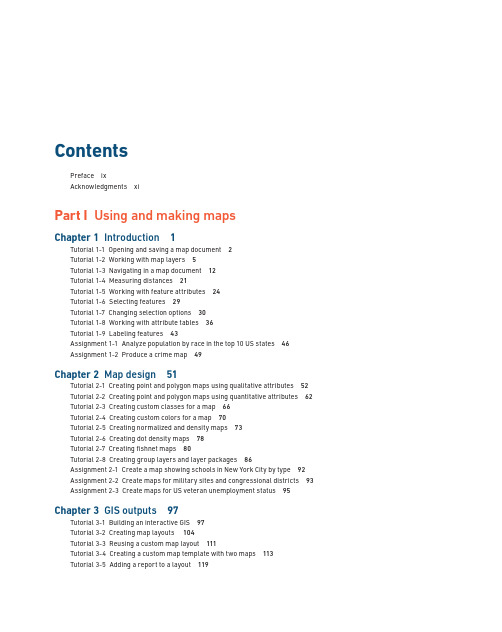
ContentsPreface ixAcknowledgments xiPart I Using and making mapsChapter 1 Introduction 1Tutorial 1-1 Opening and saving a map document 2Tutorial 1-2 Working with map layers 5Tutorial 1-3 Navigating in a map document 12Tutorial 1-4 Measuring distances 21Tutorial 1-5 Working with feature attributes 24Tutorial 1-6 Selecting features 29Tutorial 1-7 Changing selection options 30Tutorial 1-8 Working with attribute tables 36Tutorial 1-9 Labeling features 43Assignment 1-1 Analyze population by race in the top 10 US states 46Assignment 1-2 Produce a crime map 49Chapter 2 Map design 51Tutorial 2-1 Creating point and polygon maps using qualitative attributes 52 Tutorial 2-2 Creating point and polygon maps using quantitative attributes 62 Tutorial 2-3 Creating custom classes for a map 66Tutorial 2-4 Creating custom colors for a map 70Tutorial 2-5 Creating normalized and density maps 73Tutorial 2-6 Creating dot density maps 78Tutorial 2-7 Creating fishnet maps 80Tutorial 2-8 Creating group layers and layer packages 86Assignment 2-1 Create a map showing schools in New York City by type 92 Assignment 2-2 Create maps for military sites and congressional districts 93 Assignment 2-3 Create maps for US veteran unemployment status 95Chapter 3 GIS outputs 97Tutorial 3-1 Building an interactive GIS 97Tutorial 3-2 Creating map layouts 104Tutorial 3-3 Reusing a custom map layout 111Tutorial 3-4 Creating a custom map template with two maps 113Tutorial 3-5 Adding a report to a layout 119viGIS TUTORIAL FOR ARCGIS DESKTOP 10.8Tutorial 3-6 Adding a graph to a layout 121Tutorial 3-7 Building a map animation 123Tutorial 3-8 Using ArcGIS Online 128Assignment 3-1 Create a dynamic map of historic buildings in downtown Pittsburgh 128Assignment 3-2 Create a layout comparing 2010 elderly and youth population compositions in Orange County, California 130Assignment 3-3 Create an animation for an auto theft crime time series 131Part II Working with spatial dataChapter 4 File geodatabases 133Tutorial 4-1 Building a file geodatabase 133Tutorial 4-2 Using ArcCatalog utilities 136Tutorial 4-3 Modifying an attribute table 139Tutorial 4-4 Joining tables 142Tutorial 4-5 Creating centroid coordinates in a table 144Tutorial 4-6 Aggregating data 148Assignment 4-1 Investigate educational attainment 153Assignment 4-2 Compare serious crime with poverty in Pittsburgh 155Chapter 5 Spatial data 159Tutorial 5-1 Examining metadata 160Tutorial 5-2 Working with world map projections 162Tutorial 5-3 Working with US map projections 165Tutorial 5-4 Working with rectangular coordinate systems 167Tutorial 5-5 Learning about vector data formats 172Tutorial 5-6 Exploring raster basemaps from Esri web services 178Tutorial 5-7 Downloading raster maps from the USGS 181Chapter 6 Geoprocessing 185Tutorial 6-1 Extracting features for a study area 185Tutorial 6-2 Clipping features 190Tutorial 6-3 Dissolving features 192Tutorial 6-4 Merging features 195Tutorial 6-5 Intersecting layers 199Tutorial 6-6 Unioning layers 202Tutorial 6-7 Automating geoprocessing using ModelBuilder 208Assignment 6-1 Build a study region for Colorado counties 220Assignment 6-2 Dissolve property parcels to create a zoning map 222Assignment 6-3 Build a model to create a fishnet map layer for a study area 223Chapter 7 Digitizing 227Tutorial 7-1 Digitizing polygon features 228Tutorial 7-2 Digitizing line features 239Tutorial 7-3 Digitizing point features 245Tutorial 7-4 Using advanced editing tools 248Tutorial 7-5 Spatially adjusting features 255Assignment 7-1 Digitize police beats 259COnTEnTS viiAssignment 7-2 Use GIS to track campus information 261Chapter 8 Geocoding 263Tutorial 8-1 Geocoding data by ZIP Code 263Tutorial 8-2 Geocoding data by street address 268Tutorial 8-3 Correcting source addresses using interactive rematch 274Tutorial 8-4 Correcting street reference layer addresses 276Tutorial 8-5 Using an alias table 281Assignment 8-1 Geocode household hazardous waste participants to ZIP Codes 282Assignment 8-2 Geocode immigrant-run businesses to Pittsburgh streets 284Assignment 8-3 Examine match option parameters for geocoding 285Part III Analyzing spatial dataChapter 9 Spatial analysis 289Tutorial 9-1 Buffering points for proximity analysis 290Tutorial 9-2 Conducting a site suitability analysis 295Tutorial 9-3 Using multiple ring buffers for calibrating a gravity model 299Assignment 9-1 Analyze population in California cities at risk for earthquakes 308Assignment 9-2 Analyze visits to the Jack Stack public pool in Pittsburgh 310Chapter 10 ArcGIS 3D Analyst for Desktop 313Tutorial 10-1 Creating a 3D scene 314Tutorial 10-2 Creating a TIN from contours 315Tutorial 10-3 Draping features onto a TIN 320Tutorial 10-4 Navigating scenes 326Tutorial 10-5 Creating an animation 330Tutorial 10-6 Using 3D effects 332Tutorial 10-7 Using 3D symbols 335Tutorial 10-8 Editing 3D objects 339Tutorial 10-9 Using 3D Analyst for landform analysis 342Tutorial 10-10 Exploring ArcGlobe 348Assignment 10-1 Develop a 3D presentation for downtown historic sites 352Assignment 10-2 Topographic site analysis 354Assignment 10-3 3D animation of a conservatory study area 355Chapter 11 ArcGIS Spatial Analyst for Desktop 357Tutorial 11-1 Processing raster map layers 358Tutorial 11-2 Creating a hillshade raster layer 363Tutorial 11-3 Making a kernel density map 365Tutorial 11-4 Extracting raster value points 371Tutorial 11-5 Conducting a raster-based site suitability study 374Assignment 11-1 Create a mask and hillshade for suburbs 381Assignment 11-2 Estimate heart attack fatalities outside hospitals by gender 383Chapter 12 ArcGIS Network Analyst for Desktop 385Tutorial 12-1 Solving the “traveling salesperson” problem 386Tutorial 12-2 Building a TIGER-based network dataset 394viiiGIS TUTORIAL FOR ARCGIS DESKTOP 10.8Tutorial 12-3 Creating travel polygons 402Tutorial 12-4 Locating facilities 409Tutorial 12-5 Routing vehicles from depots to demand points 414Assignment 12-1 Geographic access to federally qualified health centers 421Assignment 12-2 Analyze visits to the Phillips public pool in Pittsburgh 423Assignment 12-3 Locate new farmers’ markets in Washington, DC 424Appendix Data source credits 427。

1、下载文档前请自行甄别文档内容的完整性，平台不提供额外的编辑、内容补充、找答案等附加服务。
2、"仅部分预览"的文档,不可在线预览部分如存在完整性等问题,可反馈申请退款(可完整预览的文档不适用该条件!)。
3、如文档侵犯您的权益，请联系客服反馈,我们会尽快为您处理(人工客服工作时间：9:00-18:30)。