Temperature gradients in XMM-Newton observed REFLEX-DXL galaxy clusters at z~0.3
多层介质传热的计算模拟

摘
*
要
在稳定热源流过多层介质材料的传热过程中,温度会随时间和位置发生变化。本文分析了稳定热源通过
通讯作者。
文章引用: 甄嘉鹏, 郭琦, 周江. 多层介质传热的计算模拟[J]. 应用物理, 2019, 9(1): 7-12. DOI: 10.12677/app.2019.91002
甄嘉鹏 等
多层介质传热的温度分布,运用热传导方程导出了热稳定后的温度分布以及最内层材料温度随时间的变 化关系。本文的方法适用于多种隔热材料的复合问题,可求出多层介质各层温度随时间的变化规律。
Keywords
Multi-Layered Media, Heat Transfer, Thermal Insulation Material
多层介质传热的计算模拟
甄嘉鹏1,郭
1 2
琦2,周
江1*
贵州大学物理学院,贵州 贵阳 贵州大学数学与统计学院,贵州 贵阳
收稿日期:2018年12月21日;录用日期:2019年1月4日;发布日期:2019年1月11日
由傅里叶定律和能量守恒定律得出温度随时间和位置变化的方程[8]:
Open Access
1. 引言
多层材料在传热过程中,不同介质材料会导致不同的温度分布。温度在材料内部随着位置而变化, 材料最内侧的温度会随热传递的时间而变化。 这类问题从 20 世纪 80 年代开始一直被广泛研究。 1981 年, 顾延安研究了保温层外壁面温度,以及它的计算方法,通过理论推导给出了一种计算热损失的方法[1]。 2007 年,白净选用第一类边界条件下的柱坐标形式的导热微分方程对圆筒壁内的温度分布进行计算和分 析,得出结论等温面的热流密度相同[2]。曾剑等考虑了一类热传导方程中间断扩散系数的反问题,证明 了时间相对较小时,极小元的唯一性和稳定性[3] [4] [5] [6]。2018 年,陈大伟利用热传导方程的差分格式 对一维热传导方程的数值解进行计算并绘成图, 从而直观地得到热传导媒介上的温度时空分布[7]。 目前, 对于热传导方程解的研究并以此得到热传导媒介在传热过程中的温度分布的相关研究仍在继续,然而对 于将两者与隔热材料相结合以提高复合材料的隔热性能以及对隔热时间的研究仍然较少。该研究对于复 合材料隔热性能的提高和隔热材料的选择具备参考价值,在实际生活中的应用也较为广泛,可应用于高 温作业服、消防隔热墙等诸多领域,因此具有一定的研究价值。 本文通过实验所得实验数据,利用数学物理方程建立稳定状态下的温度分布模型,包括复合介质各 分界面的温度变化和多层材料内侧温度随时间的变化。将该热传导模型和实验曲线进行对比,验证模型 的正确性。
功能梯度材料热传导问题的仿真

滑 连续地变 化。F M 因其 良好 的热力学 性能被 广泛应 用于 G
航 空航 天 、 核能 、 械等 领域 … 。由于功能 梯度 材料 大多在 机 高温环境下 工作 , 故对其进行热传导分 析以 了解其 温度分布
3 c ol f tr sSineadE gne n C ag nU iesy X’ hn i 104, hn ) .S ho o e a cec n n er g, h n’ nvrt, inS ax 70 6 C i Ma i l i i a i a a
ABS RACT : h u d me t ou in o se d T T e f n a n a s l t s t t a y—sae h a o d cin p o lm rt re tp sf n t n l r d d l o t t e tc n u t r be f e y e u c i a y g a e o o h ol
C O L i li, E in—zo g , HA G X e—m n , I i g A e—e P I a J hn Z N u i LU Qo n
( .Ke a oaoyfrR a o srcinT c n lg 1 yL b rtr o d C ntu t e h oo y& Eq ime t h n ’nUnv ri ,Xi n S ax 0 4,C ia; o o up n ,C a ga iest y ’ hn i 1 6 a 70 hn
1 ( ) 2r ) ( ) 7 ( “
(2 1)
因此 , 于指数型 F M, 对 G 其热传导方程 的基本解为
数值分析_Newton 迭代法画出最美的图形

r=-2:0.01:2
1 x4
13. m=1 a=1 d=4 tol=1e-5 maxIter=4 函数表达式: f ( x) 1 图示 pic013:
r=-2:0.01:2
1 x4
14. m=1 a=10 d=10 tol=1e-5 maxIter=5 函数表达式: f ( x) 1 图示 pic014:
r=-2:0.01:2
1 x10
5.
m=1 a=1 d=10 tol=1e-5 maxIter=5 函数表达式: f ( x) 1 图示 pic005:
r=-2:0.01:2
1 x10
6.
m=10 tol=1e-5
a=1 d=10 maxIter=10
r=-2:0.01:2
函数表达式: f ( x) 10 图示 pic006:
1 x10
7.
m=1000 tol=1e-5
a=1 d=10 maxIter=10
r=-2:0.01:2
函数表达式: f ( x) 1000 图示 pic007:
1 x10
8.
m=1 a=10 d=10 tol=1e-5 maxIter=10 函数表达式: f ( x) 1 图示 pic008:
r=-2:0.01:2
10 x10
15. m=1 a=10 d=10 tol=1e-10 maxIter=5 函数表达式: f ( x) 1 图示 pic015:
r=-2:0.01:2
10 x10
五、总结
1. 2. 3. 4. 函数 f(x)的变量的幂决定花瓣的数量,幂次越高花瓣数量越多,同时对花瓣的大小有一 定的影响。 迭代次数的多少影响花瓣与中心点的距离,迭代次数越多,花瓣离中心点越近,迭代次 数越少离中心点越远。 m 和 a 影响图形的放大效果,其中 m 越大,图形越小,而 a 越大图形越大,若 a/m 为 常数时,图形无变化。 误差 tol 衡量花瓣与中心点的距离,tol 越大,花瓣离中心点越近,越小越远。
thermal duct model derived by fin-theory approach and applied on an unglazed solar collector

A steady state thermal duct model derived by fin-theory approachand applied on an unglazed solar collectorB.Stojanovic´*,D.Hallberg,J.Akander Building Materials Technology,KTH Research School,Centre for Built Environment,University of Ga ¨vle,SE-80176Ga ¨vle,SwedenReceived 12November 2008;received in revised form 28January 2010;accepted 15June 2010Available online 24August 2010Communicated by:Associate Editor Brian NortonAbstractThis paper presents the thermal modelling of an unglazed solar collector (USC)flat panel,with the aim of producing a detailed yet swift thermal steady-state model.The model is analytical,one-dimensional (1D)and derived by a fin-theory approach.It represents the thermal performance of an arbitrary duct with applied boundary conditions equal to those of a flat panel collector.The derived model is meant to be used for efficient optimisation and design of USC flat panels (or similar applications),as well as detailed thermal analysis of temperature fields and heat transfer distributions/variations at steady-state conditions;without requiring a large amount of computa-tional power and time.Detailed surface temperatures are necessary features for durability studies of the surface coating,hence the effect of coating degradation on USC and system performance.The model accuracy and proficiency has been benchmarked against a detailed three-dimensional Finite Difference Model (3D FDM)and two simpler 1D analytical models.Results from the benchmarking test show that the fin-theory model has excellent capabilities of calculating energy performances and fluid temperature profiles,as well as detailed material temperature fields and heat transfer distributions/variations (at steady-state conditions),while still being suitable for component analysis in junction to system simulations as the model is analytical.The accuracy of the model is high in comparison to the 3D FDM (the prime benchmark),as long as the fin-theory assumption prevails (no ‘or negligible’temperature gradient in the fin perpendicularly to the fin length).Comparison with the other models also shows that when the USC duct material has a high thermal conductivity,the cross-sectional material temperature adopts an isothermal state (for the assessed USC duct geometry),which makes the 1D isothermal model valid.When the USC duct material has a low thermal conductivity,the heat transfer course of events adopts a 1D heat flow that reassembles the conditions of the 1D simple model (for the assessed USC duct geometry);1D heat flow through the top and bottom fins/sheets as the duct wall reassembles a state of adiabatic condition.Ó2010Elsevier Ltd.All rights reserved.Keywords:Unglazed solar collector;Roof integrated;Duct;Modelling;Fin-theory;Benchmarking1.IntroductionHeat transfer simulations and calculations on absorption of heat in flat-plate solar collectors,have generally been based on simplified one-dimensional (1D)heat transfer modelling (e.g.see:Duffie and Beckman,2006;Fischer et al.,2004).Traditionally,a fluid element flowing through the collector (or arbitrary duct)is assumed to absorb heatfrom its ambient in a 1D manner,along its flow path(Duffie and Beckman,2006).This approach renders a model that requires small computational resources and time,which is beneficial in system simulations when sea-sonal or annual performances are analysed.The efficiency and accuracy of the model is adequate for analysing energy performance,calculating bulk or outlet fluid temperatures,or ordinary absorber plate and fluid temperature distribu-tions (Duffie and Beckman,2006).If detailed analysis of temperature fields and heat transfer distributions/variations at steady-state or dynamic conditions are required,more0038-092X/$-see front matter Ó2010Elsevier Ltd.All rights reserved.doi:10.1016/j.solener.2010.06.016*Corresponding author.Tel.:+4626648137;fax:+4626648181.E-mail address:bojan.stojanovic@hig.se (B.Stojanovic´)./locate/solenerSolar Energy 84(2010)1838–1851sophisticated and complex models have to be used.For instance,this is needed when solar collectors have a duct/ tubefluid volume circumference that is significantly larger ()2)than the heat-absorbing surface.In this case regarding the duct/tube as a point in the absorber plate(e.g.Duffie and Beckman,2006;Hilmer et al.,1999)is not appropriate. Or in other cases,the thermal bridging between the absorb-ing surface and the backside,via the duct walls,cannot be neglected(Ammari,2003;Cristofari et al.,2002),nor the heat exchange between a duct wall and the collectorfluid (Ammari,2003;Hachemi,1999;Yeh et al.,2002).Detailed thermal modelling(of e.g.solar collectors)usually result in a multi-dimensional numerical model(e.g.Hassan and Bel-iveau,2007).The model can vary in complexity,depending on the desired level of detail.However,a detailed numerical model requires a substantial amount of computational power and time,which primarily makes it suitable and use-ful for specific and detailed case studies;not suitable as a component in system simulations.Furthermore,multi-dimensional numerical models have afixed geometrical lay-out of nodes/elements/volumes(depending on mathemati-cal discretisation principle),which makes the task of changing and comparing different solar collector designs tedious.In some cases there is a need to have a model which can calculate/simulate detailed thermal distributions and varia-tions,without requiring a large amount of pre-processing or computational power and time;thereby attaining a model suitable for component analysis while being useful in system simulations.The advantages are that solar collec-tor analysis and optimisation can be performed in junction to system operation at different geographical locations, during long-term simulation scenarios.As an example,this procedure is useful in durability assessments of solar collector absorber surfaces(e.g.see Carlsson et al.,1994).Annual simulations of solarNomenclatureA area(m2)bfin thickness(m)C equation constant(unit)C[T f(z)]equation constant as a function offluid temper-ature(unit)c heat capacity(J/K)c p specific heat capacity(J/kg K)d diameter(m)G global solar irradiance on a surface(W/m2)h heat transfer coefficient(W/m2K)K parameter for simplifying thefin temperature equation constants(–)Lfin length(m)q[x i,T f(z)]heatflux in an infinite smallfin element as a function of position in afin andfluid tempera-ture(W/m2)Q heat transfer rate(W)Q[x i,T f(z)]heat transfer rate in an infinite smallfin ele-ment as a function of(W)position in afin andfluid temperatureQ[T f(z)]heat transfer rate as a function offluid temper-ature(W/m)R thermal resistance(m2K/W)t time(s)T temperature(K)T(z)temperature as a function of USC duct length position(K)T(in)inlet temperature(K)T[x i,T f(z)]temperature as a function of position in afin andfluid temperature(K)V ambient air speed(m/s)U total heat loss coefficient(W/m2K)x coordinate parameter(–)y coordinate parameter(–)z coordinate parameter(–)_m massflow(kg/s)Nu Nusselt number(–)Greek symbolsa solar thermal absorptance(–)b parameter for simplifying thefin temperatureequation constants(unit)c[T f(z)]parameter as a function offluid temperature for simplifying thefin temperature equation con-stants(unit)D difference(–)e long wave(IR)emittance(–)j thermal conductance(W/K)k thermal conductivity(W/m K)q density(kg/m3)r Stefan–Boltzmann constant(W/m2K4) Subscriptsa ambientb backsideffluidh hydraulici nodal numberj nodal numberk nodal numberm materialn number of time-stepr radiations surfacefinfinsky skyUSC unglazed solar collectorB.Stojanovic´et al./Solar Energy84(2010)1838–18511839collectors operating in system solutions are performed atdifferent geographical locations,in order to assess the absorber surface microclimatic exposure to relevant degra-dation agents,such as temperatureet al.,1994;Van der Linden et al.,In general,durability issues of to a number of problems:lation or freezing (Wennerholm,issues are the exposure to various temperature,wind,rain/humidity,lutants)as a result of outdoor These contribute to a degradation tion of the collector material performance due to change in Carlsson et al.,1994;Stojanovic´assess this degradation,the tude of degradation agents (e.g.has to be detailed.Degradation nying degradation mechanisms and be strongly affected by for actively heated and cooled only be physicochemical activation values are passed.If only being degradation agents and assessment on degradation will in –time of wetness (TOW)is an degradation experiments exposure testing,e.g.see Carlsson that degradation agents and and that dose levels under a certain ute to a negligible rate of threshold values are exceeded.These changes in optical posed throughout the system,ciency (Hollands et al.,1992),economical and environmental a result of these types of changes,assessment is needed,so that the the performance lowering assessed.Work on assessing the mance due to solar collector tion of microclimate in/on solar of the most important steps (Carlsson et al.,1994;Hollands 2009).1.1.Background:a roof-integrated An unglazed solar collector the EU project Endothermic cient Housing in the EU unched in strated the use of a solar-assisted 2008;Stojanovic´,2009; e.g.see 2007)to provide the annual heating,cooling and hot water houses in different regions of the USC is a dual-purpose component that integrates with the building to form its roof (Virk,2008).The collector propi-tiously blends into its surroundings (different shapes and col-1840 B.Stojanovic´et al./Solar Energy 84(2010)1838–1851prevailing local climatic conditions.These modificationsconsisted in a variation of system:build-up,operation and control strategy.Regarding the USCs,no changes in the design of the component was made for the different systems,except for:coating colour,length of the extruded USC and number of USC panels used in the assembled system and rate of flow of the heat transfer fluid.The USC consists of an extruded aluminium profile which comes in two shapes,flat and bold rolled (see Fig.1).After extrusion,the ends are sealed and in-/outlet pipes are attached by welding.Thereafter,the panels are painted with a polyester powder coating.Each panel has a fixed:width (0.22m),number of ducts and material thickness (see also Table 2),while the length can vary up to a maximum of 6m.Feet and folds enable fixation onto the roof and inter-locking between adjacent panels.The following panel is interlocked to the previous and thereafter fixated.This forms an assembling chain that integrates the USCs into the roof and forms a homogenous surface.The heat transfer liquid flows through the panel in one homogenous direction,where each duct makes up an individual parallel flow streak (see Fig.2).The USC circuit has a flow regime that can vary from serial to parallel,depending on how the panels are con-nected.The fluid is distributed to and from the panels by a manifold.The fluid flow in the USC roof circuit is obtained via one or several circulation pumps.1.2.ObjectivesThis paper presents thermal modelling of the Endohous-ing USC flat panel that uses heat transfer liquids.The aimis to produce a detailed yet swift thermal steady-state model.The model is analytical,1D and derived by fin-the-ory approach.It represents the thermal performance of an arbitrary duct with applied boundary conditions equal to the flat panel USC;hence the model is also applicable for other thermal duct calculations.As the USC predomi-nantly consists of angular ducts,the traditional thermal modelling approach of the duct/tube being a point in the absorber is not appropriate (if detail analysis of tempera-ture fields and heat transfer distributions/variations is required);in this case the ducts constitute the absorber,hence the USC flat panel model development.The derived model is to be used for efficient optimisation and design of the USC flat panels (or similar applications),as well as detailed thermal analysis at steady-state conditions;with-out requiring a large amount of computational power and time.Detailed surface temperatures are necessary fea-tures of the fin-theory based USC thermal duct model in order to be useful for durability studies of the surface coat-ing,hence the effect of coating degradation on USC andsystem performance (see Section 1and reference Stojanovic´et al.,2008).The model accuracy and proficiency is bench-marked against a detailed 3D numerical model as well as two 1D analytical models.The paper objective is also to present results,discussion and conclusions of the different benchmarking models comparison,as these are commonly used for this type of application;in line with the work pre-sented by Schnieders (1997).1.3.Model assumptionsThis section represents a summary of assumptions applied in the derivation of the various USC thermal mod-els.Table 1displays which assumption is applicable to each model.1.The fluid temperature in each duct is equal,as the flow in the USC panel is parallel (see Section 1.1).The USC roof installation should also be seen as having a parallel circuit,as is the case in theSwedish Endosite system (Virk,2008;Stojanovic´,2009).2.The thermal effects of the feet and folds on the USC flat panel are neglected (see Figs.1and 3).Panel feet affect the USC by thermally bridging the duct assem-bly (especially the adjacent ducts)to the substrate by conduction.A roof integrated USC installation con-sists of a number of panels that are interlocked with each other,the last duct in one panel and the firstTable 2The geometrical dimensions of the modelled USC half duct;representing the actual dimensions of the flat panel USC developed and used in the Endohousing project.Note that the wall fin/sheet thickness is not eligible for the 1D simple steady-state C models Half duct inner with (m)Half duct inner height (m)Top and bottomfin/sheet thickness (m)Wall fin/sheet thickness (m)USC duct length (m)For all models0.01250.0130.0020.0015Table 1A summary of assumptions applied in the derivation of the various USC models.Assumption Fin-theory steady state 3D steady state FDM 1D isothermal steady state 1D simple steady state 1x x x x 2x x x x 3x x x x 4x x x x 5x x x x 6x x x 7x x x x 8x xx x 9xx x 10x11xNote :A detailed thermal analysis at the specific USC flat panel boundary conditions of the panel feet and the end duct wall is beyond the scope of this paper or the presented thermal duct models.B.Stojanovic ´et al./Solar Energy 84(2010)1838–18511841in a neighbouring panel will have a different build-up than a centrally placed duct.This is especially appar-ent at the duct wall,which will have a different heat transfer than the wall of a centrally placed duct.3.Boundary effects at the perimeter of the roof are neglected due to marginal impact on overall USC roof performance.4.The duct fluid temperature is isothermal (no temper-ature gradient,fully mixed)in each cross-section,except at the thermal boundary layer which gives rise to the convective heat transfer coefficient (Holman,2002).5.The average Nusselt number for(cross-section aspect ratio 1/2)wall heat flux and fully applied for the duct convection (1978).6.A linearisation of the equation energy (heat)transfer rate by tion (Duffie and Beckman,2006the discussion in Section 2.1.7.No heat exchange by long wave within the duct since the heat (see Section 1.1).8.Material,fluid and heat transfer exception of long wave stants,independent of 9.The model assumes that there is pendicular to the USC duct 10.The USC duct consists of a material cross-section.11.The USC duct consists of a temperature difference over and and the lower USC duct wall sheet/fin is adiabatic.The sheets/fins have each a their respective fin,which is length.2.Fin-theory based USC thermal model derivation A 1D steady state thermal model based on fin-theory isderived in order to obtain a tool that swiftly calculates and assesses the USC’s performance:material temperature and heat transfer distribution/variation and fluid temperature.This section presents the model derivation procedure.The basic concept of the 1D steady state fin-theory is that heat is transported from the fin-base throughout the fin-material in length direction;there is no ‘or negligible’temperature gradient in the fin perpendicularly to the fin length.While conduction prevails,heat is either emitted or absorbed by the fin depending on the interaction with the ambient (Holman,2002).The USC flat panel cross-section represented in Fig.3shows that a thermal symmetry can be applied on a USC flat panel duct,dividing it into a half duct.The USC half duct becomes a system of three fin sheets.Fig.4presents the thermal system with applied boundary conditions and defined energy flows used in the fin-theory based model.These boundary conditions represent the thermal course of event in a central duct on flat panel USC.As previously discussed,by adopting that statements 1,2and 3repre-sented in Section 1.3(see also Table 1),the heat transfer occurring in a centrally placed duct can be seen as repre-senting an entire USC panel or roof (see also Fig.3).Addi-tionally,please also observe the notification at the end of Section 1.3.Analytical thermal modelling of ducts in similar applica-tions has also been presented by Ammari (2003),Hachemi (1999)and Yeh et al.(2002).Ammari (2003)presents a Fig.3.A cross-section of the Endohousing flat panel USC.The figure shows the applied thermal symmetry lines on a centrally placed duct that makes a half duct,which is seen as representing the USC thermal behaviour.The models neglect the thermal effects of the two lower feet and the folds at each edge.Energy 84(2010)1838–1851air-heaters.In their models,the duct walls are seen as fac-tors that increase the thermal convection from duct sur-faces to the airflow.No thermal bridging by thermal conduction via the duct walls is applied.2.1.Mathematical derivationThe following example presents the derivation of the temperature distribution expression of Fin1(see Fig.5), which is the topfin/sheet of the USC half duct.The heat balance of over an infinite small element in a cross-section of Fin1is according to Figs.4and5as:Q1½x1;T fðzÞ þQ3½x1;T fðzÞ þQ4þQ5½x1;T fðzÞ¼Q6½x1;T fðzÞ þQ2½x1þdx1;T fðzÞ ð1ÞThe rate of heat conduction to the element at x1isQ1½x1;T fðzÞ ¼Àk1ÁA1ÁdT1½x1;T fðzÞdx1ð2Þand heat conduction from the element at position x1+dx1isQ2½x1þdx1;T fðzÞ ¼Àk1ÁA1ÁdT1½x1;T fðzÞdx1þddx1Àk1ÁA1ÁdT1½x1;T fðzÞdx1dx1ð3ÞHeat transfer rate by ambient(outdoor)convection:Q3½x1;T fðzÞ ¼h aÁA1:2ÁðT aÀT1½x1;T fðzÞ Þð4ÞThe outdoor wind convection coefficient h a used through-out this paper is according to Watmuffet al.(1977)as:h a¼2:8þ3:0ÁVð5ÞEnergy(heat)transfer rate by solar radiation:Q4¼aÁA1:2ÁG USCð6ÞEnergy(heat)transfer rate by long wave(IR)radiation (Duffie and Beckman,2006):ture T1[x1,T f(z)]is a function of bothfin length/position(x1) and USC ductfluid temperature along the duct length/posi-tion(z),a representative mean value of T1[x1,T f(z)]derived in an iterate manner is used in order to calculate h r.Heat transfer rate byfluid convection:Q6½x1;T fðzÞ ¼h fÁA1:2ÁðT1½x1;T fðzÞ ÀT fðzÞÞð8ÞThe ductfluid convection coefficient h f used throughout this paper is according to Holman(2002)as:h f¼NuÁk fd hð9Þwhere the average Nusselt number for a rectangular duct(cross-section aspect ratio1/2)with constant axial wall heatflux and fully developed laminarflow is Nu= 4.123(Shah and London,1978).The combination of the above-presented equations in accordance to Eq.(1)will give:d2T1½x1;T fðzÞdx1Àðh fþh aþh rÞk1Áb1|fflfflfflfflfflfflfflfflfflffl{zfflfflfflfflfflfflfflfflfflffl}b1ÁT1½x1;T fðzÞþh fÁT fðzÞþh aÁT aþaÁG USCþh rÁT skyk1Áb1|fflfflfflfflfflfflfflfflfflfflfflfflfflfflfflfflfflfflfflfflfflfflfflfflfflfflfflfflfflfflfflfflfflfflfflffl{zfflfflfflfflfflfflfflfflfflfflfflfflfflfflfflfflfflfflfflfflfflfflfflfflfflfflfflfflfflfflfflfflfflfflfflffl}c1½T fðzÞ¼0ð10ÞThe partial differential equation of the Fin1tempera-ture distribution becomes:d2T1½x1;T fðzÞdx1Àb1ÁT1½x1;T fðzÞ þc1½T fðzÞ ¼0ð11ÞThe solution to the partial differential equation in Eq.(11)is:T1½x1;T fðzÞ ¼C11½T fðzÞ ÁeÀffiffiffiffib1pÁx1þC12½T fðzÞ Áeffiffiffiffib1pÁx1þc1½T fðzÞb1ð12ÞThe procedure for deriving thefin-temperature distribu-tion for Fins2and3is in direct analogy with the above presented example.Fins2and3are applied with the boundary conditions and heat balances that are displayed in Fig.4and presented in Appendix A.In order to be able to calculate the cross-sectional tem-perature distribution in Fins1,2and3(Eqs.(12),(A3), and(A5)),the unknown constants in thefin-temperature equations have to be solved.By using boundary conditions as illustrated in Fig4and combining the heat transfer rates exiting from onefin and entering another,provides the pos-sibility to solve the unknown constants.Fin1dT1½x1¼0;T fðzÞ1¼0;Àk1ÁA1ÁdT1½x1¼L1;T fðzÞdx1¼Àk2ÁA2ÁdT2½x2¼0;T fðzÞdx2B.Stojanovic´et al./Solar Energy84(2010)1838–18511843Fin2T2½x2¼0;T fðzÞ ¼T1½x1¼L1;T fðzÞ T2½x2¼L2;T fðzÞ ¼T3½x3¼L3;T fðzÞFin3dT3½x3¼0;T fðzÞdx3¼0;Àk3ÁA3ÁdT3½x3¼L3;T fðzÞdx3¼k2ÁA2ÁdT2½x2¼L2;T fðzÞdx2The solved unknown constants of thefin-temperature distribution equation in a USC duct cross-section are defined and presented in Appendix A.By integrating the heatflux(containing thefin-tempera-ture distribution)over the entirefin length attains the heat transfer rate from afin cross-section.Eq.(13)presents the heat transfer rate from Fin1to the USCfluid(see also Fig.4).An example of the derivation of the heat transfer rate equations to and from the USC half duct is presented in Appendix A.Q6½T fðzÞ ¼Àh fÁÀC11½T fðzÞ Áb1þC12½T fðzÞ Áb1þC11½T fðzÞ ÁeðÀffiffiffiffib1pÁL1ÞÁb1ÀC12½T fðzÞ Áeðffiffiffiffib1pÁL1ÞÁb1Àc1½T fðzÞ ÁL1Áffiffiffiffiffib1pþT fðzÞÁL1Ábð3=2Þ1 0@1Ab1ð13ÞHaving derived heat transfer rates from thefin cross-sec-tions to the USCfluid,provides the possibility to calculate thefluid temperature along the USC duct,hence thefin-temperature distribution.Eq.(14)presents the steady state fluid temperature along the USC duct.The equation assumes that there is no heat transfer perpendicular to the USC duct cross-section.T fðzÞ¼T fðinÞþC2 C1Áe zÁC1_mÁc p fÀC2C1ð14ÞBy attainment of Eq.(14),thefin-temperature distribu-tion at a USC duct cross-section,as well as along the USC duct,can be calculated at steady-state conditions.The der-ivation of Eq.(14)and definition of equation constants are presented in Appendix A.3.Benchmarking modelsThe prime objective of the benchmarking models is to be used as a comparison for thefin-theory derived USC ther-mal duct model,in order to investigate calculated/simulated results deviations,but also as a comparison amongst themselves.3.1.1D isothermal steady-state modelThis model is based on the assumption that the thermal conductivity of the duct material is infinitely large,thus making the USC duct material cross-section isothermal. Other assumptions applied are listed in Table1;please also see the discussion in the beginning of Section2.The model is basically‘equivalent’to the Hottel–Whiller–Bliss model as presented by Duffie and Beckman(2006).As the USC duct(in this case)constitutes the absorber plate,there is no absorber plate surface that is without direct contact with the ductfluid.By applying this case to the Hottel–Whiller–Bliss model(as presented by Duffie and Beckman (2006))and neglecting the bond thermal resistance between the absorber plate and tube/duct,brings that the duct material(fin)temperature is isothermal;as the model regards the duct as a point in the absorber plate cross-sec-tion.Fig.6illustrates the model set-up.The heat balance of afluid element,having the massflow_m in z-direction and temperature T f(z),gives that the increase influid tempera-ture dT f(z)due to heat supply corresponds to:h fÁðL1þL2þL3ÞÁdzÁðT s½T fðzÞ ÀT fðzÞÞ|fflfflfflfflfflfflfflfflfflfflfflfflfflfflfflfflfflfflfflfflfflfflfflfflfflfflfflfflfflfflfflfflfflfflfflfflfflfflffl{zfflfflfflfflfflfflfflfflfflfflfflfflfflfflfflfflfflfflfflfflfflfflfflfflfflfflfflfflfflfflfflfflfflfflfflfflfflfflffl}Q6½T fðzÞ þQ9½T fðzÞ þQ12½T fðzÞ¼h aÁL1ÁdzÁðT aÀT s½T fðzÞ Þ|fflfflfflfflfflfflfflfflfflfflfflfflfflfflfflfflfflfflfflfflfflfflfflffl{zfflfflfflfflfflfflfflfflfflfflfflfflfflfflfflfflfflfflfflfflfflfflfflffl}Q3½T fðzÞþaÁG USCÁL1Ádz|fflfflfflfflfflfflfflfflfflfflfflffl{zfflfflfflfflfflfflfflfflfflfflfflffl}Q4þh rÁL1ÁdzÁðT skyÀT s½T fðzÞ Þ|fflfflfflfflfflfflfflfflfflfflfflfflfflfflfflfflfflfflfflfflfflfflfflfflffl{zfflfflfflfflfflfflfflfflfflfflfflfflfflfflfflfflfflfflfflfflfflfflfflfflffl}Q5½T fðzÞþU bÁL3ÁdzÁðT bÀT s½T fðzÞ Þ|fflfflfflfflfflfflfflfflfflfflfflfflfflfflfflfflfflfflfflfflfflfflfflfflffl{zfflfflfflfflfflfflfflfflfflfflfflfflfflfflfflfflfflfflfflfflfflfflfflfflffl}Q13½T fðzÞð15ÞThe equation above can be reformulated with constants C1,C2and C3as expressed below.C1¼aÁL1ÁG USGþh aÁL1ÁT aþh rÁL1ÁT skyþU bÁL3ÁT bh aÁL1þh rÁL1þU bÁL3þh fÁðL1þL2þL3Þð16ÞC2¼Àðh aÁL1þh rÁL1þU bÁL3Þðh aÁL1þh rÁL1þU bÁL3þh fÁðL1þL2þL3ÞÞð17ÞC3¼h fÁðL1þL2þL3Þ_mÁc pfð18ÞLocal cross-sectional material/surface isotherm can accordingly be found such that:T s½T fðzÞ ¼aÁG USCÁL1þh aÁL1ÁT aþh rÁL1ÁT skyþU bÁL3ÁT bþh fÁðL1þL2þL3ÞÁT fðzÞf123a1r1b3ð19ÞConsidering that the inlet temperature T f(in)will increase to be the outlet temperature T f(z)at the duct length z,the heat balance of thefluid element can be inte-grated such that:Z T fðzÞT fðinÞdT fðzÞC1þC2ÁT fðzÞ¼C3ÁZ zdzð20ÞThe solution for Eq.(20)isfinallyT fðzÞ¼T fðinÞþC1C2Áe C2ÁC3ÁzÀC1C2ð21Þ1844 B.Stojanovic´et al./Solar Energy84(2010)1838–1851。
双U型地埋管换热器换热性能模拟分析
第52卷第6期2021年6月中南大学学报(自然科学版)Journal of Central South University (Science and Technology)V ol.52No.6Jun.2021双U 型地埋管换热器换热性能模拟分析杨培志1,陈嘉鹏1,陈君文2,李明3(1.中南大学能源科学与工程学院,湖南长沙,410083;2.中航长沙设计研究院有限公司,湖南长沙,410014;3.湖南凌天科技有限公司,湖南湘潭,410005)摘要:针对垂直双U 型地埋管换热器,在MATLAB 平台上建立热渗耦合作用下地埋管换热器的三维数值传热模型,并通过岩土热响应试验验证该模型的正确性。
基于建立的三维数值传热模型,分析U 型管内水流速度、回填材料热物性参数、地下水渗流速度及地下水水位对地埋管换热器换热性能的影响。
研究结果表明:当U 型管内水流速度从0.1m/s 增大到0.2m/s 时,可以明显提高地埋管换热器的换热性能;与增大导热系数相比,增大容积比热对提升地埋管换热器换热性能不明显;当地下水渗流速度从0m/a 增大到35m/a 时,地埋管换热器与土壤的换热效果明显;地下水位对地埋管换热器换热性能有较大影响。
关键词:地埋管换热器;三维数值传热模型;地下水渗流;岩土热响应试验中图分类号:TK52文献标志码:A文章编号:1672-7207(2021)06-1733-06Simulation and analysis of heat transfer performance of doubleU-tube ground heat exchangersYANG Peizhi 1,CHEN Jiapeng 1,CHEN Junwen 2,LI Ming 3(1.School of Energy Science and Engineering,Central South University,Changsha 410083,China;2.China Aviation Changsha Design and Research Co.Ltd.,Changsha 410014,China;3.Hunan Linten Science and Technology Co.Ltd.,Xiangtan 410005,China)Abstract:A three-dimensional numerical model of double U-tube ground heat exchangers (GHEs)was presented with heat transfer and groundwater seepage in MATLAB platform,which was verified by rock-soil thermal response test.Based on the established three-dimensional numerical heat transfer model,the influence of flow rate of U-shaped tube,thermophysical properties of grout,seepage flow rate and groundwater level on heat exchange performance of GHEs was analyzed.The results show that when U-tube water flow rate is from 0.1m/s to 0.2m/s,DOI:10.11817/j.issn.1672-7207.2021.06.001收稿日期:2021−01−10;修回日期:2021−03−15基金项目(Foundation item):国家自然科学基金面上资助项目(51276226)(Project(51276226)supported by the National NaturalScience Foundation of China)通信作者:杨培志,博士,副教授,从事制冷与空调技术的开发及应用研究;E-mail:*******************.cn引用格式:杨培志,陈嘉鹏,陈君文,等.双U 型地埋管换热器换热性能模拟分析[J].中南大学学报(自然科学版),2021,52(6):1733−1738.Citation:YANG Peizhi,CHEN Jiapeng,CHEN Junwen,et al.Simulation and analysis of heat transfer performance of double U-tube ground heat exchangers[J].Journal of Central South University(Science and Technology),2021,52(6):1733−1738.第52卷中南大学学报(自然科学版)the heat transfer performance of the buried tube heat exchanger can significantly be improved.Increasing the volume specific heat to enhance the heat transfer performance of buried tube heat exchanger is not obvious compared to increasing the thermal conductivity.When groundwater percolation rate is from0m/a to35m/a,the buried tube heat exchanger with soil′s heat transfer effect is obvious.The depth of the groundwater level on the buried tube heat exchanger has greater impact on the heat transfer performance.Key words:ground heat exchangers;3D numerical model;groundwater seepage;rock-soil thermal response test随着全球能源与环境问题的日益突出,能源的高效利用与环保已经越来越受到人们的重视。
牛顿热度模型-概述说明以及解释

牛顿热度模型-概述说明以及解释1.引言文章1.1 概述部分的内容:概述:牛顿热度模型是一种常用的热度计算模型,它基于牛顿冷却定律的基本原理,用于衡量和评估一个事物或事件的热度程度。
热度模型的概念起源于传热学领域,后来被应用到社会科学和媒体研究等领域。
本文将详细介绍牛顿热度模型的定义、应用领域以及其优缺点,并对其进行总结和展望。
通过深入探讨牛顿热度模型,我们可以更好地理解和评估事物的热度,并为未来的研究和实践提供指导和建议。
文章结构:本文共分为三个部分:引言、正文和结论。
引言部分对牛顿热度模型进行了概述,并介绍了本文的结构和目的。
正文部分主要包括牛顿热度模型的定义、应用领域以及其优缺点的详细讨论和解析。
结论部分对牛顿热度模型进行了总结,并展望了其未来的发展方向。
同时,结论部分也提出了一些相关的建议。
目的:本文旨在全面介绍和解析牛顿热度模型,并探讨其在各个领域的应用。
通过阐述牛顿热度模型的定义、优缺点以及未来发展的展望,我们希望读者能够更好地理解和应用该模型,为相关领域的研究和实践提供借鉴和指导。
同时,本文也将对牛顿热度模型进行全面评估和分析,以期为未来的发展和创新提供一定的参考和建议。
文章的编写将会着重围绕以上内容展开,通过对牛顿热度模型的阐述和分析,我们将全面展示其在实际应用中的价值和意义。
同时,通过对优缺点的讨论和总结,我们可以进一步改进和完善该模型,提高其应用的准确性和可靠性。
最后,我们将对牛顿热度模型的未来发展进行展望,并提出一些相关的建议,以期为相关研究和实践提供一定的指导和启示。
1.2文章结构文章结构部分的内容可以从以下几个方面来描述:1. 文章的布局和章节划分:说明文章的整体结构和章节划分,以帮助读者更好地理解文章的内容和组织。
例如,可以介绍文章由引言、正文和结论三个部分组成,每个部分又包含若干小节。
2. 引言部分的目的和内容:简要介绍引言部分的目的和内容,说明引言的作用是为了引起读者的兴趣、提出问题或背景、阐述研究背景等。
newton冷却问题数学建模python
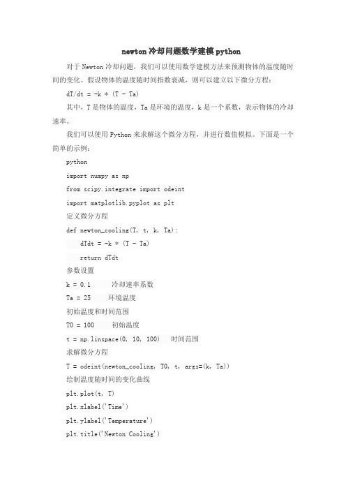
newton冷却问题数学建模python对于Newton冷却问题,我们可以使用数学建模方法来预测物体的温度随时间的变化。
假设物体的温度随时间指数衰减,则可以建立以下微分方程:dT/dt = -k * (T - Ta)其中,T是物体的温度,Ta是环境的温度,k是一个系数,表示物体的冷却速率。
我们可以使用Python来求解这个微分方程,并进行数值模拟。
下面是一个简单的示例:pythonimport numpy as npfrom scipy.integrate import odeintimport matplotlib.pyplot as plt定义微分方程def newton_cooling(T, t, k, Ta):dTdt = -k * (T - Ta)return dTdt参数设置k = 0.1 冷却速率系数Ta = 25 环境温度初始温度和时间范围T0 = 100 初始温度t = np.linspace(0, 10, 100) 时间范围求解微分方程T = odeint(newton_cooling, T0, t, args=(k, Ta))绘制温度随时间的变化曲线plt.plot(t, T)plt.xlabel('Time')plt.ylabel('Temperature')plt.title('Newton Cooling')plt.show()在以上代码中,我们使用了NumPy库来创建时间范围t,使用SciPy库中的odeint函数来求解微分方程。
最后使用Matplotlib库绘制温度随时间的变化曲线。
您可以根据实际情况调整参数和时间范围,以获得不同条件下物体温度的变化曲线。
华科能源学院版传热学

2013-8-4
5
华中科技大学热科学与工程实验室
HUST Lab of Thermal Science & Engineering
t1
t1
t1
t1
t0 A B C D A B C D
t0 A B C D
t0 A B C DFra bibliotekt0(a) = 1
tA tB tC tD
3
(b) = 2
(c) = 3
(b) (a) t∞ (c)
t
x
0
x
2013-8-4
11
华中科技大学热科学与工程实验室
HUST Lab of Thermal Science & Engineering
曲线(c)表示平板外环境 的换热热阻 1 h 远大于平 板内的导热热阻 , 即 1/ h / 从曲线上看,物体内部的温 度几乎是均匀的,这也就说 物体的温度场仅仅是时间的 函数,而与空间坐标无关。 我们称这样的非稳态导热系 统为集总参数系统(一个等 温系统或物体)。
2013-8-4
20
华中科技大学热科学与工程实验室
HUST Lab of Thermal Science & Engineering
hA hV A2 h(V / A) a BiV FoV 2 2 cV A cV (V / A)
l 物体内部导热热阻 Bi = 1 h 物体表面对流换热热阻 hl
2013-8-4
(b) (a) t∞
t
(c)
x
0
x
10
华中科技大学热科学与工程实验室
HUST Lab of Thermal Science & Engineering
- 1、下载文档前请自行甄别文档内容的完整性,平台不提供额外的编辑、内容补充、找答案等附加服务。
- 2、"仅部分预览"的文档,不可在线预览部分如存在完整性等问题,可反馈申请退款(可完整预览的文档不适用该条件!)。
- 3、如文档侵犯您的权益,请联系客服反馈,我们会尽快为您处理(人工客服工作时间:9:00-18:30)。
a r X i v :a s t r o -p h /0306115v 4 22 S e p 2003Astronomy &Astrophysics manuscript no.ms February 2,2008(DOI:will be inserted by hand later)Temperature gradients in XMM-Newton observed REFLEX-DXLgalaxy clusters at z ∼0.3⋆Y.-Y.Zhang 1,A.Finoguenov 1,H.B¨o hringer 1,Y.Ikebe 1,2,K.Matsushita 1,3,and P.Schuecker 11Max-Planck-Institut f¨u r extraterrestrische Physik,Giessenbachstraße,85748Garching,Germany2Joint Center for Astrophysics,University of Maryland,Baltimore Country,1000Hilltop Circle,Baltimore,MD 21250,USA3Tokyo University of Science,Tokyo,JapanReceived 5June 2003/accepted 22September 2003Abstract.We present XMM-Newton results on the temperature profiles of a volume-limited sample of galaxy clusters at redshifts z ∼0.3,selected from the REFLEX survey (REFLEX-DXL sample).In the spectral analysis,where only the energies above 1keV were considered,we obtained consistent results on the temperature derived from the pn,MOS1and eful temperature measurements could be performed out to radii with overdensity 500(r 500)for all nine clusters.We discovered a diversity in the temperature gradients at the outer cluster radii with examples of both flat and strongly decreasing profiing the total mass and the gas mass profiles for the cluster RXCJ0307.0−2840we demonstrate that the errors on the mass estimates for the REFLEX-DXL clusters are within 25%up to r 500.Key words.cosmology:observations –galaxies:clusters:general –X-rays:galaxies:clusters1.IntroductionThe number density of galaxy clusters probes the cosmic evolution of large-scale structure (LSS)and thus provides an effective test of cosmological models.It is sensitve to the matter density (Ωm )and the amplitude of the cosmic power spectra on cluster scale (σ8)(e.g.Schuecker et al.2003).Its evolution is sensitive to the dark energy (ΩΛ)(e.g.Vikhlinin et al.2002).The most massive clusters are especially important in tracing LSS evolution since they are expected to show the largest evolutionary effects.In addition,the X-ray properties of the most massive clus-ters should be easier to describe in hierarchical model-ing since the structure of the X-ray emitting intracluster plasma is essentially determined by gravitational effects and shock heating.With decreasing cluster mass and in-tracluster medium (ICM)temperature,non-gravitational effects play an important role before and after the shock heating (Voit &Bryan 2001;Voit et al.2002;Zhang &Wu 2003;Ponman et al.2003).Therefore,the most massive2Zhang et al.:Temperature gradients in XMM-Newton observed REFLEX-DXL galaxy clusters at z∼0.3pilation of some observational information on the nine REFLEX-DXL clusters.Col.(1):Cluster name. Cols.(2–3):Sky coordinates.Cols.(4–6):Net exposure time of MOS1,MOS2and pn after cleaning for theflaring episodes.Cols.(7–9):Light curve cleaning upper limit.Col.(10):Hydrogen column density in units of1020cm−2 (Dickey&Lockman1990).Col.(11):Revolution of XMM-Newton.Col.(12):Alternative nameClusterα(o)δ(o)Exposure Time(s)Criteria(cts/100s)n H orbit Alternative (RXCJ)Eq.J2000.0MOS1MOS2pn MOS1MOS2pn nameZhang et al.:Temperature gradients in XMM-Newton observed REFLEX-DXL galaxy clusters at z∼0.33 We use the XMMSAS v5.4software for data reduction.The MOS and pn data were taken in standard Full Framemode and Extended Full Frame mode,respectively.Forall detectors,the thinfilter has been used.Above10keV,there is little X-ray emission from theclusters due to the low telescope efficiency at these ener-gies;the particle background therefore completely domi-nates.The cluster emission is not variable,so any spec-tral range can be used for temporal variability studies ofthe background.Therefore,the10–15keV energy band(binned in100s intervals)was used to monitor the parti-cle background and to excise periods of high particleflux.In this screening process we use the settings F LAG=0and P AT T ERN<5for pn,and P AT T ERN<13forMOS.As an example,Fig.1shows the10–15keV pn lightcurve of RXCJ0658.5−5556.We reject those time intervals affected byflares inwhich the detector countrate(ctr)exceeds a thresholdof2σabove the average ctr,where the average and thevariance have been interactively determined from the ctrhistogram below the rejection threshold.A similar clean-ing criterion is applied to the screening of the backgroundobservation.We note,however,that the thresholds willbe different for the source and background accumulations.Formal freezing of the cleaning criterion does not overcomethe difference in the mean background ctr.In our analysiswe searched through a number of background observationstofind the one matching our target observations.The se-lection criterion is therefore tofind the one with a similarcleaning threshold.As shown in Table1,the pn and MOS detectors allhave their own similar cleaning thresholds for all obser-vations.In Sect.2.2we consider in detail how this back-ground behaviour affects the temperature determination.In the analysis of the pn data,we statistically removethe out-of-time effect by creating an out-of-time(OOT)Table2.Parameters of the residual background modelsfitted in the0.4–15keV band.Col.(1):Cluster name.Cols.(2–4):Index of the“powerlaw/b”residual back-ground model for MOS1,MOS2and pn.Cols.(5–7):Normalization at1keV of the“powerlaw/b”residualbackground model scaled to1arcmin2area for MOS1,MOS2and pn in units of10−4cts s−1keV−1arcmin−2.Cluster Index Normalization(RXCJ)MOS1MOS2pn MOS1MOS2pn4Zhang et al.:Temperature gradients in XMM-Newton observed REFLEX-DXL galaxy clusters at z∼0.3are rejected through the analysis of the light curve(e.g. Read&Ponman2003).However,we sometimes still ob-serve a residual enhancement of the background associ-ated with an increase in the quietflux of soft protons.The typical time-scale for the variation of this‘quiet’compo-nent is comparable to or exceeds the typical observational time-scale.Therefore,it is in general not possible to re-move observational intervals affected by this enhancement. Chen et al.(2003)describe an example of such an obser-vation where quite different‘quiet’background levels are observed before and after aflare,respectively.The photon background consists of foreground emis-sion from the Galaxy as well as the Cosmic X-ray Background(CXB).Observations of the blankfield also contain both components,provided the accumulations are done with the same instrumental set-up(e.g.with a par-ticularfilter)and the spectra of the X-ray background are the same for both the target and the blankfield.This is only guaranteed for the CXB and the emission from the Galaxy halo.Since the Galaxy also plays a role as absorber and foreground emitter,it is important to have a similar absorbing column density for both the target and back-ground accumulations.Additionally,there are some extra Galactic components,that display spatial variations.To constrain them,one has to look into the ROSAT All-Sky Survey data around both the background accumulations and the target.Observations with normal conditions of the Galactic emission are referred to the quiet Galactic zones.So are most of the X-ray background accumula-tions(Lumb et al.2002;Read&Ponman2003).Some source removal is performed on the existing background accumulations.This changes the shape and intensity of the residual CXB.Therefore,a similar source removal has to be performed in the analysis of the target.Several available XMM-Newton pointings have been investigated.We conclude that the XMM-Newton point-ings in the Chandra Deep Field South(CDFS)have sim-ilar background conditions as most targets and sufficient exposure time.Therefore,the CDFS is a good candidate for the background for our study.However,there is still a small difference between the background of our sources and the CDFS,e.g.the background ctr in the target ob-servations is slightly higher(10–20%)than in the CDFS, which we ascribe mostly to the contamination by soft pro-tons.We have carefully planned this cluster study such that the radii in which the cluster emission can be observed extent up to spherical overdensities of500,i.e.,the ratio of the mean density of the dark halo with respect to the redshift-dependent critical densityρcrit(z).This is the re-gion to which the cluster X-ray emission is expected to be essentially confined,covering about half of thefield of view (FOV)of the XMM-Newton telescope.This enables us to extract a source spectrum from the background region of the targetfield for comparison with a background spec-trum from the backgroundfield extracted with the same detector coordinates.Our residual background modeling procedure consists of analysing such regions not affected by cluster emission.We assume little or no vignetting of the soft proton induced background,as suggested by re-cent studies(Lumb et al.2002).Spectra are extracted from the9.2–11.5′region from the pointing center for our source observations and background candidate observa-tions.In afirst step,we compare the spectra extracted from the outer regions in the0.4–15keV band between the sources and the background pointings.The residual background signal found after the subtraction of the back-groundfield from the targetfield in this outer area is then modeled by a power law spectrum(model“powerlaw/b”in XSPEC,a power law background model which is con-volved with the instrumental redistribution matrix but not with the effective area).We use this model to account for the excess soft proton background in our observations as compared to the backgroundfield.This residual power law background model is introduced over the whole energy range(“wabs∗mekal+powerlaw/b”,an emission spectrum from hot diffuse gas,e.g.Mewe et al.1985,considering the Galactic absorption and modeling the residual back-ground by a power law),which yields the correct shape of the background component after the combination with the blankfield background(double background subtrac-tion method).During this procedure,the normalization of the residual background component is always scaled to the area of the source extraction region.In Fig.2we present examples of the residual back-ground.The parameters of the residual background mod-elsfitted in the0.4–15keV band for the clusters are given in Table2.The residual background in pn is higher than in MOS because the larger thickness of the pn-pixels leads to a higher sensitivity to the particleflux.Since the sub-traction of the residual background is only a second or-der correction to the data and because of the large noise in the residual background data,we are not attempting a perfect modelfitting,but approximating the data by a simple power law model.The uncertainty in the nor-malization is,anyway,within5%and10%for MOS and pn,respectively.The correction due to the residual back-ground makes only a1–4%effect in the cluster signals and an up to10%effect to the temperature determinations for cluster radii r≤4′.At larger radii the effect of the correct background effect is large as shown in Fig.3,but the un-certainty in the approximation of the residual background –a third order effect–is still small.To recover the correct spectral shape and normaliza-tion of the cluster component,we need both the response matrixfile(rmf)and auxiliary responsefile(arf).The following need to be taken into account in either rmf or arf:(i)Pure redistribution matrix giving the probability that a photon of energy E,once detected,will be measured in data channel PI.(ii) Quantum efficiency(with closedfilter position)of the CCD detector.(iii)Filter transmission.(iv) Geometric factors such as bad pixel corrections and gap corrections(around4%).(v)Telescope effective area as a function of photon energy.(vi) Vignetting correction to effective area for off-axisZhang et al.:Temperature gradients in XMM-Newton observed REFLEX-DXL galaxy clusters at z∼0.35 pointings.We choose the rmf which correspondsto(i)and(ii)(with closedfilter position).The pnrmf that corresponds to this choice has a‘6Zhang et al.:Temperature gradients in XMM-Newton observed REFLEX-DXL galaxy clusters at z∼0.3 The global temperatures obtained from modelfits tothe larger spectral range0.4–10keV are always lowercompared to the temperatures obtained from1–10keV.To check if the discrepancy is partially due to residualGalactic emission,we undertake the following test.Weextract the spectra from the inner(hereafter“A”)andouter(hereafter“B”)parts of the background region inboth the background(hereafter“bkg”)and target(here-after“src”)observations.If there is some difference inthe Galactic emission between the background and targetobservations,there must be some residual Galactic emis-sion after we subtract the spectrum“B(src)−B(bkg)”,scaled by the area of the region A,from the spectrum“A(src)−A(bkg)”because of the vignetting effect of theGalactic emission.We apply a thermal emission spectralmodel(“apec”)with all parameters free in XSPEC tofit this residual emission.We found that the temperatureof this component is around0.2keV and the redshift isclose to zero.In the following analysis,wefix the tempera-ture to0.2keV,the abundance to solar abundance and theredshift to zero,and obtain the normalization of this com-ponent.We re-analyse the global properties of the clustersintroducing the residual Galactic emission normalized bythe area and vignetting effect.Since the difference in thetemperatures determined in the0.4–10keV and1–10keVbands still remains,we report the temperature measure-ments setting the normalization of the residual Galacticemission to its upper limit(cf.Table4).However,thiscomponent only makes a<1%effect in the cluster sig-nals.It is thus clear that the discrepancy is not or notmainly due to the residual Galactic emission.This dis-crepancy will again be discussed below.Table3.Regions with substructures and point sourcesexcluded from the analysis.Col.(1):Cluster name.Col.(2–3):Center of the circle in sky coordinates for J2000.0.Col.(4):Radii.Col.(5):“Yes”if there is an optical point-like counterpart in a digitized optical survey(e.g.DSS2).Cluster(RXCJ)α(o)δ(o)r(′′)optZhang et al.:Temperature gradients in XMM-Newton observed REFLEX-DXL galaxy clusters at z∼0.37 0.4–12keV band.In this case a high temperature of k B T=18.8±2.1keV was obtained while the n H went down toan unrealistically small value of1.8±0.5×1020cm−2,al-though the remaining parameters were still relatively rea-sonable.Therefore,we decide tofix n H=6.5×1020cm−2,but exclude the soft band(0.4–2keV).In this case we ob-tained stable results for the temperature,metallicity,andredshift(see Table4).No significant metallicity gradientswere found in our analysis.We notice that the temperature of RXCJ0528.9−3927(also in other clusters)changes significantly with the lowcut-offof the energy band used in thefit.In Fig.7,we thus used the X-ray spectra to test the energy banddependence and possible method dependencies by com-paring the temperature measurements versus low energyband(low-E)cut-offfrom two different methods(the dou-ble background subtraction method and the method ap-plied in Arnaud et al.2002,i.e.we use the standardXMMSAS command‘evigweight’to correct vignetting,use‘arfgen’and‘rmfgen’to create on-axis arf and rmf,and apply the blank sky provided by Lumb2002).Forcomparison,we applied the following models tofit thespectra in the0.4–10keV band after double backgroundsubtraction.We obtain k B T=7.69+0.28−0.46keV and n H∼0−0.1×1020cm−2using a single-phase temperature model(“wabs∗mekal+powerlaw/b”)with free n H.We obtain k B T=10.12±3.13keV using two component thermal model(“wabs∗(mekal+powerlaw)+powerlaw/b”)withfixed n H.We also obtain k B T1=9.34+5.93−1.04keV andk B T2∼0.49−1.34keV using two thermal component model(“wabs∗(mekal+apec)+powerlaw/b”),in which we fix the redshift of the soft component to the redshift of the cluster.The metallicity and redshift measurements among the different modelings and different low-E cut-offvary within5%.The results presented in Fig.7suggest some influence of the low energy band on the temperature mea-surements.As we discussed above,the results obtained in the harder energy band should recover the correct cluster temperature.Similar phenomena are also found for A1413 (Pratt&Arnaud2002)using XMM-Newton data,and Coma,A1795and A3112(Nevalainen et al.2003)based on the comparison of XMM-Newton and ROSAT PSPC observations.Nevalainen et al.interprete this as a soft ex-cess,possibly due to a‘warm-hot’intergalactic medium. We will analyse this feature of our sample in more detail in a forthcoming paper.3.2.Temperature profilesWe have already noted that the differences between the global temperatures of the regions covering radii of0.5< r<4′and r<8′,respectively,in Table4are possi-bly caused by systematic temperature gradients.For a more detailed study of the temperature profiles we de-vide the cluster regions into thefive annuli0–0.5′,0.5–1′, 1–2′,2–4′,and4–8′(cf.Fig.3).Note that in the spectra extracted from the outermost rings of RXCJ0014.3−3022and RXCJ0528.9−3927we ignore a narrow energy band containing the residual background around the1.49keV Al line(Freyberg et al.2002).Table5shows the temperature profile catalogue of the clusters from the spectral analysisfitted by one or two step background subtraction(“mekal∗wabs”,“mekal∗wabs+powerlaw/b”).We use both the>0.4keV and>1keV energy bands except for RXCJ0658.5−5556. We apply the2–12keV band for this high temperature cluster.The temperature profiles of the clusters are also shown in Fig.6.For most of the objects,the temperature can be mea-sured out to r500.The overall temperature profile is char-acterized by a rather moderate decrease towards the cen-ter,and a decrease towards the outer regions,yet on dif-ferent levels,including no decrease at all for some of the clusters.This confirms a suggestion of Finoguenov et al. (2001b)that the differences in the behaviour of the tem-perature profiles in the outskirts of clusters have a statis-tical origin,rather than simple reflections of measurement errors.To test the validity of the results without a geometri-cal deprojection in our analysis,we apply the deprojection model provided in XSPEC(“projct”)to study the de-projection effect for RXCJ0307.0−2840.This model per-forms a three dimension to two dimension projection of shells onto annuli.It is assumed that the inner boundary is specified by the outer boundary of the next annulus in.In the“projct”model,for each shell in a combined fit to all annuli spectra simutaneously,the contribution of each ellipsoidal shell to each annulus is determined and the spectralfitting results are then determined.In thisfitting the outer shells are not affected by the emission from the inner shells.Similar work has been described by Pizzolato et al.(2003).Figure8presents the temperature profiles from the spectralfit with and without projected modeling in the0.4–10keV energy band.The temperature gradient becomes slightly more significant when the geometrical de-projection effect is taken into account.The differences are, however,within the error bars and can thus be neglected. The relatively small effect of the deprojection is due to the steep surface brightness profiles of clusters which strongly reduce the influence of the emission from the outer shells on the observed spectra of the central regions.Therefore, the application of deprojection gives really significant im-provement only if the count statistics is very high(e.g. Matsushita et al.2002).Systematic differences in the temperature profiles caused by the inclusion of the0.4–1keV energy band in the spectral analysis are not the same among the clusters.Cluster RXCJ1131.9−1955is not af-fected at all,RXCJ0014.3−3022,RXCJ0307.0−2840and RXCJ0528.9−3927are affected in the center,while RXCJ0043.4−2037and RXCJ0232.2−4420are affected in the outskirts.Since the instrumental setup used to ob-serve this sample is the same,it hardly is an instrumental artifact.However,more detailed analyses are needed in order to distinguish between the Galactic and extragalac-8Zhang et al.:Temperature gradients in XMM-Newton observed REFLEX-DXL galaxy clusters at z∼0.3Fig.6.From left to right and from top to bottom,temperature profiles of RXCJ0014.3−3022, RXCJ0043.4−2037,RXCJ0232.2−4420,RXCJ0307.0−2840,RXCJ0528.9−3927,RXCJ0532.9−3701, RXCJ0658.5−5556,RXCJ1131.9−1955and RXCJ2337.6+0016.All the clusters except RXCJ0658.5−5556 arefitted in the0.4–10keV band with(dashed lines)and without(dotted lines)the residual background subtraction.And the solid lines present the case with the residual background subtraction butfitted in the1–10keV band.The corresponding lines show the temperature profiles.Temperature profiles of RXCJ0658.5−5556arefitted in2–12keV with(solid lines)and without(dotted lines)the residual back-ground subtraction.3.3.Modeling RXCJ0307.0−2840tic origin of this component in the outskirts of some of theclusters in our sample(e.g.Finoguenov et al.2003).We use RXCJ0307.0−2840as an illustrative example todemonstrate the accuracy of measurements of the totalgravitating cluster mass and the gas mass fraction attain-Zhang et al.:Temperature gradients in XMM-Newton observed REFLEX-DXL galaxy clusters at z∼0.39 Table4.Global temperatures,metallicities and redshifts of REFLEX-DXL clusters.Col.(1):Cluster name.Col.(2):Radius of annulus in arcmin.Col.(3):Energy band forfit.Col.(4):X-ray temperature measurements.Col.(5): Metallicity in solar abundance.Col.(6):Redshift obtained from the X-ray spectrum.Col.(7):χ2per degree of freedom (d.o.f.).Col.(8):Redshift obtained from optical spectra as given in the REFLEX catalogue(see B¨o hringer et al.2003). All X-ray spectra arefitted by the XSPEC model“mekal∗wabs+powerlaw/b”.Cluster Region Energy band(keV)k B T(keV)Z(Z⊙)z X−rayχ2/d.o.f.z opt10Zhang et al.:Temperature gradients in XMM-Newton observed REFLEX-DXL galaxy clusters at z∼0.3Table5.Temperature profiles of REFLEX-DXL clusters obtained from the spectral analysis with residual background subtraction(double background subtraction)and without residual background subtraction.Col.(1):Cluster name. Col.(2):Energy band for spectralfit.Col.(3):Model used in XSPEC.Cols.(4-8):Temperature measurements.We do not obtain a consistent temperature measurement for RXCJ0528.9−3927in4–8′region from the combined data because of the high background.Cluster Energy band Model k B T(keV)(keV)0<r<0.5′0.5<r<1′1<r<2′2<r<4′4<r<8′r c 2 −3βAr2+Br+C(2)fits the measured temperature profiles quite well.Fig.11 presents the bestχ2fit for RXCJ0307.0−2840with the parameters given in Table6.The temperature profile in the outermost regions can befitted by a polytropic model, k B T(r)=k B T0(n e/n e0)γ−1(e.g.Finoguenov et al.2001b). In order for the system to be convectionally stable,the value ofγshould not exceed5/ing the results of the spectral analysis in the0.4–10keV(1–10keV)band we obtainγ=1.59(γ=1.46),which fulfills the stability criteria.3.3.3.Mass distributionWe assume the intracluster gas to be in hydrostatic equi-librium with the underlying gravitational potential domi-nated by the dark matter component.For the cosmological constantΛ=0we have1dr =−GM DM(r)µm p Gk B T(r) 3βr(r/r s)(1+r/r s)2,(5)whereδcrit and r s are the characteristic density and scale of the halo,respectively,andρcrit,the critical density of the universe at the cosmic epoch z.δcrit is related to the concentration parameter of a dark halo c=r vir/r s byδcrit=200ln(1+c)−c/(1+c).(6)Wefit the observational temperature profile to obtain the parametersρs=δcritρcrit and r s if we assume that the hot gas is in hydrostatic equilibrium with the dark matter. The former is wellfitted by a standardβprofile.The pa-rameters of the bestfit of the NFW profile are presented in Table6.The virial radius and virial mass estimates are smaller than the estimates under the assumption of isothermality.The NFW model describes the mass and gas mass frac-tion in the outer region well.Due to the cuspy NFW pro-file in the cluster center,the temperaturefit based on the NFW model is higher than the observations.As a result, the gas mass fraction becomes lower in the center.But for this small central region we can not resolve the temper-ature structure well enough to perfectly recover the dark matter mass profile at the small radii.3.3.5.Modified hydrostatic equilibrium withΛTo be consistent with our background cosmological model withΛ=0we should expect a second-order modification of the equation of hydrostatic equilibrium in the form 1dr=−GM DM(r)3r.(7)The effect of a non-zeroΛis smaller than one percent and can thus be neglected compared to the relative error in our mass estimations.Sussman&Hernandez(2003) also point out a small effect ofΛon virialized structures, and that it could be significant only in the linear regime on large scales of r∼30Mpc.3.3.6.Gas mass fraction distributionThe distribution of the gas mass fraction is obtained ac-cording to the definition f gas(r)=M gas(r)/M DM(r).Since the derived gas mass is not completely unrelated to the de-rived total mass,we calculate the error bars of the gas frac-tion,∆f gas=Table6.Parameters of each model from the bestχ2fits.r out=1.441Mpc is the outermost region where we can measure these parameters.r500and r vir are measured from the data.Model parameter0.4–10keV1–10keVAcknowledgements.The XMM-Newton project is supported by the Bundesministerium f¨u r Bildung und Forschung, Deutschen Zentrum f¨u r Luft und Raumfahrt(BMBF/DLR), the Max-Planck Society and the Haidenhaim-Stiftung.We ac-knowledge Jacqueline Bergeron,PI of the XMM-Newton ob-servation of the CDFS,and Martin Turner,PI of the XMM-Newton observation of RXJ0658.5-5556.We acknowledge Steve Sembay who kindly provides us the software to generate the rmf for MOS and Wolfgang Pietsch,Michael Freyberg,Frank Haberl and Ulrich G.Briel providing useful suggestions.YYZ acknowledges receiving the International Max-Planck Research School Fellowship.AF acknowledges receiving the Max-Planck-Gesellschaft Fellowship.PS acknowledges support under the DLR grant No.50OR970835.YYZ thanks Linda Pittrofffor careful reading the manuscript and useful suggestions. ReferencesAllen,S.W.,Schmidt,R.W.,&Fabian,A.C.,2002, MNRAS,334,L11Andreani,P.,B¨o hringer,H.,dall’Oglio,G.,et al.,1999, ApJ,513,23Arnaud,M.,Majerowicz,S.,Lumb,D.,et al.,2002,A&A, 390,27B¨o hringer,H.,Soucail,G.,Mellier,Y.,Ikebe,Y.,& Schuecker,P.,2000,A&A,353,124B¨o hringer,H.,Schuecker,P.,Guzzo,L.,et al.,2001a, A&A,369,826B¨o hringer,H.,Schuecker,P.,Lynam,P.,et al.,2001b, Msngr,106,24B¨o hringer,H.,Schuecker,P.,Zhang,Y.-Y.,et al.,2003, A&A,to be submitted(Paper I)Cavaliere,A.,&Fusco-Femiano,R.,1976,A&A,49,137 Chen,Y.,Ikebe,I.,&B¨o hringer,H.,2003,preprint,A&A, submittedDe Luca,A.&Molendi,S.,2001,in Symp.New Visions of the X-ray Universe in the XMM-Newton and Chandra Era(Noordwijk:ESA),in pressDickey,J.M.,&Lockman,F.J.,1990,ARA&A,28,215 Ettori,S.,De Grandi,S.,&Molendi,S.,2002,A&A,391, 841Evrard,A.E.,1997,MNRAS,292,289Fabian,A.C.,Hu,E.M.,Cowie,L.L.,Grindlay,J.,1981, ApJ,248,47Fabricant,D.,Lecar,M.,&Gorenstein,P.,1980,ApJ, 241,552Finoguenov,A.,Arnaud,M.,&David,L.P.,2001a,ApJ, 555,191Finoguenov,A.,Reiprich,T.H.,&B¨o hringer,H.,2001b, A&A,368,749Finoguenov,A.,Jones,C.,B¨o hringer,H.,&Ponman,T.J.,2002,ApJ,578,74Finoguenov,A.,Briel,U.G.,&Henry,J.P.,2003,A&A, accepted,preprint[astro-ph/0309019]Freyberg,M.J.,Pfeffermann,E.,&Briel,U.G.,2001, in Symp.New Visions of the X-ray Universe in the XMM-Newton and Chandra Era(Noordwijk:ESA), in press Fukazawa,Y.,Makishima,K.,Tamura,T.,et al.,2000, MNRAS,313,21Fusco-Femiano,R.,dal Fiume,D.,Feretti,L.,et al.,1999, ApJ,513,L21Ghizzardi,S.,2001,In-flight calibration of the PSF for the MOS1and MOS2cameras,EPIC-MCT-TN-011 (Internal report)Horner,H.,2001,Ph.D.thesis,X-ray Scaling Laws for Galaxy Clusters and GroupsKriss,G.A.,Cioffi,D.F.,Canizares,C.R.,1983,ApJ, 272,439Lemonon,L.,Pierre,M.,Hunstead,R.,et al.,1997,A&A, 326,34Lumb,D.H.,Warwick,R.S.,Page,M.,&De Luca,A., 2002,A&A,389,93Markevitch,M.,Forman,W.R.,Sarazin, C.L.,& Vikhlinin,A.,1998,ApJ,503,77Markevitch,M.,Gonzalez,A.H.,David,L.,et al.,2002, ApJ,567,L27Matsushita,K.,Belsole,E.,Finoguenov,A.,&B¨o hringer,H.,2002,A&A,386,77Mewe,R.,Gronenschild,E.H.B.M.,&van den Oord,G.H.J.,1985,A&AS,62,197Molendi,S.,&De Grandi,S.,1999,A&A,351,L41 Mushotzky,R.F.&Scharf,C.A.,1997,ApJ,482,L13 Navarro,J.F.,Frenk,C.S.,&White,S.D.M.,1997, ApJ,490,493(NFW)Nevalainen,J.,Lieu,R.,Bonamente,M.,&Lumb,D., 2003,ApJ,584,716Pizzolato,F.,Molendi,S.,Ghizzardi,S.,&De Grandi,S., 2003,ApJ,592,62Ponman,T.J.,Sanderson,A.J.R.,&Finoguenov,A., 2003,MNRAS,343,331Pratt,G.W.,&Arnaud,M.,2002,A&A,394,375 Randall,S.W.,Sarazin,C.L.,&Ricker,P.M.,2002, AAS,201,6706Read,A.M.,2002,preprint[astro-ph/0212436]Read,A.M.,&Ponman,T.J.,2003,A&A,accepted, preprint[astro-ph/0304147]Sanderson, A.J.R.,Ponman,T.J.,Finoguenov, A., Lloyd-Davies,E.J.,Markevitch,M.,2003,MNRAS, 340,989Schuecker,P.,B¨o hringer,H.,Collins,C.A.,&Guzzo,L., 2003,A&A,398,867Serio,S.,Peres,G.,Vaiana,G.S.,Golub,L.,&Rosner, R.,1981,ApJ,243,288Spergel,D.N.,Verde,L.,Peiris,H.V.,et al.,2003,ApJS, 148,175Sussman,R.A.,&Hernandez,X.,2003,MNRAS,ac-cepted,preprint[astro-ph/0304385]Tucker,W.,Blanco,P.,Rappoport,S.,et al.,1998,ApJ, 496,L5Vikhlinin,A.,Forman,W.,&Jones,C.,1999,ApJ,525, 47Vikhlinin, A.,VanSpeybroeck,L.,Markevitch,M., Forman,W.R.,&Grego,L.,2002,ApJ,578,L107 Voit,G.M.,&Bryan,G.L.,2001,Nature,414,425。