Factorization and polarization in two charmed-meson B decays
Polarons in Wurtzite Nitride Semiconductors

Polarons in Wurtzite Nitride Semiconductors
M. E. Mora-Ramos∗ , F. J. Rodr´ ıguez, and L. Quiroga Departamento de F´ ısica. Universidad de Los Andes A.A. 4976, Santaf´ e de Bogot´ a, Colombia
(Received Sept. 3, 1998 by C.E.T. Gon¸ calves Da Silva)
Abstract Polaron binding energy and effective mass are calculated for semiconductors with wurtzite crystalline structure from the first order electron-phonon corrections to the self-energy. A recently introduced Fr¨ ohlich-like electron-phonon interaction Hamiltonian which accounts for the LO and TO polarizations mixing due to the anisotropy is used in the calculation. The polaronic damping rates are evaluated for finite temperature. Numerical results are reported for GaN . It is shown that the electron-phonon coupling is strong enough to justify the necessity of the inclusion of second-order corrections.
polarization
In this paper we report an ab initio study of the sponta-
neous polarization, piezoelectric constants, and dynamical
charges of the III-V nitride semiconductors AlN, GaN, and InN.1 This class of polarization-related properties is of obvious importance for the study of nitride-based piezodevices2
that the vector connecting the cation with the anion has
0163-1829/97/56͑16͒/10024͑4͒/$10.00
56 R10 024
© 1997 The American Physical Society
RAPID COMMUNICATIONS
In the absence of external fields, the total macroscopic
polarization P of a solid is the sum of the spontaneous polarization Peq in the equilibrium structure, and of the straininduced or piezoelectric polarization ␦P. In the linear regime, the piezoelectric polarization is related to the strain ⑀ by
Review article Linear optical quantum computing
a r X i v :q u a n t -p h /0512071v 2 14 M a r 2006Linear optical quantum computingPieter Kok,1,2,∗W.J.Munro,2Kae Nemoto,3T.C.Ralph,4Jonathan P.Dowling,5,6and burn 41Department of Materials,Oxford University,Oxford OX13PH,UK2Hewlett-Packard Laboratories,Filton Road Stoke Gifford,Bristol BS348QZ,UK3National Institute of Informatics,2-1-2Hitotsubashi,Chiyoda-ku,Tokyo 101-8430,Japan 4Centre for Quantum Computer Technology,University of Queensland,St.Lucia,Queensland4072,Australia5Hearne Institute for Theoretical Physics,Department of Physics and Astronomy,LSU,Baton Rouge LA,70803,USA6Institute for Quantum Studies,Department of Physics,Texas A&M University,77843-4242,USA(Dated:February 1,2008)Linear optics with photon counting is a prominent candidate for practical quantum computing.The protocol by Knill,Laflamme,and Milburn [Nature 409,46(2001)]explicitly demonstrates that efficient scalable quantum computing with single photons,linear optical elements,and projective measure-ments is possible.Subsequently,several improvements on this protocol have started to bridge the gap between theoretical scalability and practical implementation.We review the original theory and its improvements,and we give a few examples of experimental two-qubit gates.We discuss the use of realistic components,the errors they induce in the computation,and how these errors can be corrected.PACS numbers:03.67.Hk,03.65.Ta,03.65.UdContentsI.Quantum computing with light 1A.Linear quantum optics2B.N port interferometers and optical circuits 4C.Qubits in linear optics4D.Early optical quantum computers and nonlinearities 6II.A new paradigm for optical quantum computing8A.Elementary gates8B.Parity gates and entangled ancillæ10C.Experimental demonstrations of gates 11D.Characterisation of linear optics gates 13E.General probabilistic nonlinear gates14F.Scalable optical circuits and quantum teleportation 15G.The Knill-Laflamme-Milburn protocol 16H.Error correction of the probabilistic gates 18III.Improvements on the KLM protocol19A.Cluster states in optical quantum computing 19B.The Yoran-Reznik protocol 21C.The Nielsen protocol22D.The Browne-Rudolph protocol22E.Circuit-based optical quantum computing revisited 24IV .Realistic optical components and their errors25A.Photon detectors 25B.Photon sources27C.Circuit errors and quantum memories 32V .General error correction33A.Correcting for photon loss33B.General error correction in LOQC 35VI.Outlook:beyond linear optics36Acknowledgements 37References382The difficulty with this technique is that such optical quantum gates are probabilistic:More often than not, the gate fails and destroys the information in the quan-tum computation.This can be circumvented by using an exponential number of optical modes,but this is by definition not scalable(see also section I.D).In2001, Knill,Laflamme,and Milburn(KLM2001)constructed a protocol in which probabilistic two-photon gates are teleported into a quantum circuit with high probabil-ity.Subsequent error correction in the quantum circuit is used to bring the error rate down to fault-tolerant levels. We describe the KLM protocol in detail in section II. Initially,the KLM protocol was designed as a proof that linear optics and projective measurements allow for scalable quantum computing in principle.However, it subsequently spurred on new experiments in quan-tum optics,demonstrating the operation of high-fidelity probabilistic two-photon gates.On the theoretical front, several improvements of the protocol were proposed, leading to ever smaller overhead cost on the computa-tion.A number of these improvements are based on cluster-state quantum computing,or the one-way quan-tum computer.Recently,a circuit-based model was shown to have similar scaling properties as the best-known cluster state model.In section III,we describe the several improvements to linear optical quantum in-formation processing in considerable detail,and in sec-tion IV,we describe the issues involved in the use of realistic components such as photon detectors,photon sources and quantum memories.Given these realistic components,we discuss loss tolerance and general er-ror correction for Linear Optical Quantum Computing (LOQC)in section V.We will restrict our discussion to the theory of single-photon implementations of quantum information pro-cessors,and we assume some familiarity with the ba-sic concepts of quantum computing.For an introduc-tion to quantum computation and quantum informa-tion,see e.g.,Nielsen and Chuang(2000).For a re-view article on optical quantum information process-ing with continuous variables,see Braunstein and Van Loock(2005).In section VI we conclude with an outlook on other promising optical quantum informa-tion processing techniques,such as photonic band-gap structures,weak cross-Kerr nonlinearities,and hybrid matter-photon systems.We start our review with a short introduction to linear optics,N port optical interferome-ters and circuits,and we define the different versions of the optical qubit.A.Linear quantum opticsThe basic building blocks of linear optics are beam split-ters,half-and quarter-wave plates,phase shifters,etc. In this section we will describe these devices mathemat-ically and establish the convention that is used through-out the rest of thepaper.n|n−1 andˆa†|n =√Physically,a phase shifter is a slab of transparent mate-rial with an index of refraction that is different from thatof free space.Another important component is the beam splitter(see Fig.1).Physically,it consists of a semi-reflective mir-ror:when light falls on this mirror,part will be reflected and part will be transmitted.The theory of the lossless beam splitter is central to LOQC,and was developed by Zeilinger(1981)and Fearn and Loudon(1987).Lossybeam splitters were studied by Barnett et al.(1989).The transmission and reflection properties of general dielec-tric media were studied by Dowling(1998).Let the two incoming modes on either side of the beam splitter be denoted byˆa in andˆb in,and the outgoing modes byˆa out andˆb out.When we parameterise the probability ampli-tudes of these possibilities as cosθand sinθ,and the relative phase asϕ,then the beam splitter yields an evo-lution in operator formˆa†out=cosθˆa†in+ie−iϕsinθˆb†in,ˆb†=ie iϕsinθˆa†in+cosθˆb†in,(4) outThe reflection and transmission coefficients R and T of the beam splitter are R=sin2θand T=1−R=cos2θ. The relative phase shift ie±iϕensures that the transfor-mation is unitary.Typically,we choose eitherϕ=0or ϕ=π/2.Mathematically,the two parametersθandϕrepresent the angles of a rotation about two orthogonal axes in the Poincar´e sphere.The physical beam splitter can be described by any choice ofθandϕ,provided the correct phase shifts are applied to the outgoing modes. In general the Hamiltonian H BS of the beam splitter evolution in Eq.(4)is given byH BS=θe iϕˆa†inˆb in+θe−iϕˆa inˆb†in.(5) Since the operator H BS commutes with the total number operator,[H BS,ˆn]=0,the photon number is conserved in the lossless beam splitter,as one would expect.The same mathematical description applies to the evolution due to a polarisation rotation,physically im-plemented by quarter-and half-wave plates.Instead of having two different spatial modes a in and b in,the two incoming modes have different polarisations.We write ˆa in→ˆa x andˆb in→ˆa y for some orthogonal set of coor-dinates x and y(i.e., x|y =0).The parametersθandϕare now angles of rotation:ˆa†x′=cosθˆa†x+ie−iϕsinθˆa†y,ˆa†y′=ie iϕsinθˆa†x+cosθˆa†y.(6) This evolution has the same Hamiltonian as the beam splitter,and it formalises the equivalence between the so-called polarisation and dual-rail logic.These trans-formations are sufficient to implement any photonic single-qubit operation(Simon and Mukunda1990). The last linear optical element that we highlight here is the polarising beam splitter(PBS).In circuit diagrams,5of choice is usually taken to be a single photon that has the choice of two different modes|0 L=|1 ⊗|0 ≡|1,0 and|1 L=|0 ⊗|1 ≡|0,1 .This is calleda dual-rail qubit.When the two modes represent the internal polarisation degree of freedom of the photon (|0 L=|H and|1 L=|V ),we speak of a polari-sation qubit.In this review we will reserve the term “dual rail”for a qubit with two spatial modes.As we showed earlier,these two representations are mathe-matically equivalent,and we can physically switch be-tween them using polarisation beam splitters.In addi-tion,some practical applications(typically involving a dephasing channel such as afibre)may call for so-called time-bin qubits,in which the two computational qubit values are“early”and“late”arrival times in a detec-tor.However,this degree of freedom does not exhibit a natural internal SU(2)symmetry:Arbitrary single-qubit operations are very difficult to implement.In this review we will be concerned mainly with polarisation and dual-rail qubits.In order to build a quantum computer,we need both single-qubit operations as well as two-qubit operations. Single-qubit operations are generated by the Pauli op-eratorsσx,σy,andσz,in the sense that the operator exp(iθσj)is a rotation about the j-axis in the Bloch sphere with angleθ.As we have seen,these operations can be implemented with phase shifters,beam splitters, and polarisation rotations on polarisation and dual-rail qubits.In this review,we will use the convention that σx,σy,andσz denote physical processes,while we use X,Y,and Z for the corresponding logical operations on the qubit.These two representations become inequiva-lent when we deal with logical qubits that are encoded in multiple physical qubits.Whereas single-qubit operations are straightforward in the polarisation and dual-rail representation,the two-qubit gates are more problematic.Consider,for exam-ple,the transformation from a state in the computational basis to a maximally entangled Bell state:|H,H ab→12(|H,V cd+|V,H cd).(13)This is the type of transformation that requires a two-qubit gate.In terms of the creation operators(and ig-noring normalisation),the linear optical circuit that is supposed to create Bell states out of computational ba-sis states is described by a Bogoliubov transformation of both creation operatorsˆa†Hˆb†H→ ∑k=H,Vαkˆc†k+βkˆd†k ∑k=H,Vγkˆc†k+δkˆd†k =ˆc†Hˆd†V+ˆc†Vˆd†H.(14)It is immediately clear that the right-hand sides in both lines cannot be made the same for any choice ofαk,βk,γk,andδk:The top line is a separable expression in the creation operators,while the bottom line is an entangled expression in the creation operators.Therefore,linear optics alone cannot create maximal polarisation entan-glement from single polarised photons in a determinis-tic manner(Kok and Braunstein2000a).Entanglement that is generated by changing the definition of our sub-systems in terms of the globalfield modes is inequiv-alent to the entanglement that is generated by apply-ing true two-qubit gates to single-photon polarisation or dual-rail qubits.Note also that if we choose our representation of the qubit differently,we can implement a two-qubit transformation.Consider the single-rail qubit encoding |0 L=|0 and|1 L=|1 .That is,the qubit is given by the vacuum and the single-photon state.We can then implement the following(unnormalised)transfor-mation deterministically:|1,0 →|1,0 +|0,1 .(15) This is a50:50beam splitter transformation.However, in this representation the single-qubit operations cannot be implemented deterministically with linear optical el-ements,since these transformations do not preserve the photon number(Paris2000).This implies that we can-not implement single-qubit and two-qubit gates deter-ministically for the same physical representation.For linear optical quantum computing,we typically need the ability to(dis-)entanglefield modes.We therefore have to add a non-linear component to our scheme.Two possible approaches are the use of Kerr nonlinearities, which we briefly review in the next section,and the use of projective measurements.In the rest of this review,we concentrate mainly on linear optical quantum comput-ing with projective measurements,based on the work by Knill,Laflamme,and Milburn.Finally,in order to make a quantum computer with light that can outperform any classical computer,we need to understand more about the criteria that make quantum computers“quantum”.For example,some simple schemes in quantum communication require only superpositions of quantum states to distinguish them from their corresponding classical ones.However, we know that this is not sufficient for general computa-tional tasks.First,we give two definitions.The Pauli group P is the set of Pauli operators with coefficients {±1,±i}.For instance,the Pauli group for one qubit is{11,±X,±Y,±Z,±i11±iX,±iY,±iZ,}where11is the identity matrix.The Pauli group for n qubits consists of elements that are products of n Pauli operators,in-cluding the identity.In addition,we define the Clifford group C of transformations that leave the Pauli group in-variant.In other words,for any element of the Clifford group c and any element of the Pauli group p,we havecpc†=p′with p′∈P.(16) Prominent members of the Clifford group are the Hadamard transformation,phase transformations,and8can be achieved with a single two-level atom in a one-sided cavity.The cavity effectively enhances the tiny nonlinearity of the atom.The losses in this system are negligible.In sectionVI we will return to systems in which (small)phase shiftscanbe generated using nonlinear optical interactions,but the principal subject of this re-view is how projective measurements can induce enough of a nonlinearity to make linear optical quantum com-puting possible.II.A NEW PARADIGM FOR OPTICAL QUANTUM COMPUTINGIn 2000,Knill,Laflamme,and Milburn proved that it is indeed possible to create universal quantum computers with linear optics,single photons,and photon detection (Knill et al.2001).They constructed an explicit protocol,involving off-line resources,quantum teleportation,and error correction.In this section,we will describe this new paradigm,which has become known as the KLM scheme ,starting from the description of linear optics that we developed in the previous section.In sections II.A,II.B and II.C,we introduce some elementary probabilis-tic gates and their experimental realizations,followed by a characterisation of gates in section II.D,and a gen-eral discussion on nonlinear unitary gates with projec-tive measurements in section II.E.We then describe how to teleport these gates into an optical computational cir-cuit in sections II.F and II.G,and the necessary error correction is outlined in section II.H.Recently,Myers and Laflamme (2005)published a tutorial on the origi-nal “KLM theory.”A.Elementary gatesPhysically,the reason why we cannot construct deter-ministic two-qubit gates in the polarisation and dual-rail representation,is that photons do not interact with each other.The only way in which photons can directly in-fluence each other is via the bosonic symmetry relation.Indeed,linear optical quantum computing exploits ex-actly this property,i.e.,the bosonic commutation rela-tion [ˆa,ˆa †]=1.To see what we mean by this statement,consider two photons in separate spatial modes inter-acting on a 50:50beam splitter.The transformation will be|1,1 ab =ˆa †ˆb †|0 →12ˆc †2−ˆd †2 |0 cd =12(|2,0 cd −|0,2 cd ).(22)It is clear (from the second and third line)that the bosonic nature of the electromagnetic field gives rise toCZ |0 |0,0|1 |0,1 |1|1,0|1 |1,0(24)which is identical to|q 1,q 2 →CZ (−1)q 1q 2|q 1,q 2 (25a)|q 1,q 2→CNOT|q 1,q 2⊕q 1 .(25b)FIG.7The nonlinear sign (NS)gate according to Knill,Laflamme and Milburn.The beam splitter transmission am-plitudes are η1=η3=1/(4−2√2.2,then the output state isa maximally entangled state.The overall probability of this CZ gate p CZ =p 2NS .It is immediately clear that we cannot make the NS gate with a regular phase shifter,because only the state |2 picks up a phase.A linear optical phase shifter would also induce a factor i (or −i )in the state |1 .How-ever,it is possible to perform the NS-gate probabilistically using projective measurements.The fact that two NS gates can be used to create a CZ gate was first realized by Knill,Laflamme,and Milburn (2001).Their proba-bilistic NS gate is a 3-port device,including two ancil-lary modes the output of which is measured with perfect photon-number discriminating detectors (see Fig.7).The input states for the ancillæare the vacuum and a single-photon,and the gate succeeds when the detec-tors D 1and D 2measure zero and one photons,respec-tively.For an arbitrary input state α|0 +β|1 +γ|2 ,this occurs with probability p NS =1/4.The gen-eral upper bound for such gates was found to be 1/2(Knill 2003).Without any feed-forward mechanism,the success probability of the NS gate cannot exceed 1/4.It was shown numerically by Scheel and L ¨utkenhaus (2004)and proved analytically by Eisert (2005)that,in general,the NS N gate defined byN∑k =0c k |k→NS NN −1∑k =0c k |k −c N |N (28)can be implemented with probability 1/N 2[see alsoScheel and Audenaert (2005)].Several simplifications of the NS gate were reported shortly after the original KLM proposal.First,a 3-port NS gate with only marginally lower success probability p ′NS =(3−√√√Detecting no photons in the first output port yieldsα+βcos σˆa †H +γ2cos 2σˆa †2H ˆb †V |0 ,after which we apply the second polarisation rotation:ˆaH →cos θˆa H +sin θˆa V and ˆa V →−sin θˆa H +cos θˆa V .This gives the output stateα+βcos σ cos θˆa†H +sin θˆa †V +γ2cos 2σ cos θˆa †H +sin θˆa †V 2 −sin θˆa †H +cos θˆa †V |0 .After detecting a single vertically polarised photon in the second output port,we have|ψout =αcos θ|0 +βcos σcos 2θ|1 +γcos 2σcos θ(1−sin 23θ)|2 .When we choose σ≃150.5◦and θ≃61.5◦,thisyields the NS gate with the same probability cos 2θ=(3−√ing pulsed parametric down conversion.The target qubit is generated by an attenuated laser pulse where the pulse is branched off the pump laser.The pulse is converted by a frequency doubler to generate entangled photon pairs at the same frequency as the photon con-stituting the target qubit.The CNOT gate is then im-plemented as follows:The action of the polarising beam splitters on the control,target and ancilla qubits trans-forms them according to|ψ out∝|H a U C|ψ in+|V a U C|ψ in+√3(that is,a beam splitter with a reflec-tivity of3313are introduced in one of the control and target modes.The gate works as follows:If the control qubit is in the state where the photon occupies the top mode c0there is no interaction between the control and the target qubit.On the other hand,when the control photon is in the lower mode, the control and target photons interfere non-classically√at the central beam splitter with cosθ2=1/FIG.16Schematic diagram of the four-photon CNOT gate by Gasparoni et al.(2004).A parametric down conversion source is used to create the control and target input qubits in the spa-tial modes a1and a2,as well as a maximally entangled ancilla pair in the spatial modes a3and a4.Polarisingfilters(Pol)can be used to destroy the initial entanglement in a1and a2if nec-essary.15When we define d (ρ)≡TrQAU (ρ⊗σ)U †P k ,we find that M is unitary if and only if d (ρ)is independent of ρ.We can then construct a test operator ˆT=TrA σU †P k U .The induced operation on the qubits in HQ is then uni-tary if and only if ˆTis proportional to the identity,or ˆT =Tr A σU †P k U ∝11⇔d (ρ)=d .(33)Given the auxiliary input state σ,the N port transforma-tion U and the projective measurement Pk ,it is straight-forward to check whether this condition holds.The suc-cess probability of the gate is given by d .In Eq.(32),the projective measurement was in fact aprojection operator (P 2k =P k).However,in general,we might want to include generalised measurements,commonly known as Positive Operator-Valued Mea-sures,or POVMs.These are particularly useful when we need to distinguish between nonorthogonal states,and they can be implemented with N ports as well (Myers and Brandt 1997).Other optical realizations of non-unitary transformations were studied by Bergou et al.(2000).The inability to perform a deterministic two-qubit gate such as the CNOT with linear optics alone is inti-mately related to the impossibility of complete Bell mea-surements with linear optics (L ¨utkenhaus et al.1999;Vaidman and Yoran 1999;Calsamiglia 2002).Since quantum computing can be cast into the shape of single-qubit operations and two-qubit projections (Nielsen 2003;Leung 2004),we can approach the prob-lem of making nonlinear gates via complete discrimina-tion of multi-qubit bases.Van Loock and L ¨utkenhaus gave straightfor-ward criteria for the implementation of com-plete projective measurements with linear optics (van Loock and L ¨utkenhaus 2004).Suppose the basis states we want to identify without ambiguity are given by {|s k },and the auxiliary state is given by |ψaux .Applying the unitary N port transformation yields the state |χk .If the outgoing optical modes are denoted bya j ,with corresponding annihilation operators ˆaj ,then the set of conditions that have to be fulfilled for {|χk }to be completely distinguishable areχk |ˆa †j ˆaj |χl =0∀jχk |ˆa †j ˆa j ˆa †j ′ˆa j′|χl =0∀j ,j ′χk |ˆa †j ˆa j ˆa †j ′ˆa j ′ˆa †j ′′ˆa j′′|χl =0∀j ,j ′,j ′′......(34)Furthermore,when we keep the specific optical im-plementation in mind,we can use intuitive physicalprinciples such as photon number conservation and group-theoretical techniques such as the decomposition of U (N )into smaller groups.This gives us an insight into how the auxiliary states and the photon detection affects the (undetected)signal state (Scheel et al.2003).16that uses N such gates succeeds with probability p N. For large N and small p,this probability is minuscule.As a consequence,we have to repeat the calculation on the order of p−N times,or run p−N such systems in par-allel.Either way,the resources(time or circuits)scaleexponentially with the number of gates.Any advantage that quantum algorithms might have over classical pro-tocols is thus squandered on retrials or on the amount of hardware we need.In order to do useful quantum computing with probabilistic gates,we have to take the probabilistic elements out of the running calculation.In1999,Gottesman and Chuang proposed a trick thatremoves the probabilistic gate from the quantum circuit, and places it in the resources that can be prepared off-line(Gottesman and Chuang1999).It is commonly re-ferred to as the teleportation trick,since it“teleports the gate into the quantum circuit.”Suppose we need to apply a probabilistic CZ gate to two qubits with quantum states|φ1 and|φ2 respec-tively.If we apply the gate directly to the qubits,we are very likely to destroy the qubits(see Fig.20).However, suppose that we teleport both qubits from their initial mode to a different mode.For one qubit,this is shown in Fig.21.Here,x and z are binary variables,denoting the outcome of the Bell measurement,which determine the unitary transformation that we need to apply to the output mode.If x=1,we need to apply theσx Pauli op-erator(denoted by X),and if z=1,we need to applyσz (denoted by Z).If x,z=0we do not apply the respec-tive operator.For teleportation to work,we also need the entangled resource|Φ+ ,which can be prepared off-line.If we have a suitable storage device,we do not have to make|Φ+ on demand:we can create it with a proba-bilistic protocol using several trials,and store the output of a successful event in the storage device.When we apply the probabilistic CZ gate to the out-put of the two teleportation circuits,we effectively have again the situation depicted in Fig.20,except that now our circuit is much more complicated.Since the CZ gate is part of the Clifford group,we can commute it through the Pauli operators X and Z at the cost of more Pauli operators.This is good news,because that means we can move the CZ gate from the right to the left, and only incur the optically available single-qubit Pauli gates.Instead of preparing two entangled quantum channels|Φ+ ,we now have to prepare the resource 11⊗U CZ⊗11|Φ+ ⊗|Φ+ (see Fig.22).Again,with a suitable storage device,this can be done off-line with a probabilistic protocol.There are now no longer any probabilistic elements in the computational circuit.G.The Knill-Laflamme-Milburn protocol Unfortunately,there is a problem with the teleporta-tion trick when applied to linear optics:In our qubit representation the Bell measurement(which is essential to quantum teleportation)is not complete,andworksn+1n∑j=0|1 j|0 n−j|0 j|1 n−j,(35)where|k j≡|k 1⊗...⊗|k j.We can then teleport the stateα|0 +β|1 by applying an n+1-point discrete quantum Fourier transform(QFT)to the input mode and thefirst n modes of|t n ,and count the number of photons m in the output mode.The input state will then be teleported to mode n+m of the quantum channel (see Fig.23).The discrete quantum Fourier transform F n can be written in matrix notation as:(F n)jk=1nexp 2πi(j−1)(k−1)1718and the one-photon state is replaced with a vertically polarised photon,|1 →|V .There are now2n rather than n photons in the state|t n .The teleportation pro-cedure remains the same,except that we now count the total number of vertically polarised photons.The ad-vantage of this approach is that we know that we should detect exactly n photons.If we detect m=n photons, we know that something went wrong,and this therefore provides us with a level of error detection(see also section V).Of course,having a near-deterministic two-qubit gate is all very well,but if we want to do arbitrarily long quantum computations,the success probability of the gates must be close to one.Instead of making larger teleportation networks,it might be more cost effective or easier to use a form of error correction to make the gates deterministic.This is the subject of the next sec-tion.H.Error correction of the probabilistic gatesAs we saw in the previous section the probability of success of teleportation gates can be increased arbitrar-ily by preparing larger entangled states.However the asymptotic behaviour to unit probability is quite slow as a function of n.A more efficient procedure is to encode against gate failure.This is possible because of the well-defined failure mode of the teleporters.We noted in the previous section that the teleporters fail if zero or n+1 photons are detected because we can then infer the log-ical state of the input qubit.In other words the failure mode of the teleporters is to measure the logical value of the input qubit.If we can encode against accidental measurements of this type then our qubit will be able to survive gate failures and the probability of eventually succeeding in applying the gate will be increased. KLM introduced the following logical encoding over two polarisation qubits:|0 L=|HH +|VV|1 L=|HV +|VH (38)This is referred to as parity encoding as the logical zero state is an equal superposition of the even parity states and the logical one state is an equal superposition of the odd parity states.Consider an arbitrary logical qubit:α|0 L+β|1 L.Suppose a measurement is made on one of the physical qubits returning the result H.The effect on the logical qubit is the projection:α|0 L+β|1 L→α|H +β|V (39)That is,the qubit is not lost,the encoding is just reduced from parity to polarisation.Similarly if the measure-ment result is V we have:α|0 L+β|1 L→α|V +β|H (40)Again the superposition is preserved,but this time a bit-flip occurs.However,the bit-flip is heralded by the mea-surement result and can therefore be corrected. Suppose we wish to teleport the logical value of a par-ity qubit with the t1teleporter.We attempt to teleport one of the polarisation qubits.If we succeed we mea-sure the value of the remaining polarisation qubit and apply any necessary correction to the teleported qubit. If we fail we can use the result of the teleporter failure (did wefind zero photons or two photons?)to correct the remaining polarisation qubit.We are then able to try again.In this way the probability of success of teleporta-tion is increased from1/2to3/4.At this point we have lost our encoding in the process of teleporting.How-ever,this can befixed by introducing the following en-tanglement resource:|H |0 L+|V |1 L(41) If teleportation is successful,the output state remains encoded.The main observation is that the resources re-quired to construct the entangled state of Eq.(41)are much less than those required to construct|t3 .As a re-sult,error encoding turns out to be a more efficient way to scale up teleportation and hence gate success.Parity encoding of an arbitrary polarisation qubit can be achieved by performing a CNOT gate between the arbitrary qubit and an ancilla qubit prepared in the di-agonal state,where the arbitrary qubit is the target and the ancilla qubit is the control.This operation has been demonstrated experimentally(O’Brien et al.2005).In this experiment the projections given by Eqs.(39)and (40)were confirmed up tofidelities of96%.In a subse-quent experiment by Pittman et al.,the parity encoding was prepared in a somewhat different manner and,in order to correct the bit-flip errors,a feed-forward mech-anism was implemented(Pittman et al.2005).To boost the probability of success further,we need to increase the size of the code.The approach adopted by Knill,Laflamme and Milburn(2001)was to concatenate the code.At thefirst level of concatenation the parity code states become:|0 (4)L=|00 L+|11 L|1 (4)L=|01 L+|10 L(42) This is now a four-photon encoded state.At the second level of concatenation we would obtain an eight-photon state etc.At each higher level of concatenation,cor-responding encoded teleportation circuits can be con-structed that operate with higher and higher probabil-ities of success.If we are to use encoded qubits we must consider a universal set of gates on the logical qubits.An arbi-trary rotation about the x-axis,defined by the opera-tion Xθ=cos(θ/2)I−i sin(θ/2)X,is implemented on a logical qubit by simply implementing it on one of the constituent polarisation qubits.However,to achieve ar-。
元器件考题分析

第一章何谓电容器? 描述电容器的主要参数有哪些?由介质隔开的两块金属极板构成的电子元件,广泛用于储能和传递信息。
1. 标称容量和允许误差2. 额定电压3. 绝缘电阻4. 电容器的损耗5. 其他参数(频率特性,温度系数,稳定性,可靠性)有哪些类型的电容器? 各有何特点?无机介质电容器:介电常数高,介质损耗角正切小,电容温度系数范围宽,可靠性高,寿命长.有机介质电容器:电容量范围大,绝缘电阻(时间常数)大,工作电压高(范围宽),温度系数互为偿,损耗角正切值小,适合自动化生产.热稳定性不如无机介质电容器,化学稳定性差, 易老化,具有不同程度的吸湿性电解电容器:比电容大,体积小、质量轻,有自愈特性双电层电容器(超级电容器)何谓电阻器? 可采用哪些主要的参数描述电阻器的性能优劣?具有吸收电能作用的电子元件,可使电路中各元件按需要分配电能,稳定和调节电路中的电流和电压。
1. 标称阻值和允许误差2. 额定功率3. 额定电压 4. 噪声有哪些主要类型的电阻器? 分别采用什么符号表示这些类型的电阻器?1.薄膜电阻器2.合金型电阻器3无帽结构电阻器4高频电阻器5小片式电阻器何谓电感器? 描述电感器的主要参数有哪些?凡能产生电感作用的元件统称为电感器1. 电感量及其误差2. 线圈的品质因数3.固有电容4.额定电流5.稳定性有哪些主要类型的电感器?固定电感器,平面电感器,天线线圈,震荡线圈,阻流圈简述矩形片式厚膜电阻器的电极结构特点及其设计依据.简述MLC的结构特点.试述片式铝电解电容器的结构特点和制作工艺过程,并简要说明各工序的作用.结构模型:电容器芯子/密封料/电极端子/封装树脂/矩形端子板工艺过程:腐蚀,形成,切断,柳接,卷绕,浸渍,装配,卷边,组合装配,特性测试,包装试述片式钽电解电容器的结构特点和制作工艺过程,并简要说明各工序的作用.结构模型:钽/氧化钽/二氧化锰/胶状石墨层/导电涂料层/导电性粘接剂层工艺过程:掺合,引线埋人加压成型,干燥烧结,阳极氧化,粘附二氧化碳,中间形成,石墨层,涂敷固化,连接,模塑封装,引线成型,老化,检验,包装比较片式铝电解电容器和钽电解电容器的结构差别.简述片式薄膜电容器的结构特点.带基薄膜—蒸镀电极一喷镀薄膜一外部电极有哪三种片式电感器?与目前使用的片式电感器相比,编织型片式电感器有何特点?简述框式电感器的制作过程.I.框式:结构最简单,但电感量较小II.螺旋式:能够获得较大的电感量,但要从中间抽头出来比较困难III.叉指式:电感量介于上述两者之间,但高频损耗大编织型片式电感器特点:单位体积电感量比目前已使用的片式电感器有所提高,但使用频率不高,Q值低,尚未进入实用阶段,但这种工艺技术新颖.第二章:1.何谓微电子学?一种将电子产品微小型化的技术,他的核心产品是集成电路。
From Little Bangs to the Big Bang
a r X i v :a s t r o -p h /0504501v 1 22 A p r 2005From Little Bangs to the Big BangJohn EllisTheory Division,Physics Department,CERN,CH-1211Geneva 23,Switzerland E-mail:john.ellis@cern.ch CERN-PH-TH/2005-070astro-ph/0504501Abstract.The ‘Little Bangs’made in particle collider experiments reproduce the conditions in the Big Bang when the age of the Universe was a fraction of a second.It is thought that matter was generated,the structures in the Universe were formed and cold dark matter froze out during this very early epoch when the equation of state of the Universe was dominated by the quark-gluon plasma (QGP).Future Little Bangs may reveal the mechanism of matter generation and the nature of cold dark matter.Knowledge of the QGP will be an essential ingredient in quantitative understanding of the very early Universe..1.The Universe is Expanding The expansion of the Universe was first established by Hubble’s discovery that distant galaxies are receding from us,with redshifts proportional to their relative distances from us.Extrapolating the present expansion backwards,there is good evidence that the Universe was once 3000times smaller and hotter than today,provided by the cosmic microwave background (CMB)radiation.This has a thermal distribution and is very isotropic,and is thought to have been released when electrons combined with ions from the primordial electromagnetic plasma to form atoms.The observed small dipole anisotropy is due to the Earth’s motion relative to this cosmic microwave background,and the very small anisotropies found by the COBE satellite are thought to have led to the formation of structures in the Universe,as discussed later [1].Extrapolating further back in time,there is good evidence that the Universe was once a billion times smaller and hotter than today,provided by the abundances of light elements cooked in the Big Bang [2].The Universe contains about 24%by mass of 4He,and somewhat less Deuterium,3He and 7Li.These could only have been cooked by nuclear reactions in the very early Universe,when it was a billion times smaller and hotter than today.The detailed light-element abundances depend on the amount of matter in the Universe,and comparison between observations and calculations suggests that there is not enough matter to stop the present expansion,or even to explain the amount of matter in the galaxies and their clusters.The calculations of the light-element abundances also depend on the number of particle types,and in particular on the number of different neutrino types.This is now known from particle collider experiments to be three [3],with a corresponding number of charged leptons and quark pairs.2.The Very Early Universe and the Quark-Gluon PlasmaWhen the Universe was very young:t →0,also the scale factor a characterizing its size would have been very small:a →0,and the temperature T would have been very large,withcharacteristic relativistic particle energies E ∼T .In normal adiabatic expansion,T ∼1/a ,and,while the energy density of the Universe was dominated by relativistic matter,t ∼1/T 2.The following are some rough orders of magnitude:when the Universe had an age t ∼1second,the temperature was T ∼10,000,000,000degrees,and characteristic thermal energies were E ∼1MeV,comparable with the mass of theelectron.It is clear that one needs particle physics to describe the earlier history of the Universe [1].The very early Universe was presumably filled with primordial quark-gluon plasma (QGP).When the Universe was a few microseconds old,it is thought to have exited from this QGP phase,with the available quarks and gluons combining to make mesons and baryons.The primordial QGP would have had a very low baryon chemical potential µ.Experiments with RHIC reproduce cosmological conditions more closely than did previous SPS experiments,as seen in Fig.1,and the LHC will provide [4]an even closer approximation to the primordial QGP.I shall not discuss here the prospects for discovering quark matter inside dense astrophysical objects such as neutron stars,which would have a much larger baryon chemical potential.TµTc ~ 170 MeV µ ∼ o 922 MeV Figure 1.The phase diagram of hot and dense QCD for different values of the baryon chemical potential µand temperature T [5],illustrating the physics reaches of SPS,RHIC and the ALICE experiment at the LHC [4].To what extent can information about the early Universe cast light on the quark-hadron phase transition?The latest lattice simulations of QCD with two light flavours u,d and one moderately heavy flavour s suggest that there was no strong first-order transition.Instead,there was probably a cross-over between the quark and hadron phases,see,for example,Fig.2[5],during which the smooth expansion of the Universe is unlikely to have been modified substantially.Specifically,it is not thought that this transition would have induced inhomogeneities large enough to have detectable consequences today.3.Open Cosmological QuestionsThe Standard Model of cosmology leaves many important questions unanswered.Why is the Universe so big and old?Measurements by the WMAP satellite,in particular,indicate that its age is about 14,000,000,000years [6].Why is its geometry nearly Euclidean?Recent data indicate that it is almost flat,close to the borderline for eternal expansion.Where did the matter come from?The cosmological nucleosynthesis scenario indicates that there is approximately one proton in the Universe today for every 1,000,000,000photons,and no detectable amount0.81 1.2 1.4 1.6 1.82T/T 000.20.40.60.8µq /T =0.8µq /T =1.0µq /T =0.6µq /T =0.4µq /T =0.2∆(p/T 4)Figure 2.The growth of the QCD pressure with temperature,for different values of the baryon chemical potential µ[5].The rise is quite smooth,indication that there is not a strong first-order phase transition,and probably no dramatic consequences in the early Universe.of antimatter.How did cosmological structures form?If they did indeed form from the ripples observed in the CMB,how did these originate?What is the nature of the invisible dark matter thought to fill the Universe?Its presence is thought to have been essential for the amplification of the primordial perturbations in the CMB.It is clear that one needs particle physics to answer these questions,and that their solutions would have operated in a Universe filled with QGP.4.A Strange Recipe for a UniverseAccording to the ‘Concordance Model’suggested by a multitude of astrophysical and cosmological observations,the total density of the Universe is very close to the critical value:ΩT ot =1.02±0.02,as illustrated in Fig.3[6].The theory of cosmological inflation suggests that the density should be indistinguishable from the critical value,and this is supported by measurements of the CMB.On the other hand,the baryon density is small,as inferred not only from Big-Bang nucleosynthesis but also and independently from the CMB:ΩBaryons ∼few%.The CMB information on these two quantities comes from observations of peaks in the fluctuation spectrum in specific partial waves corresponding to certain angular scales:the position of the first peak is sensitive to ΩT ot ,and the relative heights of subsequent peaks are sensitive to ΩBaryons .The fraction Ωm of the critical density provided by all forms of matter is not very well constrained by the CMB data alone,but is quite tightly constrained by combining them with observations of high-redshift supernovae [7]and/or large-scale structures [8],each of which favours ΩMatter ∼0.3,as also seen in Fig.3.As seen in Fig.4,there is good agreement between BBN calculations and astrophysical observations for the Deuterium and 4He abundances [2].The agreement for 7Li is less striking,though not disastrously bad 1.The good agreement between the corresponding 1It seems unlikely that the low abundance of 7Li observed could have been modified significantly by the decaysFigure3.The density of matterΩm and dark energyΩΛinferred from WMAP and other CMB data(WMAPext),and from combining them with supernova and Hubble Space Telescope data[6].determinations ofΩBaryons obtained from CMB and Big-Bang nucleosynthesis calculations in conventional homogeneous cosmology imposes important constraints on inhomogeneous models of nucleosynthesis.In particular,they exclude the possibility thatΩBaryons might constitute a large fraction ofΩT ot.Significant inhomogeneities might have been generated at the quark-hadron phase transition,if it was stronglyfirst-order[10].Although,as already discussed,lattice calculations suggest that this is rather unlikely,heavy-ion collision experiments must be thefinal arbiter on the nature of the quark-hadron phase transition.5.Generating the Matter in the UniverseAs was pointed out by Sakharov[11],there are three essential requirements for generating the matter in the Universe via microphysics.First,one needs a difference between matter and antimatter interactions,as has been observed in the laboratory in the forms of violations of C and CP in the weak interactions.Secondly,one needs interactions that violate the baryon and lepton numbers,which are present as non-perturbative electroweak interactions and in grand unified theories,but have not yet been seen.Finally,one needs a breakdown of thermal equilibrium, which is possible during a cosmological phase transition,for example at the GUT or electroweak scale,or in the decays of heavy particles,such as a heavy singlet neutrinoνR[12].The issueof heavy particles[9]:it would be valuable to refine the astrophysical determinations.Figure4.Primordial light element abundances as predicted by BBN(light)and WMAP(dark shaded regions)[2],for(a)D/H,(b)the4He abundance Y p and(c)7Li/H[2].then is whether we will be able to calculate the resulting matter density in terms of laboratory measurements.Unfortunately,the Standard Model C and CP violation measured in the quark sector seem unsuitable for baryogenesis,and the electroweak phase transition in the Standard Model would have been second order.However,additional CP violation and afirst-order phase transition in an extended electroweak Higgs sector might have been able to generate the matter density[13],and could be testable at the LHC and/or ILC.An alternative is CP violation in the lepton sector,which could be probed in neutrino oscillation experiments,albeit indirectly, or possibly in the charged-lepton sector,which might be related more directly to the matter density[14].In any case,detailed knowledge of the QGP equation of state would be necessary if one were ever to hope to be able to calculate the baryon-to-entropy ratio with an accuracy of a few percent.6.The Formation of Structures in the UniverseThe structures seen in the Universe-clusters,galaxies,stars and eventually ourselves-are all thought to have developed from primordialfluctuations in the CMB.This idea is supported visually by observations of galaxies,which look smooth at the largest scales at high redshifts, but cluster at smaller scales at low redshifts[15].This scenario requires amplification of the smallfluctuations observed in the CMB,which is possible with massive non-relativistic weakly-interacting particles.On the other hand,relativistic light neutrinos would have escaped from smaller structures,and so are disfavoured as amplifiers.Non-relativistic‘cold dark matter’is preferred,as seen in a comparison of the available data on structures in the Universe with the cosmological Concordance Model[8].The hot news in the observational tests of this scenario has been the recent detection of baryonic ripples from the Big Bang[16],as seen in Fig.5.These are caused by sound waves spreading out from irregularities in the CMB,which show up in the correlation function between structures in the(near-)contemporary Universe as features with a characteristic size.In addition to supporting the scenario of structure formation by amplification of CMBfluctuations, these observations provide measurements of the expansion history and equation of state of the Universe.Figure5.The baryonic‘ripple’in the large-scale correlation function of luminous red galaxies observed in the Sloan Digital Sky Survey of galactic redshifts[16].7.Do Neutrinos Matter?Oscillation experiments tell us that neutrinos have very small but non-zero masses[17,18], and so must make up at least some of the dark matter.As already mentioned,since such light neutrinos move relativistically during the epoch of structure formation,they would have escaped from galaxies and not contributed to their formation,whereas they could have contributed to the formation of clusters.Conversely,the success of the cosmological Concordance Model enables one to set a cosmological upper limit on the sum of light neutrino masses,as seen in Fig.6:Σνmν<0.7eV[6],which is considerably more sensitive than direct laboratory searches.In the future,this cosmological sensitivity might attain the range indicated by atmospheric neutrino data[17].However,even if no dark matter effect of non-zero light neutrino masses is observed,this does not mean that neutrinos have no cosmological role,since unstable heavier neutrinos might have generated matter via the Sakharov mechanism[11].8.Particle Dark Matter CandidatesCandidates for the non-relativistic cold dark matter required to amplify CMBfluctuations include the axion[19],TeV-scale weakly-interacting massive particles(WIMPs)produced thermally in the early Universe,such as the lightest supersymmetric partner of a Standard Model particle(probably the lightest neutralinoχ),the gravitino(which is likely mainly to have been produced in the very early Universe,possibly thermally),and superheavy relic particles that might have been produced non-thermally in the very early Universe[20](such as the‘cryptons’predicted in some string models[21]).9.Supersymmetric Dark MatterSupersymmetry is a very powerful symmetry relating fermionic‘matter’particles to bosonic ‘force’particles[22].Historically,the original motivations for supersymmetry were purely theoretical:its intrinsic beauty,its ability to tame infinities in perturbation theory,etc.The first phenomenological motivation for supersymmetry at some accessible energy was that itFigure6.The likelihood function for the total neutrino densityΩνh2derived by WMAP[6]. The upper limit mν<0.23eV applies if there are three degenerate neutrinos.might also help explain the electroweak mass scale,by stabilizing the hierarchy of mass scales in physics[23].It was later realized also that the lightest supersymmetric particle(LSP)would be stable in many models[24].Moreover,it should weigh below about1000GeV,in order to stabilize the mass hierarchy,in which case its relic density would be similar to that required for cold dark matter[25].As described below,considerable effort is now put into direct laboratory searches for supersymmetry,as well as both direct and indirect astrophysical searches.Here I concentrate on the minimal supersymmetric extension of the Standard Model(MSSM), in which the Standard Model particles acquire superpartners and there are two doublets of Higgs fields.The interactions in the MSSM are completely determined by supersymmetry,but one must postulate a number of soft supersymmetry-breaking parameters,in order to accommodate the mass differences between conventional particles and their superpartners.These parameters include scalar masses m0,gaugino masses m1/2,and trilinear soft couplings A0.It is often assumed that these parameters are universal,so that there is a single m0,a single m1/2,and a single A0parameter at the input GUT scale,a scenario called the constrained MSSM(CMSSM). However,there is no deep theoretical justification for this universality assumption,except in minimal supergravity models.These models also make a prediction for the gravitino mass: m3/2=m0,which is not necessarily the case in the general CMSSM.As already mentioned,the lightest supersymmetric particle is stable in many models,this because of the multiplicative conservation of R parity,which is a combination of spin S,lepton number L and baryon number B:R=(−1)2S−L+3B.It is easy to check that conventional particles have R=+1and sparticles have R=−1.As a result,sparticles are always produced in pairs,heavier sparticles decay into lighter ones,and the lightest supersymmetric particle (LSP)is stable.The LSP cannot have strong or electromagnetic interactions,because these would bind it toconventional matter,creating bound states that would be detectable as anomalous heavy nuclei.Among the possible weakly-interacting scandidates for the LSP,one finds the sneutrino ,which has been excluded by a combination of LEP and direct searches for astrophysical dark matter,the lightest neutralino χ,and the gravitino .There are good prospects for detecting the neutralino or gravitino in collider experiments,and neutralino dark matter may also be detectable either directly or indirectly,but gravitino dark matter would be a nightmare for detection.10.Constraints on SupersymmetryImportant constraints on supersymmetry are imposed by the absences of sparticles at LEP and the Tevatron collider,implying that sleptons and charginos should weigh >100GeV [26],and that squarks and gluinos should weigh >250GeV,respectively.Important indirect constraints are imposed by the LEP lower limit on the mass of the lightest Higgs boson,114GeV [27],and the experimental measurement of b →sγdecay [28],which agrees with the Standard Model.The measurement of the anomalous magnetic moment of the muon,g µ−2,also has the potential to constrain supersymmetry,but the significance of this constraint is uncertain,in the absence of agreement between the e +e −annihilation and τdecay data used to estimate the Standard Model contribution to g µ−2[29].Finally,one of the strongest constraints on the supersymmetric parameter space is that imposed by the density of dark matter inferred from astrophysical and cosmological observations.If this is composed of the lightest neutralino χ,one has 0.094<Ωχh 2<0.129[6],and it cannot in any case be higher than this.For generic domains of the supersymmetric parameter space,this range constrains m 0with an accuracy of a few per cent as a function of m 1/2,as seen in Fig.7[30].m 0 (G e V )m 1/2 (GeV)m 0 (G e V )m 1/2 (GeV)Figure 7.The (m 1/2,m 0)planes for (a)tan β=10and tan β=50with µ>0and A 0=0,assumingm t =175GeV and m b (m b )Figure8.The factor h eff(T)calculated using different equations of state[31].11.The Relic Density and the Quark-Gluon PlasmaThe accurate calculation of the relic density depends not only on the supersymmetric model parameters,but also on the effective Hubble expansion rate as the relic particles annihilate and freeze out of thermal equilibrium[25]:˙n+3Hn=−<σann v>(n2−n2eq).This is,in turn,sensitive to the effective number of particle species:Y0≃ 4521g eff 13d ln h effm N L V S P (G e V )m LVSP (GeV)Figure 9.Scatter plot of the masses of the lightest visible supersymmetric particle (LVSP)and the next-to-lightest visible supersymmetric particle (NLVSP)in the CMSSM.The darker (blue)triangles satisfy all the laboratory,astrophysical and cosmological constraints.For comparison,the dark (red)squares and medium-shaded (green)crosses respect the laboratory constraints,but not those imposed by astrophysics and cosmology.In addition,the (green)crosses represent models which are expected to be visible at the LHC.The very light (yellow)points are those for which direct detection of supersymmetric dark matter might be possible [33].13.Strategies for Detecting Supersymmetric Dark MatterThese include searches for the annihilations of relic particles in the galactic halo:χχ→antiprotons or positrons,annihilations in the galactic centre:χχ→γ+...,annihilations in the core of the Sun or the Earth:χχ→ν+···→µ+···,and scattering on nuclei in the laboratory:χA →chiA .After some initial excitement,recent observations of cosmic-ray antiprotons are consistent with production by primary matter cosmic rays.Moreover,the spectra of annihilation positrons calculated in a number of CMSSM benchmark models [32]seem to fall considerably below the cosmic-ray background [37].Some of the spectra of photons from annihilations in Galactic Centre,as calculated in the same set of CMSSM benchmark scenarios,may rise above the expected cosmic-ray background,albeit with considerable uncertainties due to the unknown enhancement of the cold dark matter density.In particular,the GLAST experiment may have the best chance of detecting energetic annihilation photons [37],as seen in the left panel of Fig.10.Annihilations in the Solar System also offer detection prospects in some of the benchmark scenarios,particularly annihilations inside the Sun,which might be detectable in experiments such as AMANDA,NESTOR,ANTARES and particularly IceCUBE,as seen in the right panel of Fig.10[37].The rates for elastic dark matter scattering cross sections calculated in the CMSSM are typically considerably below the present upper limit imposed by the CDMS II experiment,in both the benchmark scenarios and the global fit to CMSSM parameters based on present data [38].However,if the next generation of direct searches for elastic scattering can reach a sensitivity of 10−10pb,they should be able to detect supersymmetric dark matter in many supersymmetric scenarios.Fig.11compares the cross sections calculated under a relatively optimistic assumption for the relevant hadronic matrix element σπN =64MeV,for choices of CMSSM parameters favoured at the 68%(90%)confidence level in a recent analysis using theFigure 10.Left panel:Spectra of photons from the annihilations of dark matter particles in the core of our galaxy,in different benchmark supersymmetric models [37].Right panel:Signals for muons produced by energetic neutrinos originating from annihilations of dark matter particles in the core of the Sun,in the same benchmark supersymmetric models [37].10-1210-1110-1010-910-810-710-610-50 200 400 600800 1000σ (p b )m χ (GeV)CMSSM, tan β=10, µ>0Σ=64 MeV CDMS II CL=90%CL=68%10-1210-1110-1010-910-810-710-610-5 0 200 400 600 800 1000σ (p b )m χ (GeV)CMSSM, tan β=50, µ>0Σ=64 MeV CDMS II CL=90%CL=68%Figure 11.Scatter plots of the spin-independent elastic-scattering cross section predicted in the CMSSM for (a)tan β=10,µ>0and (b)tan β=50,µ>0,each with σπN =64MeV [38].The predictions for models allowed at the 68%(90%)confidence levels [39]are shown by blue ×signs (green +signs).observables m W ,sin 2θW ,b →sγand g µ−2[39].14.Connections between the Big Bang and Little BangsAstrophysical and cosmological observations during the past few years have established a Concordance Model of cosmology,whose matter content is quite accurately determined.Most of the present energy density of the Universe is in the form of dark vacuum energy,with about 25%in the form of dark matter,and only a few %in the form of conventional baryonic matter.Two of the most basic questions raised by this Concordance Model are the nature of the dark matter and the origin of matter.Only experiments at particle colliders are likely to be able to answer these and other fundamental questions about the early Universe.In particular,experiments at the LHC will recreate quark-gluon plasma conditions similar to those when the Universe was less than a microsecond old[4],and will offer the best prospects for discovering whether the dark matter is composed of supersymmetric particles[40,41].LHC experiments will also cast new light on the cosmological matter-antimattter asymmetry[42].Moreover,discovery of the Higgs boson will take us closer to the possibilities for inflation and dark energy.There are many connections between the Big Bang and the little bangs we create with particle colliders.These connections enable us both to learn particle physics from the Universe,and to use particle physics to understand the Universe.References[1]J.R.Ellis,Lectures given at16th Canberra International Physics Summer School on The New Cosmology,Canberra,Australia,3-14Feb2003,arXiv:astro-ph/0305038;K.A.Olive,TASI lectures on Astroparticle Physics,arXiv:astro-ph/0503065.[2]R.H.Cyburt, B. D.Fields,K. A.Olive and E.Skillman,Astropart.Phys.23(2005)313[arXiv:astro-ph/0408033].[3]LEP Electroweak Working Group,http://lepewwg.web.cern.ch/LEPEWWG/Welcome.html.[4]ALICE Collaboration,http://pcaliweb02.cern.ch/NewAlicePortal/en/Collaboration/index.html.[5] C.R.Allton,S.Ejiri,S.J.Hands,O.Kaczmarek,F.Karsch,ermann and C.Schmidt,Nucl.Phys.Proc.Suppl.141(2005)186[arXiv:hep-lat/0504011].[6] D.N.Spergel et al.[WMAP Collaboration],Astrophys.J.Suppl.148(2003)175[arXiv:astro-ph/0302209].[7] A.G.Riess et al.[Supernova Search Team Collaboration],Astron.J.116(1998)1009[arXiv:astro-ph/9805201];S.Perlmutter et al.[Supernova Cosmology Project Collaboration],Astrophys.J.517(1999)565[arXiv:astro-ph/9812133].[8]N. A.Bahcall,J.P.Ostriker,S.Perlmutter and P.J.Steinhardt,Science284(1999)1481[arXiv:astro-ph/9906463].[9]J.R.Ellis,K.A.Olive and E.Vangioni,arXiv:astro-ph/0503023.[10]K.Jedamzik and J.B.Rehm,Phys.Rev.D64(2001)023510[arXiv:astro-ph/0101292].[11] A.D.Sakharov,Pisma Zh.Eksp.Teor.Fiz.5(1967)32[JETP Lett.5(1967SOPUA,34,392-393.1991UFNAA,161,61-64.1991)24].[12]M.Fukugita and T.Yanagida,Phys.Lett.B174(1986)45.[13]See,for example:M.Carena,M.Quiros,M.Seco and C.E.M.Wagner,Nucl.Phys.B650(2003)24[arXiv:hep-ph/0208043].[14]See,for example:J.R.Ellis and M.Raidal,Nucl.Phys.B643(2002)229[arXiv:hep-ph/0206174].[15]The2dF Galaxy Redshift Survey,.au/2dFGRS/.[16] D.J.Eisenstein et al.,arXiv:astro-ph/0501171;S.Cole et al.[The2dFGRS Collaboration],arXiv:astro-ph/0501174.[17]Y.Fukuda et al.[Super-Kamiokande Collaboration],Phys.Rev.Lett.81(1998)1562[arXiv:hep-ex/9807003].[18]See,for example:Q.R.Ahmad et al.[SNO Collaboration],Phys.Rev.Lett.87(2001)071301[arXiv:nucl-ex/0106015].[19]See,for example:S.Andriamonje et al.[CAST Collaboration],Phys.Rev.Lett.94(2005)121301[arXiv:hep-ex/0411033].[20] D.J.H.Chung,E.W.Kolb and A.Riotto,Phys.Rev.D59(1999)023501[arXiv:hep-ph/9802238].[21]K.Benakli,J.R.Ellis and D.V.Nanopoulos,Phys.Rev.D59(1999)047301[arXiv:hep-ph/9803333].[22]J.Wess and B.Zumino,Nucl.Phys.B70(1974)39.[23]L.Maiani,Proceedings of the1979Gif-sur-Yvette Summer School On Particle Physics,1;G.’t Hooft,inRecent Developments in Gauge Theories,Proceedings of the Nato Advanced Study Institute,Cargese,1979, eds.G.’t Hooft et al.,(Plenum Press,NY,1980);E.Witten,Phys.Lett.B105(1981)267.[24]P.Fayet,Unification of the Fundamental Particle Interactions,eds.S.Ferrara,J.Ellis andP.van Nieuwenhuizen(Plenum,New York,1980),p.587.[25]J.Ellis,J.S.Hagelin,D.V.Nanopoulos,K.A.Olive and M.Srednicki,Nucl.Phys.B238(1984)453;see alsoH.Goldberg,Phys.Rev.Lett.50(1983)1419.[26]The Joint LEP2Supersymmetry Working Group,http://lepsusy.web.cern.ch/lepsusy/.[27]LEP Higgs Working Group for Higgs boson searches,OPAL Collaboration,ALEPH Collaboration,DELPHICollaboration and L3Collaboration,Phys.Lett.B565(2003)61[arXiv:hep-ex/0306033].Search for neutral Higgs bosons at LEP,paper submitted to ICHEP04,Beijing,LHWG-NOTE-2004-01,ALEPH-2004-008,DELPHI-2004-042,L3-NOTE-2820,OPAL-TN-744,http://lephiggs.web.cern.ch/LEPHIGGS/papers/August2004。
Rsoft软件简介和使用教程
RSOFT使用教程目录Rsoft简介 (3)Chapter 7 Tutorials 第七章教程 (5)Tutorial 1: Ring Resonator 教程1:环形共振器 (5)Device Layout:器件结构: (5)Defining Variables 定义变量 (6)Drawing the Structure 画器件结构图 (6)Checking the Index Profile 核对折射率分布 (9)Adding Time Monitors 添加时间监视(探测)器 (10)Simulation: Pulsed Excitation 模拟:脉冲激发 (12)Launch Field 激发场 (12)Wavelength/Frequency Spectrum 波长/频率光谱 (12)Increasing the Resolution of the FFT 提高FFT的分辨率 (14)Simulation: CW Excitation 模拟:连续激发 (16)Tutorial 2: PBG Crystal: Square Lattice 教程 2:PBG 晶体:四方晶格 (17)Lattice layout 晶格布局 (17)Base Lattice Generation 基准晶格的创建 (17)Lattice Customization 定制晶格 (18)Checking the Index Profile 核对折射率分布 (18)Inserting Time Monitors 插入时间监视器 (19)Launch Set Up 激发场设置 (20)Simulation 模拟 (21)Data Analysis 数据分析 (22)Switching Polarization 改变偏振为TM模 (23)Periodic Boundary Condition Set Up (24)Tutorial 3: PBG Crystal: Tee Structure 教程 3:PBG晶体: T型结构 (24)Tutorial 4: PBG Crystal: Defect Mode 教程四:PBG 晶体:缺陷模型 (24)Rsoft简介包括BeamPROP、FullWAVE、BandSOLVE、GratingMOD、DiffractMOD、FemSIM,以及MOST软件。
基于属性增强的神经传感融合网络的人脸识别算法论文
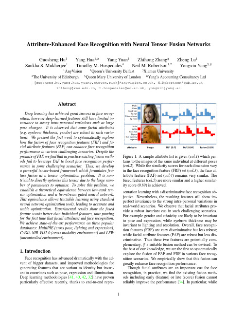
Attribute-Enhanced Face Recognition with Neural Tensor Fusion Networks Guosheng Hu1Yang Hua1,2Yang Yuan1Zhihong Zhang3Zheng Lu1 Sankha S.Mukherjee1Timothy M.Hospedales4Neil M.Robertson1,2Yongxin Yang5,61AnyVision2Queen’s University Belfast3Xiamen University 4The University of Edinburgh5Queen Mary University of London6Yang’s Accounting Consultancy Ltd {guosheng.hu,yang.hua,yuany,steven,rick}@,N.Robertson@ zhihong@,t.hospedales@,yongxin@yang.acAbstractDeep learning has achieved great success in face recog-nition,however deep-learned features still have limited in-variance to strong intra-personal variations such as large pose changes.It is observed that some facial attributes (e.g.eyebrow thickness,gender)are robust to such varia-tions.We present thefirst work to systematically explore how the fusion of face recognition features(FRF)and fa-cial attribute features(FAF)can enhance face recognition performance in various challenging scenarios.Despite the promise of FAF,wefind that in practice existing fusion meth-ods fail to leverage FAF to boost face recognition perfor-mance in some challenging scenarios.Thus,we develop a powerful tensor-based framework which formulates fea-ture fusion as a tensor optimisation problem.It is non-trivial to directly optimise this tensor due to the large num-ber of parameters to optimise.To solve this problem,we establish a theoretical equivalence between low-rank ten-sor optimisation and a two-stream gated neural network. This equivalence allows tractable learning using standard neural network optimisation tools,leading to accurate and stable optimisation.Experimental results show the fused feature works better than individual features,thus proving for thefirst time that facial attributes aid face recognition. We achieve state-of-the-art performance on three popular databases:MultiPIE(cross pose,lighting and expression), CASIA NIR-VIS2.0(cross-modality environment)and LFW (uncontrolled environment).1.IntroductionFace recognition has advanced dramatically with the ad-vent of bigger datasets,and improved methodologies for generating features that are variant to identity but invari-ant to covariates such as pose,expression and illumination. Deep learning methodologies[41,40,42,32]have proven particularly effective recently,thanks to end-to-endrepre-Figure1:A sample attribute list is given(col.1)which per-tains to the images of the same individual at different poses (col.2).While the similarity scores for each dimension vary in the face recognition feature(FRF)set(col.3),the face at-tribute feature(FAF)set(col.4)remains very similar.The fused features(col.5)are more similar and a higher similar-ity score(0.89)is achieved.sentation learning with a discriminative face recognition ob-jective.Nevertheless,the resulting features still show im-perfect invariance to the strong intra-personal variations in real-world scenarios.We observe that facial attributes pro-vide a robust invariant cue in such challenging scenarios.For example gender and ethnicity are likely to be invariant to pose and expression,while eyebrow thickness may be invariant to lighting and resolution.Overall,face recogni-tion features(FRF)are very discriminative but less robust;while facial attribute features(FAF)are robust but less dis-criminative.Thus these two features are potentially com-plementary,if a suitable fusion method can be devised.To the best of our knowledge,we are thefirst to systematically explore the fusion of FAF and FRF in various face recog-nition scenarios.We empirically show that this fusion can greatly enhance face recognition performance.Though facial attributes are an important cue for face recognition,in practice,wefind the existing fusion meth-ods including early(feature)or late(score)fusion cannot reliably improve the performance[34].In particular,while 1offering some robustness,FAF is generally less discrimina-tive than FRF.Existing methods cannot synergistically fuse such asymmetric features,and usually lead to worse perfor-mance than achieved by the stronger feature(FRF)only.In this work,we propose a novel tensor-based fusion frame-work that is uniquely capable of fusing the very asymmet-ric FAF and FRF.Our framework provides a more powerful and robust fusion approach than existing strategies by learn-ing from all interactions between the two feature views.To train the tensor in a tractable way given the large number of required parameters,we formulate the optimisation with an identity-supervised objective by constraining the tensor to have a low-rank form.We establish an equivalence be-tween this low-rank tensor and a two-stream gated neural network.Given this equivalence,the proposed tensor is eas-ily optimised with standard deep neural network toolboxes. Our technical contributions are:•It is thefirst work to systematically investigate and ver-ify that facial attributes are an important cue in various face recognition scenarios.In particular,we investi-gate face recognition with extreme pose variations,i.e.±90◦from frontal,showing that attributes are impor-tant for performance enhancement.•A rich tensor-based fusion framework is proposed.We show the low-rank Tucker-decomposition of this tensor-based fusion has an equivalent Gated Two-stream Neural Network(GTNN),allowing easy yet effective optimisation by neural network learning.In addition,we bring insights from neural networks into thefield of tensor optimisation.The code is available:https:///yanghuadr/ Neural-Tensor-Fusion-Network•We achieve state-of-the-art face recognition perfor-mance using the fusion of face(newly designed‘Lean-Face’deep learning feature)and attribute-based fea-tures on three popular databases:MultiPIE(controlled environment),CASIA NIR-VIS2.0(cross-modality environment)and LFW(uncontrolled environment).2.Related WorkFace Recognition.The face representation(feature)is the most important component in contemporary face recog-nition system.There are two types:hand-crafted and deep learning features.Widely used hand-crafted face descriptors include Local Binary Pattern(LBP)[26],Gaborfilters[23],-pared to pixel values,these features are variant to identity and relatively invariant to intra-personal variations,and thus they achieve promising performance in controlled environ-ments.However,they perform less well on face recognition in uncontrolled environments(FRUE).There are two main routes to improve FRUE performance with hand-crafted features,one is to use very high dimensional features(dense sampling features)[5]and the other is to enhance the fea-tures with downstream metric learning.Unlike hand-crafted features where(in)variances are en-gineered,deep learning features learn the(in)variances from data.Recently,convolutional neural networks(CNNs) achieved impressive results on FRUE.DeepFace[44],a carefully designed8-layer CNN,is an early landmark method.Another well-known line of work is DeepID[41] and its variants DeepID2[40],DeepID2+[42].The DeepID family uses an ensemble of many small CNNs trained in-dependently using different facial patches to improve the performance.In addition,some CNNs originally designed for object recognition,such as VGGNet[38]and Incep-tion[43],were also used for face recognition[29,32].Most recently,a center loss[47]is introduced to learn more dis-criminative features.Facial Attribute Recognition.Facial attribute recog-nition(FAR)is also well studied.A notable early study[21] extracted carefully designed hand-crafted features includ-ing aggregations of colour spaces and image gradients,be-fore training an independent SVM to detect each attribute. As for face recognition,deep learning features now outper-form hand-crafted features for FAR.In[24],face detection and attribute recognition CNNs are carefully designed,and the output of the face detection network is fed into the at-tribute network.An alternative to purpose designing CNNs for FAR is tofine-tune networks intended for object recog-nition[56,57].From a representation learning perspective, the features supporting different attribute detections may be shared,leading some studies to investigate multi-task learn-ing facial attributes[55,30].Since different facial attributes have different prevalence,the multi-label/multi-task learn-ing suffers from label-imbalance,which[30]addresses us-ing a mixed objective optimization network(MOON). Face Recognition using Facial Attributes.Detected facial attributes can be applied directly to authentication. Facial attributes have been applied to enhance face verifica-tion,primarily in the case of cross-modal matching,byfil-tering[19,54](requiring potential FRF matches to have the correct gender,for example),model switching[18],or ag-gregation with conventional features[27,17].[21]defines 65facial attributes and proposes binary attribute classifiers to predict their presence or absence.The vector of attribute classifier scores can be used for face recognition.There has been little work on attribute-enhanced face recognition in the context of deep learning.One of the few exploits CNN-based attribute features for authentication on mobile devices [31].Local facial patches are fed into carefully designed CNNs to predict different attributes.After CNN training, SVMs are trained for attribute recognition,and the vector of SVM scores provide the new feature for face verification.Fusion Methods.Existing fusion approaches can be classified into feature-level(early fusion)and score-level (late fusion).Score-level fusion is to fuse the similarity scores after computation based on each view either by sim-ple averaging[37]or stacking another classifier[48,37]. Feature-level fusion can be achieved by either simple fea-ture aggregation or subspace learning.For aggregation ap-proaches,fusion is usually performed by simply element wise averaging or product(the dimension of features have to be the same)or concatenation[28].For subspace learn-ing approaches,the features arefirst concatenated,then the concatenated feature is projected to a subspace,in which the features should better complement each other.These sub-space approaches can be unsupervised or supervised.Un-supervised fusion does not use the identity(label)informa-tion to learn the subspace,such as Canonical Correlational Analysis(CCA)[35]and Bilinear Models(BLM)[45].In comparison,supervised fusion uses the identity information such as Linear Discriminant Analysis(LDA)[3]and Local-ity Preserving Projections(LPP)[9].Neural Tensor Methods.Learning tensor-based compu-tations within neural networks has been studied for full[39] and decomposed[16,52,51]tensors.However,aside from differing applications and objectives,the key difference is that we establish a novel equivalence between a rich Tucker [46]decomposed low-rank fusion tensor,and a gated two-stream neural network.This allows us achieve expressive fusion,while maintaining tractable computation and a small number of parameters;and crucially permits easy optimisa-tion of the fusion tensor through standard toolboxes. Motivation.Facial attribute features(FAF)and face recognition features(FRF)are complementary.However in practice,wefind that existing fusion methods often can-not effectively combine these asymmetric features so as to improve performance.This motivates us to design a more powerful fusion method,as detailed in Section3.Based on our neural tensor fusion method,in Section5we system-atically explore the fusion of FAF and FRF in various face recognition environments,showing that FAF can greatly en-hance recognition performance.3.Fusing attribute and recognition featuresIn this section we present our strategy for fusing FAF and FRF.Our goal is to input FAF and FRF and output the fused discriminative feature.The proposed fusion method we present here performs significantly better than the exist-ing ones introduced in Section2.In this section,we detail our tensor-based fusion strategy.3.1.ModellingSingle Feature.We start from a standard multi-class clas-sification problem setting:assume we have M instances, and for each we extract a D-dimensional feature vector(the FRF)as{x(i)}M i=1.The label space contains C unique classes(person identities),so each instance is associated with a corresponding C-dimensional one-hot encoding la-bel vector{y(i)}M i=1.Assuming a linear model W the pre-dictionˆy(i)is produced by the dot-product of input x(i)and the model W,ˆy(i)=x(i)T W.(1) Multiple Feature.Suppose that apart from the D-dimensional FRF vector,we can also obtain an instance-wise B-dimensional facial attribute feature z(i).Then the input for the i th instance is a pair:{x(i),z(i)}.A simple ap-proach is to redefine x(i):=[x(i),z(i)],and directly apply Eq.(1),thus modelling weights for both FRF and FAF fea-tures.Here we propose instead a non-linear fusion method via the following formulationˆy(i)=W×1x(i)×3z(i)(2) where W is the fusion model parameters in the form of a third-order tensor of size D×C×B.Notation×is the tensor dot product(also known as tensor contraction)and the left-subscript of x and z indicates at which axis the ten-sor dot product operates.With Eq.(2),the optimisation problem is formulated as:minW1MMi=1W×1x(i)×3z(i),y(i)(3)where (·,·)is a loss function.This trains tensor W to fuse FRF and FAF features so that identity is correctly predicted.3.2.OptimisationThe proposed tensor W provides a rich fusion model. However,compared with W,W is B times larger(D×C vs D×C×B)because of the introduction of B-dimensional attribute vector.It is also almost B times larger than train-ing a matrix W on the concatenation[x(i),z(i)].It is there-fore problematic to directly optimise Eq.(3)because the large number of parameters of W makes training slow and leads to overfitting.To address this we propose a tensor de-composition technique and a neural network architecture to solve an equivalent optimisation problem in the following two subsections.3.2.1Tucker Decomposition for Feature FusionTo reduce the number of parameters of W,we place a struc-tural constraint on W.Motivated by the famous Tucker de-composition[46]for tensors,we assume that W is synthe-sised fromW=S×1U(D)×2U(C)×3U(B).(4) Here S is a third order tensor of size K D×K C×K B, U(D)is a matrix of size K D×D,U(C)is a matrix of sizeK C×C,and U(B)is a matrix of size K B×B.By restricting K D D,K C C,and K B B,we can effectively reduce the number of parameters from(D×C×B)to (K D×K C×K B+K D×D+K C×C+K B×B)if we learn{S,U(D),U(C),U(B)}instead of W.When W is needed for making the predictions,we can always synthesise it from those four small factors.In the context of tensor decomposition,(K D,K C,K B)is usually called the tensor’s rank,as an analogous concept to the rank of a matrix in matrix decomposition.Note that,despite of the existence of other tensor de-composition choices,Tucker decomposition offers a greater flexibility in terms of modelling because we have three hyper-parameters K D,K C,K B corresponding to the axes of the tensor.In contrast,the other famous decomposition, CP[10]has one hyper-parameter K for all axes of tensor.By substituting Eq.(4)into Eq.(2),we haveˆy(i)=W×1x(i)×3z(i)=S×1U(D)×2U(C)×3U(B)×1x(i)×3z(i)(5) Through some re-arrangement,Eq.(5)can be simplified as ˆy(i)=S×1(U(D)x(i))×2U(C)×3(U(B)z(i))(6) Furthermore,we can rewrite Eq.(6)as,ˆy(i)=((U(D)x(i))⊗(U(B)z(i)))S T(2)fused featureU(C)(7)where⊗is Kronecker product.Since U(D)x(i)and U(B)B(i)result in K D and K B dimensional vectors re-spectively,(U(D)x(i))⊗(U(B)z(i))produces a K D K B vector.S(2)is the mode-2unfolding of S which is aK C×K D K B matrix,and its transpose S T(2)is a matrix ofsize K D K B×K C.The Fused Feature.From Eq.(7),the explicit fused representation of face recognition(x(i))and facial at-tribute(z(i))features can be achieved.The fused feature ((U(D)x(i))⊗(U(B)z(i)))S T(2),is a vector of the dimen-sionality K C.And matrix U(C)has the role of“clas-sifier”given this fused feature.Given{x(i),z(i),y(i)}, the matrices{U(D),U(B),U(C)}and tensor S are com-puted(learned)during model optimisation(training).Dur-ing testing,the predictionˆy(i)is achieved with the learned {U(D),U(B),U(C),S}and two test features{x(i),z(i)} following Eq.(7).3.2.2Gated Two-stream Neural Network(GTNN)A key advantage of reformulating Eq.(5)into Eq.(7)is that we can nowfind a neural network architecture that does ex-actly the computation of Eq.(7),which would not be obvi-ous if we stopped at Eq.(5).Before presenting thisneural Figure2:Gated two-stream neural network to implement low-rank tensor-based fusion.The architecture computes Eq.(7),with the Tucker decomposition in Eq.(4).The network is identity-supervised at train time,and feature in the fusion layer used as representation for verification. network,we need to introduce a new deterministic layer(i.e. without any learnable parameters).Kronecker Product Layer takes two arbitrary-length in-put vectors{u,v}where u=[u1,u2,···,u P]and v=[v1,v2,···,v Q],then outputs a vector of length P Q as[u1v1,u1v2,···,u1v Q,u2v1,···,u P v Q].Using the introduced Kronecker layer,Fig.2shows the neural network that computes Eq.(7).That is,the neural network that performs recognition using tensor-based fu-sion of two features(such as FAF and FRF),based on the low-rank assumption in Eq.(4).We denote this architecture as a Gated Two-stream Neural Network(GTNN),because it takes two streams of inputs,and it performs gating[36] (multiplicative)operations on them.The GTNN is trained in a supervised fashion to predict identity.In this work,we use a multitask loss:softmax loss and center loss[47]for joint training.The fused feature in the viewpoint of GTNN is the output of penultimate layer, which is of dimensionality K c.So far,the advantage of using GTNN is obvious.Direct use of Eq.(5)or Eq.(7)requires manual derivation and im-plementation of an optimiser which is non-trivial even for decomposed matrices(2d-tensors)[20].In contrast,GTNN is easily implemented with modern deep learning packages where auto-differentiation and gradient-based optimisation is handled robustly and automatically.3.3.DiscussionCompared with the fusion methods introduced in Sec-tion2,we summarise the advantages of our tensor-based fusion method as follows:Figure3:LeanFace.‘C’is a group of convolutional layers.Stage1:64@5×5(64feature maps are sliced to two groups of32ones, which are fed into maxout function.);Stage2:64@3×3,64@3×3,128@3×3,128@3×3;Stage3:196@3×3,196@3×3, 256@3×3,256@3×3,320@3×3,320@3×3;Stage4:512@3×3,512@3×3,512@3×3,512@3×3;Stage5:640@ 5×5,640@5×5.‘P’stands for2×2max pooling.The strides for the convolutional and pooling layers are1and2,respectively.‘FC’is a fully-connected layer of256D.High Order Non-Linearity.Unlike linear methods based on averaging,concatenation,linear subspace learning [8,27],or LDA[3],our fusion method is non-linear,which is more powerful to model complex problems.Further-more,comparing with otherfirst-order non-linear methods based on element-wise combinations only[28],our method is higher order:it accounts for all interactions between each pair of feature channels in both views.Thanks to the low-rank modelling,our method achieves such powerful non-linear fusion with few parameters and thus it is robust to overfitting.Scalability.Big datasets are required for state-of-the-art face representation learning.Because we establish the equivalence between tensor factorisation and gated neural network architecture,our method is scalable to big-data through efficient mini-batch SGD-based learning.In con-trast,kernel-based non-linear methods,such as Kernel LDA [34]and multi-kernel SVM[17],are restricted to small data due to their O(N2)computation cost.At runtime,our method only requires a simple feed-forward pass and hence it is also favourable compared to kernel methods. Supervised method.GTNN isflexibly supervised by any desired neural network loss function.For example,the fusion method can be trained with losses known to be ef-fective for face representation learning:identity-supervised softmax,and centre-loss[47].Alternative methods are ei-ther unsupervised[8,27],constrained in the types of super-vision they can exploit[3,17],or only stack scores rather than improving a learned representation[48,37].There-fore,they are relatively ineffective at learning how to com-bine the two-source information in a task-specific way. Extensibility.Our GTNN naturally can be extended to deeper architectures.For example,the pre-extracted fea-tures,i.e.,x and z in Fig.2,can be replaced by two full-sized CNNs without any modification.Therefore,poten-tially,our methods can be integrated into an end-to-end framework.4.Integration with CNNs:architectureIn this section,we introduce the CNN architectures used for face recognition(LeanFace)designed by ourselves and facial attribute recognition(AttNet)introduced by[50,30]. LeanFace.Unlike general object recognition,face recognition has to capture very subtle difference between people.Motivated by thefine-grain object recognition in [4],we also use a large number of convolutional layers at early stage to capture the subtle low level and mid-level in-formation.Our activation function is maxout,which shows better performance than its competitors[50].Joint supervi-sion of softmax loss and center loss[47]is used for training. The architecture is summarised in Fig.3.AttNet.To detect facial attributes,our AttNet uses the ar-chitecture of Lighten CNN[50]to represent a face.Specifi-cally,AttNet consists of5conv-activation-pooling units fol-lowed by a256D fully connected layer.The number of con-volutional kernels is explained in[50].The activation func-tion is Max-Feature-Map[50]which is a variant of maxout. We use the loss function MOON[30],which is a multi-task loss for(1)attribute classification and(2)domain adaptive data balance.In[24],an ontology of40facial attributes are defined.We remove attributes which do not characterise a specific person,e.g.,‘wear glasses’and‘smiling’,leaving 17attributes in total.Once each network is trained,the features extracted from the penultimate fully-connected layers of LeanFace(256D) and AttNet(256D)are extracted as x and z,and input to GTNN for fusion and then face recognition.5.ExperimentsWefirst introduce the implementation details of our GTNN method.In Section5.1,we conduct experiments on MultiPIE[7]to show that facial attributes by means of our GTNN method can play an important role on improv-Table1:Network training detailsImage size BatchsizeLR1DF2EpochTraintimeLeanFace128x1282560.0010.15491hAttNet0.050.8993h1Learning rate(LR)2Learning rate drop factor(DF).ing face recognition performance in the presence of pose, illumination and expression,respectively.Then,we com-pare our GTNN method with other fusion methods on CA-SIA NIR-VIS2.0database[22]in Section5.2and LFW database[12]in Section5.3,respectively. Implementation Details.In this study,three networks (LeanFace,AttNet and GTNN)are discussed.LeanFace and AttNet are implemented using MXNet[6]and GTNN uses TensorFlow[1].We use around6M training face thumbnails covering62K different identities to train Lean-Face,which has no overlapping with all the test databases. AttNet is trained using CelebA[24]database.The input of GTNN is two256D features from bottleneck layers(i.e., fully connected layers before prediction layers)of LeanFace and AttNet.The setting of main parameters are shown in Table1.Note that the learning rates drop when the loss stops decreasing.Specifically,the learning rates change4 and2times for LeanFace and AttNet respectively.Dur-ing test,LeanFace and AttNet take around2.9ms and3.2ms to extract feature from one input image and GTNN takes around2.1ms to fuse one pair of LeanFace and AttNet fea-ture using a GTX1080Graphics Card.5.1.Multi-PIE DatabaseMulti-PIE database[7]contains more than750,000im-ages of337people recorded in4sessions under diverse pose,illumination and expression variations.It is an ideal testbed to investigate if facial attribute features(FAF) complement face recognition features(FRF)including tra-ditional hand-crafted(LBP)and deeply learned features (LeanFace)to improve the face recognition performance–particularly across extreme pose variation.Settings.We conduct three experiments to investigate pose-,illumination-and expression-invariant face recogni-tion.Pose:Uses images across4sessions with pose vari-ations only(i.e.,neutral lighting and expression).It covers pose with yaw ranging from left90◦to right90◦.In com-parison,most of the existing works only evaluate perfor-mance on poses with yaw range(-45◦,+45◦).Illumination: Uses images with20different illumination conditions(i.e., frontal pose and neutral expression).Expression:Uses im-ages with7different expression variations(i.e.,frontal pose and neutral illumination).The training sets of all settings consist of the images from thefirst200subjects and the re-maining137subjects for testing.Following[59,14],in the test set,frontal images with neural illumination and expres-sion from the earliest session work as gallery,and the others are probes.Pose.Table2shows the pose-robust face recognition (PRFR)performance.Clearly,the fusion of FRF and FAF, namely GTNN(LBP,AttNet)and GTNN(LeanFace,At-tNet),works much better than using FRF only,showing the complementary power of facial features to face recognition features.Not surprisingly,the performance of both LBP and LeanFace features drop greatly under extreme poses,as pose variation is a major factor challenging face recognition performance.In contrast,with GTNN-based fusion,FAF can be used to improve both classic(LBP)and deep(Lean-Face)FRF features effectively under this circumstance,for example,LBP(1.3%)vs GTNN(LBP,AttNet)(16.3%), LeanFace(72.0%)vs GTNN(LeanFace,AttNet)(78.3%) under yaw angel−90◦.It is noteworthy that despite their highly asymmetric strength,GTNN is able to effectively fuse FAF and FRF.This is elaborately studied in more detail in Sections5.2-5.3.Compared with state-of-the-art methods[14,59,11,58, 15]in terms of(-45◦,+45◦),LeanFace achieves better per-formance due to its big training data and the strong gener-alisation capacity of deep learning.In Table2,2D meth-ods[14,59,15]trained models using the MultiPIE images, therefore,they are difficult to generalise to images under poses which do not appear in MultiPIE database.3D meth-ods[11,58]highly depend on accurate2D landmarks for 3D-2D modellingfitting.However,it is hard to accurately detect such landmarks under larger poses,limiting the ap-plications of3D methods.Illumination and expression.Illumination-and expression-robust face recognition(IRFR and ERFR)are also challenging research topics.LBP is the most widely used handcrafted features for IRFR[2]and ERFR[33].To investigate the helpfulness of facial attributes,experiments of IRFR and ERFR are conducted using LBP and Lean-Face features.In Table3,GTNN(LBP,AttNet)signifi-cantly outperforms LBP,80.3%vs57.5%(IRFR),77.5% vs71.7%(ERFR),showing the great value of combining fa-cial attributes with hand-crafted features.Attributes such as the shape of eyebrows are illumination invariant and others, e.g.,gender,are expression invariant.In contrast,LeanFace feature is already very discriminative,saturating the perfor-mance on the test set.So there is little room for fusion of AttrNet to provide benefit.5.2.CASIA NIR-VIS2.0DatabaseThe CASIA NIR-VIS2.0face database[22]is the largest public face database across near-infrared(NIR)images and visible RGB(VIS)images.It is a typical cross-modality or heterogeneous face recognition problem because the gallery and probe images are from two different spectra.The。
A Comprehensive Survey of Multiagent Reinforcement Learning
IEEE TRANSACTIONS ON SYSTEMS, MAN, AND CYBERNETICS—PART C: APPLICATIONS AND REVIEWS, VOL. 38, NO. 2, MARCH 2008
A Comprehensive Survey of Multiagent ReinfoN
A
MULTIAGENT system [1] can be defined as a group of autonomous, interacting entities sharing a common environment, which they perceive with sensors and upon which they act with actuators [2]. Multiagent systems are finding applications in a wide variety of domains including robotic teams, distributed control, resource management, collaborative decision support systems, data mining, etc. [3], [4]. They may arise as the most natural way of looking at the system, or may provide an alternative perspective on systems that are originally regarded as centralized. For instance, in robotic teams, the control authority is naturally distributed among the robots [4]. In resource management, while resources can be managed by a central authority, identifying each resource with an agent may provide a helpful, distributed perspective on the system [5].
- 1、下载文档前请自行甄别文档内容的完整性,平台不提供额外的编辑、内容补充、找答案等附加服务。
- 2、"仅部分预览"的文档,不可在线预览部分如存在完整性等问题,可反馈申请退款(可完整预览的文档不适用该条件!)。
- 3、如文档侵犯您的权益,请联系客服反馈,我们会尽快为您处理(人工客服工作时间:9:00-18:30)。
a r X i v :h e p -p h /0507295v 2 23 D e c 2005Factorization and polarization in two charmed-mesonB decaysChuan-Hung Chen a,d ∗,Chao-Qiang Geng b †and Zheng-Tao Wei c,d‡a Department of Physics,National Cheng-Kung University,Tainan,701TaiwanbDepartment of Physics,National Tsing-Hua University,Hsin-Chu,300TaiwancInstitute of Physics,Academia Sinica,Taipei,115TaiwandNational Center for Theoretical Sciences,TaiwanAbstractWe provide a comprehensive test of factorization in the heavy-heavy B decays motivated by the recent experimental data from BELLE and BABAR collaborations.The penguin effects are not negligible in the B decays with two pseudoscalar mesons.The direct CP asymmetries are found to be a few percent.We give estimates on the weak annihilation contributions by analogy to the observed annihilation-dominated processes.The N c insensitivity of branching ratios indicates thatthe soft final state interactions are not dominant.We also study the polarizations in B →D ∗D ∗(s )decays.The power law shows that the transverse perpendicular polarization fraction is small.The effects of the heavy quark symmetry breaking caused by the perturbative QCD and power corrections on the transverse polarization are also investigated.I.INTRODUCTIONThe study of B meson weak decays is of high interest in heavyflavor physics and CP violation.In particular,much attention has been paid to the two-body charmless hadronic B decays,but there are relatively less discussions on the decays with charmful mesons,such as the modes with two charmed-meson in which thefinal states are both heavy.However, the two charmed-meson decays can provide some valuable and unique information which is different from the light meson productions.For example,CP asymmetries in the decays of B→D(∗)+D(∗)−play important roles in testing the consistency of the standard model (SM)as well as exploring new physics[1].Moreover,these decays are ideal modes to check the factorization hypothesis as the phenomenon of color transparency for the light energetic hadron is not applicable.Since the decay branching ratios(BRs),CP asymmetries(CPAs) and polarizations of B→D(∗)D(∗)(D(∗)D(∗)s)have been partially observed in experiments [2,3,4],it is timely to examine these heavy-heavy B decays in more detail.At the quark level,one concludes that the two charmed-meson decays are dominated by tree contributions since the corresponding inclusive modes are b→qc¯c with q=s and d.It is known that the factorization has been tested to be successful in the usual color-allowed processes.However,the mechanism of factorization in heavy-heavy decays is not the same as the case of the light hadron productions.The color transparency argument[5]for light energetic hadrons is no longer valid to the modes with heavy-heavyfinal states.The reason can be given as follows.Due to the intrinsic soft dynamics in the charmed-meson,non-vanishing soft gluon contributions are involved in the strong interactions between an emission heavy meson with the remained BD(∗)system.Since the corresponding divergences may not be absorbed in the definition of the hadronic form factor or hadron wave function,the decoupling of soft divergences is broken.This means that the mechanism of factorization has to be beyond the perturbative frameworks,such as QCD factorization[6]and soft-collinear effective theory[7].The large N c limit is another mechanism to justify factorization[8], corresponding to the effective color number N c=∞in the naive factorization approach [9].The understanding of factorization in heavy-heavy decays requires some quantitative knowledge of non-perturbative physics which is not under control in theory.In this paper, we will assume the factorization hypothesis and apply the generalized factorization approach (GFA)[10,11]to calculate the hadronic matrix elements.It is known that annihilation contributions and nonfactorizable effects withfinal state interactions(FSIs)play important role during the light meson production in B meson decays. For instance,to get large strong phases for CP asymmetries(CPAs)in B→Kπand B→ππdecays,these effects are included inevitably[12,13].Moreover,they are also crucial to explain the anomaly of the polarizations in B→φK∗decays,measured by BABAR[14] and BELLE[15]recently.By the naive analysis inflavor diagrams,one can easily see thatthe decay modes of B→D(∗)0¯D(∗)0and D(∗)0s ¯D(∗)0sare annihilation-dominated processes.Therefore,measurements of these decays will clearly tell us the importance of annihilation contributions in the production of two charmed-meson modes.For the color-allowed decays,since the short-distant(SD)nonfactorizable parts are as-sociated with the Wilson coefficient(WC)of C1/N c,where C1is induced by the gluon-loop and it is much smaller than C2∼1,we can see that the effects arising from the SD non-spectator contributions should be small[16].Nevertheless,long-distant(LD)nonfactorizable contributions governed by rescattering effects or FSIs may not be negligible.Inspired by the anomaly of the large transverse perpendicular polarization,denoted by R⊥,in B→φK∗decays,if there exist significant LD effects,we believe that large values of R⊥may appear in B→D∗D∗and B→D∗D∗s too.As we will discuss,the power-law in the two-vector charmed-meson decay leads to a small R⊥.The recent measurement of the polarization fraction by the BELLE collaboration gives R⊥=0.19±0.08±0.01[3]in which the central value is about a factor of three comparing with the model-independent prediction within the factorization approach and heavy quark symmetry.Clearly,to get the implication from the data,we need a detailed analysis in two charmfulfinal states of B decays.To estimate the relevant hadronic effects for two-body decays in the B system,we use the GFA,in which the leading effects are factorized parts,while the nonfactorized effects are lumped and characterized by the effective number of colors,denoted by N effc.Note that the scale and scheme dependences in effective WCs C effi are insensitive.In the framework of the GFA,since the formulas for decay amplitudes are associated with the transition form factors,we consider them based on heavy quark effective theory(HQET)[17].We will also study theirαs[18]and power corrections which break heavy quark symmetry(HQS)[19]. In our analysis,we will try tofind out the relationship between the HQS and its breaking effects for R⊥.In addition,we will reexamine the influence of penguin effects,neglected in the literature[20].We will show that sizable CPAs in¯B0→D+D−and B−→D0D−decays may rely on FSIs.This paper is organized as follows.In Sec.II,we give the effective Hamiltonian for the heavy-heavy B decays.The definition of heavy-to-heavy form factors are also introduced.In Sec.III,we show the general formulas for B to two charmful states in the framework of the GFA.The effects of the heavy quark symmetry breaking on the transverse perpendicular polarization are investigated.In Sec.IV,we provide the numerical predictions on the BRs,direct CPAs and the polarization fractions.Conclusions are given in Sec.V.We collect all factorized amplitudes for B →P P,P V (V P )and V V decays in Appendixes.II.EFFECTIVE INTERACTIONS AND PARAMETRIZATION OF FORM F AC-TORSThe relevant effective Hamiltonian for the B meson decaying to two charmful meson states is given by [21],H eff(∆B =1)=G F 2V ub V ∗uq [C 1(µ)O u 1+C 2(µ)O u 2]+V cb V ∗cq [C 1(µ)O c 1+C 2(µ)O c2]−V tb V ∗tq10k =3C k (µ)O k +H.c.,(1)where q =s and d ,V ij denote the Cabibbo-Kobayashi-Masikawa (CKM)matrix elements,C i (µ)are the Wilson coefficients (WCs)and O i are the four-fermion operators,given byO u1=(¯q i u j )V −A (¯u j b i )V −A ,O u2=(¯q i u i )V −A (¯u j b j )V −A ,O c 1=(¯q i c j )V −A (¯c j b i )V −A ,O c 2=(¯q i c i )V −A (¯c j b j )V −A ,O 3(5)=(¯q i b i )V −Aq ′(¯q ′j q ′j )V ∓A ,O 4(6)=(¯q i b j )V −Aq ′(¯q ′j q ′i )V ∓A ,O 7(9)=32(¯q i b j )V −Aq ′e q ′(¯q ′j q ′i )V ±A .(2)with i and j being the color indices,O 3−6(O 7−10)the QCD (electroweak)penguin operators and (¯q 1q 2)V ±A =¯q 1γµ(1±γ5)q 2.In order to cancel the renormalization scale and scheme dependence in the WCs of C i (µ),the effective WCs are introduced byC (µ) O (µ) ≡C eff O tree .(3)Since the matrix element O tree is given at tree level,the effective WCs are renormalization scale and scheme independent.To be more useful,we can define the effective WCs asa eff1=C eff2+C eff1(N effc)2,a eff(q) 3,4=C eff3,4+C eff4,32e q C eff9,10+C eff10,9(N effc)6,5+3(N effc)8,7 ,(4)where1N c+χi.(5) withχi being the non-factorizable terms.In the GFA,1/(N effc)i are assumed to be universal and real in the absence of FSIs.In the naive factorization,all effective WCs C effi are reduced to the corresponding WCs of C i in the effective Hamiltonian and the non-factoziable terms are neglected,i.e.,χi=0.Under the factorization hypothesis,the tree level hadronic matrix element O tree is fac-torized into a product of two matrix elements of single currents,which are represented by the decay constant and form factors.The B→H(H=D,D∗)transition form factors are crucial ingredients in the GFA for the heavy-heavy decays.To obtain the transition elements of B→H with various weak vertices,wefirst parameterize them in terms of the relevant form factors under the conventional forms as follows:D|Vµ|¯B =F1(q2) Pµ−P·q q2F0(q2)qµ,(6) D∗(ǫ)|Vµ|¯B =V(q2)q2qµ+(m B+m D∗)A1(q2) ǫ∗µ−ǫ∗·qm B+m D∗ Pµ−P·qfound in Ref.[19]and the relation with the conventional ones are given byF1(q2)=m B+m Dm B m D ξ+(w)−m B−m D2√m B−m Dw−1 2√2√2√m BξA2(w),A3(q2)=m B+m D∗m B m D∗ m B2m D∗ ξA3(w)+m D∗4m B m D∗ m D∗ξA3(w)−m D∗m2+m3f P2m2B−m2P1motion for on-shell quarks.Moreover,we use X (BP,V )1≡ V |(¯q 2q 3)V −A |0 P |(¯q 1b )V −A |¯B =2f V m V F BP 1(m 2V )(ε∗·p B),X (BV,P )1≡ P |(¯q 2q 3)V −A |0 V |(¯q 1b )V −A |¯B =2f P m V A BV 0(m 2P )(ε∗·p B ),X (BV,P )2≡ P |(¯q 2q 3)S +P |0 V |(¯q 1b )S −P |¯B =2m 2P m b +m 1A BV 0(m 2P )(ε∗·pB ),(10)andX (BV 1,V 2)≡ V 2|(¯q 2q 3)V −A |0 V 1|(¯q 1b )V −A |¯B=−if V 2m V 2(ε∗1·ε∗2)(m B+m V 1)A BV 11(m 2V 2)−(ǫ∗1·p 2)(ǫ∗2·p 1)2A BV 12(m 2V 2)(m B +m V 1),(11)for B →P V (V P )and B →V V ,respectively.We note that the sign difference ofX (BP 1,P 2)1and X (BP 1,P 2)2in Eq.(9)will make the penguin effects become non-negligible.On the other hand,the same sign of X (BV,P )1and X (BV,P )2in Eq.(10)leads to thepenguin effects negligible.Since the time-like form factors for annihilation contributions are uncertain,we take Y (B,M 1M 2)1(2)≡ M 1M 2|(¯q 2q 3)V ∓A |0 0|(¯q 1b )V −A |¯Band Y (B,M 1M 2)3≡ M 1M 2|(¯q 2q 3)S +P |0 0|(¯q 1b )S −P |¯Bto represent them,where M can be pseudoscalar or vec-tor bosons.Note that due to the identity of εi (p i )·p i =0,we have used V |(¯q 2q 3)S +P |0 =0.With these notations and associated effective WCs,one can display the decay amplitude for the specific decay mode.We summary the relevant decay amplitudes in Appendixes.Once we get the decay amplitude,denoted by A (B →M 1M 2),the corresponding decay rate of the two-body mode could be obtained byΓ(B →M 1M 2)=G F p¯Γ(¯B →¯M 1¯M 2)+Γ(B →M 1M 2).(13)Besides the BRs and CPAs,we can also study the polarizations of the vector mesons in B →V V decays.To discuss the polarizations,one can write the general decay amplitudes in the helicity basis to beA (λ)=ǫ∗1µ(λ)ǫ∗2ν(λ)a gµν+bm V 1m V 2ǫµναβp 1αp 2β.(14)In this basis,the amplitudes with various helicities can be given asH0=−ax−b(x2−1),H±=a±√√2a,A⊥=12(H+−H−)=√x2−1c.(15)Accordingly,the decay rate expressed by helicity amplitudes for the VV mode can be written asΓ=G F p|A0|2+|A |2+|A⊥|2.(16) where i=0and (⊥),representing the longitudinal and transverse parallel(perpendicular) components,respectively,with the relation of R0+R +R⊥=1.Under CP parities,R0, are CP-even while R⊥is CP-odd.From the hadronic matrix element in Eq.(11),the amplitudes a,b and c in the framework of the GFA are expressed bya=−˜C eff(m B+m V1)m V2f V2A BV11(m2V2),b=˜C eff 2m V1m2V2m B+m V1f V2V BV1(m2V2).(17)where˜C eff represents the involved WCs and CKM matrix elements.With the form factors in Eq.(8)and the heavy quark limit,we get that the ratios r b=b/a and r c=c/a are related.Explicitly,we haver b=r c=m D∗(1+w)≈0.16,(18)which are small.From Eqs.(15)and(16),wefind that the polarization fractions behave asR0∼R ,R⊥∼O m2D∗which indicate that the power law in the heavy-heavy decays is different from the light-light ones,which are expected to be R0∼1,R ∼R⊥∼O(m2V/m2B).Moreover,R⊥is directlyrelated to c and can be written as1R⊥=≈ ζD∗V(q2)R HQS⊥and D+s D−s modes,the four modes have the same decay topologies.Hence,by assuming that they have similar hadronic effects,the BRs of B0→D0¯D0(D+s D−s)could be estimated tobe less than O(10−6).To give a detailed analysis,we can include the character of each mode,governed by the meson distribution amplitudes.For simplicity,we will concentrate on the leading twist effects and take the meson wave functions to beΦD∝f D x(1−x)(1+0.8(1−2x))[23],ΦD s∝f D s x(1−x)(1+0.3(1−2x))[24],J/Ψ∝f J/Ψx(1−x)(x(1−x)/(1−2.8x(1−x)))0.7 [25]andΦK∝f K x(1−x)(1+0.51(1−2x)+0.3[5(1−2x)2−1])[26],where x is the momentum fraction of the parton inside the meson and f D,D s,J/Ψ,K are the decay constants of D,D s,J/Ψand K mesons,respectively.From these wave functions,we know that the maximum contributions are from x0≈(0.35,0.43,0.5,0.5)for(D,D s,J/Ψ,K).With the information,we can estimate the decay amplitudes in order of magnitude for¯B d→D+s K−(J/ΨD0)and¯B d→D0¯D0(D+s D−s)as shown in Figs.1a and1b with q′=s(c)and q=u(s),respectively.Note that there exists a chiral suppression in the factorized parts in annihilation contributions.However,we just consider the nonfactorized effects in the estimations.Therefore,by Fig.1with the gluon exchange,the decay amplitude is related to the propagators of the gluon and the light quark,described by1/(k2+k3)2/(k2+k3)2, where k2(3)denote the momenta carried by the spectators.For simplicity,we have neglected the momentum carried by the light quark of the B meson.By the momentum fraction,the decay amplitude could satisfy that A∝1/(x2x3)2.Hence,the relative size of the decay amplitudes could be given approximately asA(D+s K−):A(J/ΨD0):A(D0¯D0):A(D+s¯D−s)∼f D s f K(x2x3)2:λf2D(x2x3)2.With the information of maximum contributions,characterized by x0for each mode,we get A(D+s K−):A(J/ΨD0):A(D0¯D0):A(D+s¯D−s)∼1:f D f J/Ψ0.65 2:λf2D0.3522:λf D s0.43 2.(22)With the kinetic effects,the ratios of BRs are roughly to be BR(D+s K−):BR(J/ΨD0): BR(D0¯D0):BR(D+s¯D−s)∼1:0.25:0.39:0.16.That is,the BRs of¯B→D0¯D0(D+s D−s) could be as large as O(10−6),which implies that annihilation effects could be neglected in the discussions on the BR of the production for color-allowed two charmful mesons.We note that our estimations are just based on SD effects and at the level of order of magnitude. Clearly,direct experimental measurements are needed to confirm our results.B.αs,power corrections and the parametrization of Isgur-Wise functionIn the HQS limit,the form factors could be related to a single Isgur-Wise functionξ(ω)byξ+=ξV=ξA1=ξA3=ξ(w)andξ−=ξA2=0.We now include the perturbativeQCD corrections induced by hard gluon vertex corrections of b→c transitions and power corrections in orders of1/m Q with Q=b and c.Consequently,the form factors can be written asξi(w)={αi+βi(w)+γi(w)}ξ(w).(23)whereξ(w)is the Isgur-Wise function,α+=αV=αA1=αA3=1,α−=αA2=0andβi(ω)andγi(ω)stand for effects ofαs and power corrections,respectively.Explicitly,for the two-body decays in our study,ω∼1.3and the values of the other parameters are summarized as follows[18,19]:β+=−0.043,β−=0.069,βV=0.072,βA1=−0.067,βA2=−0.114,βA3=−0.028,γ+=0.015,γ−=−0.122,γV=0.224,γA1=0.027,γA2=−0.093,γA3=0.014.(24)Clearly,the range of their effects is from few percent to20%level.In particular,the power corrections to the form factorξV(or say V(q2))are the largest,about20%.The resultant is also consistent with other QCD approaches,such as the constitute quark model(CQM) [27]and the light-front(LF)QCD[28].After taking care of the corrections,the remaining unknown is the Isgur-Wise function.To determine it,we adopt a linear parametrization to beξ(w)=1−ρ2H(w−1)for the transition B→H,whereρ2H is called the slope parameter.We use the BRs of semileptonic B→D(∗)ℓ−¯νℓdecays to determineρ2H.We note that the values ofρ2D andρ2D∗are not the same as those in D and D∗decays.In our approach,the difference is from higher orders and power corrections.Hence,with V cb=0.0416and BR(B→D(∗)ℓ−¯νℓ)=2.15±0.22(6.5±0.5)%[2], we obtainρ2D=0.90±0.06andρ2D∗=1.09±0.05.Since the errors ofρ2H are small,we will only use the central values in our numerical results.C.Results for BRs and polarization fractionsTo get the numerical estimations,the input values for the relevant parameters are taken to be as follows[2,29,30]:f D=0.20,f D∗=0.23,f D s=0.24,f D∗s=0.275GeV;V cd=−λ,V cs=1−λ2/2,V cb=Aλ2,V td=λ|V cb|R t e−iφ1,V ts=−Aλ2,V tb=1,A=0.83,λ=0.224,φ1=23.4o,R t=0.91;m u=0.005,m d=0.01,m s=0.15,m c=1.5,m b=4.5GeV.(25)Note that the numerical results are insensitive to light quark masses.As to the WCs,we adopt the formulas up to one-loop corrections presented in Ref.[11]and setµ=2.5GeV. As mentioned early,since the nonfactorized contributions are grouped into N effc,the color number in Eq.(4)will be regarded as a variable.To display their effects,we take the values of N effc=2,3,5and∞.By following the factorized formulas shown in Appendixes,we present the BRs with various N effc in Tables I,II and III for P P,P V(V P)and V V modes,respectively.In order to accord with the experimental data,our predictions of the BRs are given as the CP-averaged values.For comparisons,we also calculate the results in terms of the form factors given by the CQM and LF,which are displayed in Table IV.Since the CPAs are quite similar in different models,in Table IV we just show the results in our approach.As to the polarization fractions,we present them in Table V.Therein,to understand the influence of the HQS breaking effects,we separate the results to be HQS and HQS I(II),representing the HQS results and those withαs(αs+power)corrections,respectively.TABLE I:BRs(in unit of10−3)for B→P P decays withρ2D=0.90.mode N effc=2N effc=3N effc=5N effc=∞Exp.B−→D0D−s7.858.949.8211.3413±4[2]B−→D0D−0.300.330.370.430.562±0.082±0.065[3]TABLE II:BRs(in unit of10−3)for B→P V(V P)decays withρ2=0.90(1.09).D(∗)mode N effc=2N effc=3N effc=5N effc=∞Exp.¯B0→D∗+D−s 6.787.678.419.6610.7±2.9[2]B−→D∗0D−s7.378.349.1410.4912±5[2]¯B0→D+D∗−0.370.420.460.53B−→D0D∗−0.400.450.500.570.459±0.072±0.056[3]¯B0→D∗+D∗−s22.5225.5127.9832.1919±5[2];18.8±0.9±1.7[4]¯B0→D∗+D∗−0.870.910.99 1.140.81±0.08±0.11[3];0.87±0.18[2]TABLE IV:BRs(in unit of10−3)with N effc=3and the form factors calculated in the CQM,LF and HQSC,while the CPA is only shown in our approach(HQSC).Mode CQM LF HQSC A CP(%) B−→D0D−s10.5811.268.94−0.2 B−→D0D−0.420.440.332.5¯B0→D+D∗−s12.4911.4210.80−0.1 B−→D0D∗−s13.6512.4711.73−0.1¯B0→D∗+D−0.360.330.290.2¯B0→D∗+D−0.730.780.710.6 +D+D∗−B−→D∗0D−0.390.360.310.2¯B0→D∗+D∗−s28.7827.0925.51−0.1¯B0→D∗+D∗− 1.060.990.910.9TABLE V:Polarization fractions in various QCD approaches,where HQS I and HQS II denote the results withαs andαs+power corrections,respectively.Mode CQM LF HQS HQS I HQS II B−→D∗0D∗−s R0=0.524R0=0.512R0=0.515R0=0.517R0=0.512 R⊥=0.070R⊥=0.078R⊥=0.055R⊥=0.070R⊥=0.093 B−→D∗0D∗−R0=0.547R0=0.535R0=0.538R0=0.541R0=0.535 R⊥=0.069R⊥=0.077R⊥=0.055R⊥=0.070R⊥=0.092 the branching ratio is BR(our result)× f D ssame as those in the V V modes due to the vector meson being factorized out from theB→P transition.Since the WCs a eff(c)4and a eff(c)6have the same sign,we see clearly thatpenguin effects in the P P modes are larger than those in the V V modes;however,due tothe cancelation between a eff(c)4and a eff(c)6,penguin effects could be neglected in B→V Pdecays.Hence,the ratios|P/T|for P P,V P and V V(P V))are around15%,0%and4%, respectively.For the P P,V V(P V)modes,our predictions are consistent with the results in Refs.[31,32].Note that an4%penguin contribution was obtained for the V P modes in [31].The difference is due to that they used a lower charm quark mass(m c=0.95GeV) than ours.For all the decay modes,the electroweak penguin contributions can be negligible (less than1%).(4)Without FSIs,wefind that the BRs in the neutral and charged modes have the following relationships:1τB+BR(D(∗)0D(∗)−s),1τB+BR(D(∗)0D(∗)−).In addition,the decays with nonstrangeness charmed mesons are Cabibbo-suppressed com-pared to the decays with the D(∗)s emission and they satisfyBR(B→D(∗)D(∗))≈f2 D(∗)1+(P/T)2+2(P/T)cosδcosθW.(28) According to the discussions in(1),the maximum CPAs in P P,P V and V V(V P)are expected to be around26%,0%and8%,respectively.However,in B→D(∗)D(∗)decays,dueto|θW|=|φ1|,if we takeδ=90o andφ=23.4o,the maximum CPAs for P P and V V(V P) modes are10.3%and1.6%,respectively.Clearly,in the SM,the CPA with O(10%)can be reached in B→DD decays.Due to the associated CKM matrix element being V ts≈−Aλ2, there are no CPAs in B→D(∗)D(∗)s decays.In the GFA,since the strong phases mainly arise from the one-loop corrections which are usually small,our results on CPAs,shown in Table IV,are all at a few percent level.Therefore,if the CPAs of O(10%)are found in ¯B0→D+D−and¯B+→D0D−decays,we can conclude the large effects of the strong phase are from FSIs.(6)As discussed before,we know that in two charmful decays the polarization fractions satisfy R⊥<<R0∼R .The current experimental data are:R0=0.52±0.05[2]for B0→D∗+D∗−s and R0=0.57±0.08±0.02,R⊥=0.19±0.08±0.01[3]and R⊥=0.063±0.055±0.009 [4]for B0→D∗+D∗−.We can see that the experimental measurements support the power-law relation.To estimate how large R⊥can be in theory,we use the relationship in Eq.(21) and the form factors in Eq.(7)and we obtainR⊥1+βA1+γA12.(29)With the values in Eq.(24)and R HQS⊥=0.055,we get R⊥≈10%.The detailed numerical values can be found in Table V.Interestingly,for the¯B0→D∗+D∗−decay,the estimated result is close to the upper limit of R⊥=0.063±0.055±0.009observed by BABAR[4]but close to the lower limit of R⊥=0.19±0.08±0.01observed by BELLE[3].We note that our results are different from the PQCD predictions in which R⊥∼0.06[16].From our results, we can conjecture that if large R⊥,say around20%,is observed,large contributions should arise from FSIs.V.CONCLUSIONSWe have presented a detailed study of B decaying into two charmed-mesons in the gener-alized factorization approach.The penguin contributions have also been taken into account. If thefinal states are both pseudoscalar mesons,the ratio of penguin and tree contributions is about10%in the decay amplitude.The direct CP violating asymmetries have been esti-mated to be a few percent.For the B0→D∗+D−,D+D∗−,D∗+D∗−decays,the“penguin pollution”is weaker than that in the D+D−mode.Thus,these modes provide cleaner placesto cross-check the value of sin2βmeasured in the B0→J/ψK decays.The weak annihila-tion contributions have been found to be small.We have proposed to test the annihilation effects in annihilation-dominated processes of B0→D(∗)0¯D(∗)0and D(∗)+s D(∗)−s.We have performed a comprehensive test of the factorization in the heavy-heavy B decays. The predictions of branching ratios in theory are consistent with the experimental data within the present level.The variations of branching ratios with the effective color number N effc show that the soft FSIs are not dominant.However,we cannot make the conclusion that they are negligible.Their effects can be of order10-20%for branching ratios as indicated from the variation of N effc.Since the soft divergences are not canceled in the non-factorizable corrections,this may indicate that the strong interactions at low energy either become weak or are suppressed by some unknown parameters(such as N c in the large N c theory).If the factorization is still a working concept in the heavy-heavy decays,there must be some non-perturbative mechanisms which prefer the factorization of a large-size charmed-meson from an environment of“soft cloud”.A relevant comment on the necessity of non-perturbative QCD justification can be found in[34].The polarization structure in the heavy-heavy decays has shown that the transverse perpendicular polarization fraction R⊥is the smallest while the other two are comparable in size.This structure follows from the QCD dynamics in the heavy quark limit.We have found one relation between the transverse perpendicular polarization fraction and the ratios of form factors,in particular V(q2)/A1(q2).The corrections to the heavy quark limit give an enhancement of R⊥from0.055to about0.09.Since the FSIs are not significant,we do not expect that FSIs can change our prediction of R⊥substantially.If future measurements confirm R⊥∼0.2as the recent measurement by BELLE,it will be difficult to explain within the HQET and the factorization hypothesis.In conclusion,our study has shown that the factorization works well in B meson heavy-heavy decays at present.More precise experimental data are desired to give a better jus-tification.For theory,to explain the mechanism of factorization in the heavy-heavy decays is of high interest.The measurement of the transverse perpendicular polarization provides important information on the size of the heavy quark symmetry breaking or the possibility of large non-factorizable effects.AcknowledgmentsWe thank Hai-Yang Cheng and Yu-Kuo Hsiao for many valuable discussions.This work is supported in part by the National Science Council of R.O.C.under Grant #s:NSC-93-2112-M-006-010and NSC-93-2112-M-007-014.B →P P DECAYSA (¯B 0→D +D −s )=V cb V ∗cs a eff1X (BD,D s )1−V tb V ∗tsa eff(c)4X (BD,D s )1−2a eff(c)6X (BD,D s )2 + a eff(d)4Y (B,DD s )1−2a eff(d)6Y (B,DD s )3 ,(30)A (¯B 0→D +s D −s )=V cb V ∗cd a eff2Y (B,D s D s )1−V tb V ∗td(a eff(s)3+a eff(c)3)Y (B,D s D s)1+(a eff(s)5+a eff(c)5)Y (B,D s D s )2,(31)A (B −→D0D −s )=V cb V ∗cs a eff1X (BD,D s )1+V ub V ∗us a eff1Y (B,DD s )1−V tb V ∗tsa eff(c)4X (BD,D s )1−2a eff(c)6X (BD,D s )2+a eff(u)4Y (B,DD s )1−2a eff(u)6Y (B,DD s )3 ,(32)A (¯B 0→D +D −)=V cb V ∗cda eff1X (BD,D )1+a eff2Y (B,DD )1 −V tb V ∗td a eff(c)4X (BD,D )1−2a eff(c)6X (BD,D )2+(a eff(d)4+a eff(d)3+a eff(c)3)Y (B,DD )1+(a eff(d)5+a eff(c)5)Y (B,DD )2−2a eff(d)6Y (B,DD )3,(33)A (¯B 0→D 0¯D 0)=(V cb V ∗cd +V ub V ∗ud )a eff2Y (B,DD )1−V tb V ∗td(a eff(u)3+a eff(c)3)Y (B,DD )1+(a eff(u)5+a eff(c)5)Y (B,DD )2,(34)A (B −→D 0D −)=V cb V ∗cda eff1X (BD,D )1+V ub V ∗uda eff1Y (B,DD )1−V tb V ∗tda eff(c)4X (BD,D )1−2a eff(c)6X (BD,D )2 +a eff(d)4Y (B,DD )1−2a eff(d)6Y (B,DD )3.(35)。