Matlab Simulation for BUS Suspension System
汽车动力性试验仿真matlab

汽车动⼒性试验仿真matlab基于matlab 的⼀款轻型货车动⼒性试验仿真段##(武汉理⼯⼤学汽车学院,汽车##班;1049####)摘要:利⽤⼀款轻型货车发动机外特性的转矩拟合曲线及整车的其他配置参数建⽴了整车的动⼒学模型,在matlab 环境下⽤m 语⾔完成了仿真过程。
动⼒性是汽车的最基本性能,是汽车整车性能道路试验的必备项⽬之⼀,但道路试验需要较好的试验场地和有经验的试验⼈员,过程也很繁琐。
但若利⽤发动机及整车的参数建⽴数学模型,在软件中进⾏试验仿真则会⽅便很多。
设计合理的数学模型及⾼效的仿真程序,能得出接近真实试验的结果,为⼯作⼈员提供了重要参考,有很强的实⽤性。
关键词:汽车;动⼒性;试验仿真;matlab ;m 语⾔;实⽤性1 汽车动⼒性试验的基本内容汽车动⼒性评价指标有最⾼车速、加速时间、最⼤爬坡度等,与之对应的试验内容有最⾼车速的测试、汽车起步连续换挡加速时间与超车加速时间的测试和汽车最⼤爬坡度的测试。
另外,按照我国标准,动⼒性评价试验均在满载情况下进⾏。
1.1 最⾼车速汽车的最⾼车速是指汽车标准满载状态,在⽔平良好的路⾯(清洁、⼲燥、平坦的混凝⼟或沥青路⾯,纵向坡度在0.1%以内)上所能达到的最⾼⾏驶速度。
1.2 加速时间常⽤原地起步加速时间与超车加速时间来表明汽车的加速能⼒。
原地起步加速时间是指汽车由Ⅰ挡或Ⅱ挡起步,并以最⼤的加速度(包括选择最恰当的换挡时间)逐步换⾄最⾼挡到某⼀预定的距离或车速所需的时间。
⼀般常⽤0—100km/h 所需的时间来表明原地起步的加速能⼒。
超车加速是指⽤最⾼挡或次⾼挡有某⼀较低车速全⼒加速⾄某⼀⾼速所需的时间。
对超车加速能⼒还没有⼀致的规定,采⽤较多的是⽤最⾼挡或次⾼挡由30km/h 或40km/h 全⼒加速⾄某⼀⾼速所需的时间。
本⽂所取模型为⼀款轻型货车,动⼒性⼀般,再结合⽣活使⽤实际需要,现⽤40km/h 全⼒加速⾄70km/h 所⽤的时间来评价汽车的加速性能,因为此速度区间是城市道路在较佳的通车情况下加速时的常⽤⼯况。
基于SIMPACK和MATLAB的汽车半主动悬架模糊控制及联合仿真

基于SIMPACK和MATLAB的汽车半主动悬架模糊控制及联合仿真刘勺华;贝绍轶;赵景波;陈龙【摘要】Since the traditional mathematical modeling approach could not fully reflect dynamic characteristics in driving automobile in the study of ride and comfort of the automobile, a dynamic model for full minicar was built using multi-body dynamic simulation software SIMPACK in order to make up this weakness. Then a fuzzy controller was adopted to control the semi-active suspension and co-simulation was carried out, which results showed that the RMS deviation and peak of body normal acceleration,pitch angular velocitywere reduced by10.76% ,18.03% ,20.48% ,12.13% respectively compared with passive suspension systemwhen a car is running at 40 km/hAbove all the semi-active suspension based on fuzzy controller can effective-ly reduce vibration and shock ,ease the impact caused by vibration and improve ride comfort of the car.%在车辆行驶平顺性的研究中,为弥补传统数学建模方法不能完全反映实际整车行驶动态特性的缺点,以多体动力学仿真软件SIMPACK为平台,建立昌河某微型轿车的整车多体动力学模型.利用MATLAB设计半主动悬架模糊控制器,并进行联合仿真分析.仿真结果表明:车速为40km/h时,与被动悬架系统相比,车身垂直加速度、车身俯仰角速度标准差和峰值分别降低了10.76%、18.03%、20.48%、12.13%.有效衰减了车体振动,缓和了路面的振动冲击,改善了整车行驶平顺性,提高了乘坐舒适性.【期刊名称】《机械设计与制造》【年(卷),期】2011(000)012【总页数】3页(P64-66)【关键词】半主动悬架;整车模型;模糊控制;联合仿真【作者】刘勺华;贝绍轶;赵景波;陈龙【作者单位】常州机电职业技术学院汽车工程系,常州213164;江苏技术师范学院机械与汽车工程学院,常州213001;江苏技术师范学院机械与汽车工程学院,常州213001;江苏大学汽车与交通工程学院,镇江212013【正文语种】中文【中图分类】TH16;U463.331 引言汽车半主动悬架是集机电液一体的多自由度、非线性系统。
MATLAB在汽车半主动悬架仿真中的应用

《机床与液压》2002. No.3
架减少了约 60% ,比 PID 控制的悬架减少了约 50% 。 由此可见,模糊控制的效果明显要好于 PID 控制。 " 结论 (1)用 MATLAB 构建模糊控制器和模糊控制系统 简单、可视化界面操作方便、不需要编制程序,使研 究人员可以快速的使用多种模糊控制方法进行仿真, 提高工作效率。 (2)由以上的仿真分析可以看出,采用模糊控制 的半主动悬架系统在汽车行驶平顺性以及安全性方面 都得到了明显的改善,说明模糊控制方法完全适用于 汽车半主动悬架的控制。 (3)通过改变对象模型,也可以实现对主动悬架 的仿真。 参考文献
1 0 0 0 0 Is crs Is 0 0 ms ms ms , Cr = 0 Ar = 0 0 0 1 It ( Is + It) crt I rs mt 0 mt mt mt (3)悬架系统的性能指标 评定一个悬架系统性能的 好坏,不论是主动或是半主动 悬架系统,我们要求它能动态 的改变阻尼力,尽可能的削弱 通过悬架传递到车体上的路面 信号的大小。在本文中,我们 要用合适的控制策略,使半主 动悬架的输出响应 Xs 尽量接近 图 4 Sky~OOk 悬架模型 参考模型的响应 Xr 。 考察图 1 的悬架模型,根据汽车整车性能对悬架
教授提出的天棚阻尼( Sky~OOk)悬架模型作为参考模 型,以获得理想的输出响应。 根据 图 4, Sky~OOk 悬 架 模 型 的 动 力 学 方 程 描 述 为: ( z rs msz rs = - I - crs~ s zrs - zrt ) z rt + I t ( r - z rt ) m tz rt = I s ( z rs - z rt ) + crt~ crt 为虚拟的减振器阻尼系数。 取状态变量 x 1 = z rs x 2 = ~ z rs x 3 = z rt x 4 = ~ z rt 由式(4) (5) ,得出如下状态方程 ~ X r ( t ) = ArXr ( t ) + Crr ( t ) (4) (5)
学习使用MATLABSimulink进行系统仿真

学习使用MATLABSimulink进行系统仿真【第一章:引言】在如今数字化时代,仿真已成为系统设计与优化的重要工具。
系统仿真能够帮助工程师在产品开发的早期阶段快速验证设计,预测产品性能,并提供有关系统行为的深入洞察。
由于其易用性和广泛应用领域,MATLABSimulink成为了工程界最受欢迎的仿真工具之一。
本文将介绍如何学习使用MATLABSimulink进行系统仿真,并强调其专业性。
【第二章:MATLABSimulink概览】MATLABSimulink是一个具有图形化界面的仿真环境,可用于建模、仿真和分析各种复杂动态系统。
它使用块状图形表示系统的组成部分,并通过连接输入和输出端口模拟系统的行为。
用户可以通过简单拖拽和连接块状元件来构建仿真模型,并通过调整参数和设置仿真参数来进行模拟分析。
【第三章:基本建模技巧】在使用MATLABSimulink进行系统仿真之前,掌握基本的建模技巧至关重要。
首先,需要熟悉各种块状元件的功能和用途,例如传感器、执行器、逻辑运算器等。
其次,理解信号流和数据流的概念,以及如何在模型中正确地引导信号传递和数据流动。
最后,学习使用条件语句、循环语句等控制结构来实现特定的仿真逻辑。
【第四章:系统模型的构建】在使用MATLABSimulink进行系统仿真时,首先需要根据实际系统的需求和特点进行系统模型的构建。
这包括确定系统的输入和输出,以及分析系统的功能和性能要求。
然后,使用块状元件将系统的各个组成部分建模,并建立各个组件之间的联系和依赖关系。
在构建模型的过程中,要注意选择恰当的块状元件和参数设置,以确保模型的合理性和可靠性。
【第五章:仿真参数设置与分析】为了获得准确且可靠的仿真结果,需要合理设置仿真参数。
常见的仿真参数包括仿真时间、步长和求解器类型等。
仿真时间应根据系统的实际运行时间确定,步长要足够小以保证仿真的精度,而求解器类型则根据系统的特点选择。
完成仿真后,还需要对仿真结果进行分析,以评估系统的性能和进行优化调整。
麦弗逊悬架分析16翻译---译
ADAMS-based MacPherson front suspension kinematics simulationAbstract-the kinematic relationship between system components of automobile front suspension is very complex, which has a great influence on the maneuverability and smoothness of the whole vehicle. According to data of a MacPherson front suspension of a car, a three-dimensional model of the suspension is established by means of CATIA software; the suspension is subjected to kinematics simulation pre-processing by means of SimDesigner software; the model is led in ADAMS software; and the suspension is subjected to a kinematics simulation analysis by means of the ADAMS software, so as to study the variation pattern of positioning parameters when the suspension jumps up and down with the movement of wheels in the movement of the automobile and to evaluate the rationality of suspension data, thereby providing effective modernized means for the development of an automobile suspension system.I.I NTRODUCTIONAn independent MacPherson suspension is one of suspensions popular for cars at present, characterized in integration of a guide mechanism and a vibration damper, simplified structure, reduced mass, space saving, and lowered production cost; it almost occupies no transverse space and is favorable for the floor structure in the front of the vehicle body and the arrangement of the engine compartment in the front of the car, which is an advantage out of comparison when used as a front suspension of a compact car.Kinematic characteristics of the suspension refer to variation regularities of parameters such as kingpin inclination angle, camber angle, caster angle and the like when automobile wheels jump up and down, namely, wheels and vehicle body have relative movement in the vertical direction. Rational choice of suspension structure and performance parameters has a great and direct influence on the traveling smoothness, steering stability and comfortableness of the automobile. Therefore, a suspension system is one of important assemblies for modern automobiles. An analysis on the kinematic characteristics of the suspension is a precondition for rational selection of the suspension and geometric parameters of a suspension guide mechanism.Therefore, the suspension system is subjected to a kinematics simulation analysis in the combination of 3D modeling software CATIA from Dassault Company and kinematics simulation software ADAMS from SC Company. Analyzed are variations of suspension positioning parameters when wheels jump 50mm up and down in a vertical direction.II. Theoretical basis of multi-body modeling ADAMS software describes the space configuration of an object based on Cartesian Coordinates and Eulerian angle parameters; a problem on the solution of sparse matrix is solved by means of Gear rigid integration; ADAMS/Solver provides a plurality of solvers with mature functions, which can perform kinematics, statics and kinetics analysis on an established model.1 Selection of generalized coordinatesIn ADAMS software, the selection of generalized coordinates has a direct influence on the solution speedof a kinetic equation. Eulerian angle which reflects orientation of a rigid body and mass centric Cartesian coordinates of rigid body i are regarded as generalized coordinates, namely, []T,,,,,ϕθφzyxqi=,[]TT1,nqqq=. Each rigid body is described by six generalized coordinates. Due to the application of generalized coordinates which are not independent, kinetic equation sets of the system have the biggest number; they are differential-algebraic equations which are coupled at a highly sparse degree, applicable for methods of sparse matrixes for efficient solution.2 Establishment of kinetic equation[]T,,zyxR=,[]T,,ϕθψγ=,[]TT,γRq=An ADAMS program applies a lagrangian multiplier method to establish a motion equation of a system; mass centric Cartesian coordinates of a rigid body and an Eulerian angle which reflects orientation of a rigid body are regarded as generalized coordinates in the ADAMS, namely, []T,,,,,ϕθψzyxq=; set []T,,zyxR=, []T,,ϕθψγ= and []TT,γRq=, wherein q is a mass centric Cartesian coordinate; R is a mass centric position coordinate; γ is a mass centric Eulerian angle coordinate; three unit vectors of the coordinate system are axes of above three Euler's rotations respectively; therefore the three axes are not vertical to each other. A coordinate transformation matrix from the coordinate system to a mass centric coordinate system of a component is as follows:⎥⎥⎥⎦⎤⎢⎢⎢⎣⎡-=01cos sin 0cos sin cos 0sin sin θθφθθφθB Angular velocity of the component can be expressedas γω B =; a variable e ω in introduced in ADAMS as a component of the angular velocity in an Euler's rotationaxis coordinate system: γω =e In consideration of a constraint equation, ADAMS takes advantages of an energy form of a lagrangianequation of the first category with a lagrangian multiplier to result the following equation:ji n i j jj q Q q T q T t ∂Φ∂∑+=∂∂-⎪⎪⎭⎫⎝⎛∂∂=λ1d d (1) T is kinetic energy expressed in generalized coordinates ofthe system; j q is generalized coordinates; j Q is a generalized forced in the direction of generalizedcoordinates j j q ; the final item relates to a constraint equation and a lagrangian multiplier which express a constraining force in the direction of the generalized coordinate j q .III. Establishment of suspension modelingA 3D model of an automobile suspension is established in CATIA and ADAMS by the following steps as shown in figure 1.According to data of a MacPherson front suspension of a car, the 3D model of the suspension established in CATIA is as shown in figure 2 below:The model comprises a lower cross arm, a king pin, a steering rod, a steering knuckle, wheels and a test platform.Based on a multi-body system dynamics theory, the establishment of the model is subjected to the following hypothesis by means of kinematics simulation SimDesigner software of a mechanical system andaccording to the structural analysis on a real car: all parts and components in the suspension are regarded as rigid bodies; a damping system is simplified linear helical spring and damping; friction forces in all kinematic pairs are ignored; tires are simplified as rigid bodies.One end of the lower cross arm is connected with a carriage (herein referred to as ground) via a rotational hinge; the other end thereof is connected with the steering knuckle via a spherical hinge. A wheel isconnected with the steering knuckle via a fixing hinge. During a kinematic analysis, a vehicle body is considered to be in contact with the ground via the fixing hinge. Thesteering tie rod is connected with steering knuckle via thespherical hinge; and the other end thereof is connected with the carriage (namely, ground) via the spherical hinge. Furthermore, movement pair constraint is present between the test platform and the ground in a vertical direction; and in plane constraint is present between a wheel and the test platform in the vertical direction, as shown in figure 3.Finally, a SimDesigner model is introduced in ADAMS for a kinematic analysis.IV Suspension motion simulation analysisBased on practical application of the suspension, up-and-down jumping distance of a wheel is set to be 50mm to the maximum; and the time thereof is set to be 1s; the driving function is applied to simulating a situation when a wheel passes a rough road. In the simulation analysis, front wheel positioning parameters mainly comprisekingpin inclination angle, caster angle, camber angle, toe angle and transverse slippage of a wheel. Through the simulation analysis, 4 parameters for positioning frontwheels and a variation characteristic curve of the transverse slippage with the variation of the up-and-down jumping distance of the wheel are resulted. 1 Kingpin inclination angleIt can be concluded based on the simulation curves in figures 4 and 5 that when a virtual sample model of the present suspension is in a static balancing position, the value of the kingpin inclination angle is 11.448°; the variation range of the kingpin inclination angle is 9.960°~12.634° within the jump variation range of the whole wheel; the variation is 1.186°~1.488° with respect to the static balancing position; and the kingpin inclination angle has a bigger variation when the wheel jumps downward.II.C ONCLUSIONThrough a kinematic simulation of the MacPherson suspension, resulted are variation regularities and range of main performance parameters of the suspension when a wheel jumps, so as to verify the rationality for selecting structural parameters and positioning parameters of the MacPherson suspension, which has a certain reference value and important significance for designers of MacPherson suspensions.。
ADAMS与Matlab联合仿真要点
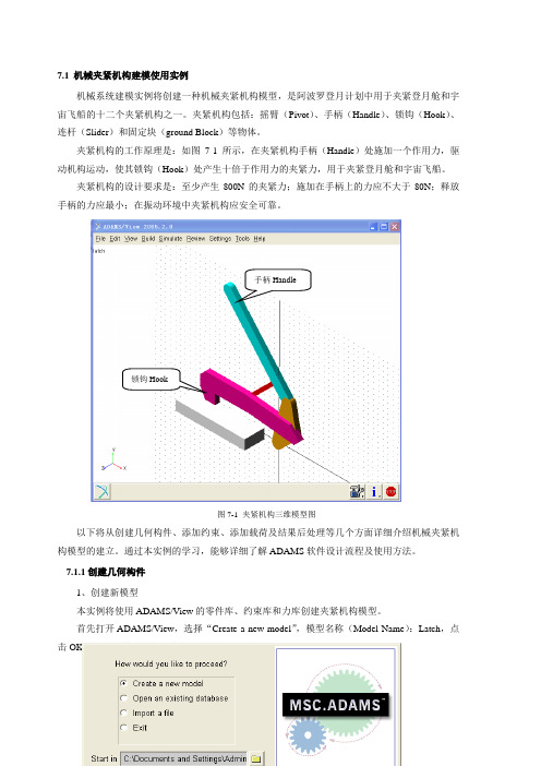
7.1机械夹紧机构建模使用实例机械系统建模实例将创建一种机械夹紧机构模型,是阿波罗登月计划中用于夹紧登月舱和宇宙飞船的十二个夹紧机构之一。
夹紧机构包括:摇臂(Pivot)、手柄(Handle)、锁钩(Hook)、连杆(Slider)和固定块(ground Block)等物体。
夹紧机构的工作原理是:如图7-1所示,在夹紧机构手柄(Handle)处施加一个作用力,驱动机构运动,使其锁钩(Hook)处产生十倍于作用力的夹紧力,用于夹紧登月舱和宇宙飞船。
夹紧机构的设计要求是:至少产生800N的夹紧力;施加在手柄上的力应不大于80N;释放手柄的力应最小;在振动环境中夹紧机构应安全可靠。
手柄Handle锁钩Hook图7-1 夹紧机构三维模型图以下将从创建几何构件、添加约束、添加载荷及结果后处理等几个方面详细介绍机械夹紧机构模型的建立。
通过本实例的学习,能够详细了解ADAMS软件设计流程及使用方法。
7.1.1创建几何构件1、创建新模型本实例将使用ADAMS/View的零件库、约束库和力库创建夹紧机构模型。
首先打开ADAMS/View,选择“Create a new model”,模型名称(Model Name):Latch,点击OK,创建新模型完毕。
其它设置如图7-2所示:图7-2 创建新模型2、设置工作环境选择菜单栏【Settings】→【Units】命令,设置模型物理量单位,如图7-3所示:图7-3设置模型物理量单位选择菜单栏【Settings】→【Working Grid】命令,设置工作网格,如图7-4所示:图7-4设置工作网格3、创建设计点设计点是几何构件形状设计和位置定位的参考点。
本实例将通过设计点列表编辑器创建几何构件模型所需要的全部设计点。
选择并点击几何模型库(Geometric Modeling)中的点(Point),下拉菜单选择(Add to Ground)、(Don’t Attach),并单击Point Table列表编辑器,创建并生成Point_1、Point_2等六个设计点,如图7-5、图7-6所示:图7-5设计点列表编辑器图7-6创建设计点4、创建摇臂(Pivot)选择并点击几何模型库(Geometric Modeling)中的平板(Plate),设置平板厚度值(Thickness)为1,圆角半径(Radius)为1,用鼠标左键选择设计点:Point_1、Point_2、Point_3,按鼠标右键完成摇臂(Pivot)的创建,将其重新命名(Rename)为Pivot,如图7-7所示:图7-7创建摇臂5、创建手柄(Handle)选择并点击几何模型库(Geometric Modeling)中的连杆(Link),用鼠标左键选择设计点:Point_3和Point_4,完成手柄(Handle)的创建,将其重新命名(Rename)为Handle,如图7-8所示:图7-8创建手柄6、创建锁钩(Hook)选择并点击几何模型库(Geometric Modeling)中的拉伸体(Extrusion),选择“New Part”和“Clsoed”,拉伸体长度(Lengh)设为1,用鼠标左键选择表7-1所示的11个位置,按鼠标右键完成锁钩的创建,将其重新命名(Rename)为Hook,如图7-9示:表7-1锁钩节点坐标X坐标Y坐标Z坐标1 5 3 02 3 5 03 -6 6 04 -14 6 05 -15 5 06 -15 3 07 -14 1 08 -12 1 09 -12 3 010 -5 3 011 4 2 0图7-9创建锁钩7、创建连杆(Slider)选择并点击几何模型库(Geometric Modeling)中的连杆(Link),用鼠标左键选择设计点:Point_5和Point_6,完成连杆(Slider)的创建,将其重新命名(Rename)为Slider,如图7-10所示:图7-10创建连杆8、创建固定块(Ground Block)选择并点击几何模型库(Geometric Modeling)中的长方体(Box),选择“On Ground”,使其与大地(Ground)固结在一起,按下图创建固定体用鼠标左键选择设计点:Point_5和Point_6,完成连杆(Slider)的创建,将其重新命名(Rename)为Slider,如图7-11所示:图7-11创建固定块7.1.2添加约束1、添加旋转约束副选择并点击约束库(Joints)中的旋转副(Revolute Joints);选择“1 Location”(一个位置),“Normal To Grid”(垂直于工作网络),用鼠标左键选择Point_1,创建摇臂和大地的约束副;选择“2 Bodies - 1 Location”(两个物体一个位置),“Normal To Grid”(垂直于工作网络),选择摇臂和锁钩两个物体,左键选择Point_2,创建摇臂和锁钩的约束副;同理选择摇臂和手柄,位置为Point_3,手柄和连杆,位置为Point_5,创建摇臂和手柄、手柄和连杆的旋转约束副。
基于LQR控制的现代客车自适应空气悬架

10.16638/ki.1671-7988.2021.06.031基于LQR控制的现代客车自适应空气悬架王旭(扬州亚星客车股份有限公司,江苏扬州225116)摘要:长期在不良工况的道路上驾驶会降低驾驶员的乘坐舒适性。
随着人们对乘坐舒适性需求不断提升,空气弹簧的优势尤为明显。
文章提出了一种基于LQR控制策略的自适应空气悬架系统的创新设计方案,提出的LQR控制器采用粒子群算法进行优化。
以客车空气悬架为研究对象,采用MATLAB软件对空气悬架系统的被动和自适应动力学模型进行了设计和仿真。
仿真结果表明,自适应空气悬架系统在保证车辆稳定性的同时,降低了车辆在随机道路上的最大位移幅值,从而提高了车辆的平顺性。
关键词:空气悬架;PID;PSO;自适应悬架;乘坐舒适性中图分类号:U461.4 文献标识码:A 文章编号:1671-7988(2021)06-101-04Modern passenger car adaptive air suspension based on LQR controlWang Xu( Yangzhou Yaxing Bus Co., Ltd., Jiangsu Yangzhou 225116 )Abstract: Driving on the road under bad working conditions for a long time will reduce the driver's riding comfort. With the increasing demand for ride comfort, the advantage of air spring is especially obvious. This paper presents an innovative design scheme of adaptive air suspension system based on LQR control strategy. The proposed LQR controller is optimized by particle swarm optimization. The passive and adaptive dynamic models of the air suspension system of passenger cars were designed and simulated by MATLAB software. The simulation results show that the adaptive air suspension system can not only ensure the stability of the vehicle, but also reduce the maximum displacement amplitude of the vehicle on the random road, thus improving the ride comfort of the vehicle.Keywords: Air suspension; PID; PSO; Adaptive suspension; Ride comfortCLC NO.: U461.4 Document Code: A Article ID: 1671-7988(2021)06-101-041 引言对驾驶舒适性需求的增加要求在汽车上使用主动悬架系统。
MATLAB软件在汽车悬架系统的模拟与分析中的应用
摘要汽车悬架系统是整个汽车中非常重要的一个环节,它性能的好坏直接影响到汽车的平顺性和安全性,而主动悬架系统能使汽车的乘坐舒适性以及操纵稳定性和安全性得到很大程度的提高,因此,主动悬架系统是现代汽车的一个发展方向。
本文分别对汽车的被动悬架系统和主动悬架系统建立了双轴四自由度的模型,列出了这两种模型的状态方程,并结合现代控制理论中的线性调节器理论对主动悬架的控制原理进行了分析。
本人在分析悬架系统工作特性的基础上使用了c 语言对MATLAB软件进行了二次开发,开发出的这套软件它能对不同型号的被动悬架系统和主动悬架系统汽车进行模拟仿真,并进行分析,因此命名为SAS软件(以下简称SAS)。
利用SAS软件对被、主动悬架进行了模拟分析,根据模拟的结果对被动悬架和主动悬架汽车的性能进行了对比分析,并对其平顺性进行了评价。
关键词:悬架、主动、被动、MATLAB模拟ABSTACTSuspension system is one of the most important part in the whole automobiles. Its performance influences directly on ride comfort and safety of auto. Active-suspension is able to improve greatly the performances of auto such as ride comfort, security and stability. Hence developing and designing the active-suspension is the important direction in the future.In the paper ,I set up two four-freedom models about passive suspension and active-suspension of vehicles, and list their state space equations. Moreover, I analyze the controlling principle of active-suspension by using the modern controlling theory.I develop a set of software based on the MATLAB software by using C language according to suspension performance. Its main functions are to simulate the passive-suspension and active suspension about vehicles whose construction parameters are variable and then analyze the suspension. So I call this software SAS software (short for SAS). Using SAS software, I simulate the passive-suspension and active-suspension. According to the result after simulating, I analyze and compare performances of two kinds of suspensions, and furthermore evaluate the ride comfort on vehicles.Keywords: suspension active passive MATLAB simulation第二章建立汽车悬架系统的状态方程2. 2汽车被动悬架系统状态方程的建立根据上一节的分析,我们可以把汽车被动悬架系统简化为一个如图2所示的1/2车辆模型。
- 1、下载文档前请自行甄别文档内容的完整性,平台不提供额外的编辑、内容补充、找答案等附加服务。
- 2、"仅部分预览"的文档,不可在线预览部分如存在完整性等问题,可反馈申请退款(可完整预览的文档不适用该条件!)。
- 3、如文档侵犯您的权益,请联系客服反馈,我们会尽快为您处理(人工客服工作时间:9:00-18:30)。
Modeling for Bus Suspension System:The Code.function bus_modclear allclcm1 = 2800;m2 = 350;k1 = 80000;k2 = 500000;b1 = 350;b2 = 15020;nump=[(m1+m2) b2 k2]; % defining the order of the numerator for actuated force input.denp=[(m1*m2) (m1*(b1+b2))+(m2*b1) (m1*(k1+k2))+(m2*k1)+(b1*b2) (b1*k2)+(b2*k1) k1*k2]; %defining the denomenator for acutated force input.'G(s)1' % standard transfer function G1.printsys(nump,denp)%PRINTSYS is used to print state space systems with labels to the%right and above the system matrices or to print transfer functions%as a ratio of two polynomials.num1=[-(m1*b2) -(m1*k2) 0 0]; %defining numerator for disturbance input.den1=[(m1*m2) (m1*(b1+b2))+(m2*b1) (m1*(k1+k2))+(m2*k1)+(b1*b2) (b1*k2)+(b2*k1) k1*k2]; %defining the denomenator for disturbance input.'G(s)2'printsys(0.1*num1,den1)%%%%%%OPEN LOOP RESPONSE%%%%%%figure (1)step(nump,denp);%from the graph it is clear that for a unit step actuated force the%response of the system is underdamped. People sittig in the bus will feel%very small amount of oscillation and steady-state error is about 0.013mm.%Moreover, the bus takes very unacceptably long time for it to reach the%steady state or the settling time is very large. The solution to this%problem is to add a feedback controller into the system's block diagram.figure (2)step(0.1*num1,den1);axis([0 10 -.1 .1]); %details for the response.%From this graph of open-loop response for 0.1 m step disturbance, we can%see that when the bus passes a 10 cm high bump on the road, the bus body%will oscillate for an unacceptably long time(100 seconds) with larger amplitude,%13 cm, than the initial impact. People sitting in the bus will not be comfortable%with such an oscillation. The big overshoot (from the impact itself) and the slow%settling time will cause damage to the suspension system. The solution to this%problem is to add a feedback controller into the system to improve the performance.Results.G(s)1num/den =3150 s^2 + 15020 s + 500000-----------------------------------------------------------------------980000 s^4 + 43158500 s^3 + 1657257000 s^2 + 1376600000 s + 40000000000 G(s)2num/den =-4205600 s^3 - 140000000 s^2-----------------------------------------------------------------------980000 s^4 + 43158500 s^3 + 1657257000 s^2 + 1376600000 s + 40000000000 Plots.PID Controller for Bus Suspension System:The Code.function bus_pidclear allclcm1 = 2800;m2 = 350;k1 = 80000;k2 = 500000;b1 = 350;b2 = 15020;nump=[(m1+m2) b2 k2]; % defining the order of the numerator for actuated force input.denp=[(m1*m2) (m1*(b1+b2))+(m2*b1) (m1*(k1+k2))+(m2*k1)+(b1*b2) (b1*k2)+(b2*k1) k1*k2]; %defining the denomenator for acutated force input.num1=[-(m1*b2) -(m1*k2) 0 0]; %defining numerator for disturbance input.den1=[(m1*m2) (m1*(b1+b2))+(m2*b1) (m1*(k1+k2))+(m2*k1)+(b1*b2) (b1*k2)+(b2*k1) k1*k2]; %defining the denomenator for disturbance input.%%%%Adding Feedback%%%numf = num1;denf = nump;%%%Adding PID%%%%KD = 2*2.08e6;KP = 2*8.32e6;KI = 2*6.24e6;numc = [KD,KP,KI]; %equation for numerator.denc = [1 0]; % single s in the denominatornuma = conv(numf,denc);dena = polyadd(conv(denp,denc),conv(nump,numc));%%%Closed Loop Response%%%t = 0:0.05:5;figure (1)step(0.1*numa,dena,t)title('closed-loop response to 0.1m high step with pid controller')z1 = 1; %first zero at originz2 = 3; %second zero at a distance from first one.p1 = 0; %pole at zero.numc = conv([1 z1],[1 z2]) %convolution of numerator zerosdenc = [1 p1] % equation of pole, independent S.num2 = conv(nump,numc);den2 = conv(denp,denc);figure (2)rlocus(num2,den2)title('root locus with PID controller')[K,p]=rlocfind(num2,den2)The Results.numc = 1 4 3denc = 1 0Select a point in the graphics window selected_point = -11.1611 + 6.3354i K =3.2575e+004p = 1.0e+002 *The Plots.Root Locus for Bus Suspension System.The Code.function bus_rlclear allclcm1 = 2800;m2 = 350;k1 = 80000;k2 = 500000;b1 = 350;b2 = 15020;nump=[(m1+m2) b2 k2]; % defining the order of the numerator for actuated force input.denp=[(m1*m2) (m1*(b1+b2))+(m2*b1) (m1*(k1+k2))+(m2*k1)+(b1*b2) (b1*k2)+(b2*k1) k1*k2]; %defining the denomenator for acutated force input.num1=[-(m1*b2) -(m1*k2) 0 0]; %defining numerator for disturbance input.den1=[(m1*m2) (m1*(b1+b2))+(m2*b1) (m1*(k1+k2))+(m2*k1)+(b1*b2) (b1*k2)+(b2*k1) k1*k2]; %defining the denomenator for disturbance input.%%%%Adding Feedback%%%numf = num1;denf = nump;R = roots(denp) %open loop poles%%%plotting the root locus%%%%figure (1)rlocus(nump,denp) %plotting of ROOT LOCUS.axis([-40 40 -60 60])z = -log(0.05)/sqrt(pi^2+(log(0.05)^2))sgrid(z,0)%%%Adding a Notch filter%%%%z1 = 3 + 3.5i;z2 = 3 - 3.5i;p1 = 30;p2 = 60;numc = conv([1 z1],[1 z2]);denc = conv([1 p1],[1 p2]);figure (2)rlocus(conv(nump,numc),conv(denp,denc))axis([-40 10 -30 30])z = -log(0.05)/sqrt(pi^2+(log(0.05)^2))sgrid(z,0)title('Root Locus with Notch Filter')%%%gain from the root locus%%%[k,poles] = rlocfind(conv(nump,numc),conv(denp,denc))numc = k*numc;numa = conv(conv(numf,nump),denc);dena = conv(denf,polyadd(conv(denp,denc),conv(nump,numc)));%%%%Plotting the closed-loop response%%%figure(3)step(0.1*numa,dena)The Results.R =-21.9215 +34.3118i-21.9215 -34.3118i-0.0981 + 4.9609i-0.0981 - 4.9609iz =0.6901Select a point in the graphics window selected_point = -10.4384 + 2.8882i k = 3.4667e+006poles =1.0e+002 *The Plots.Frequency Response for Bus Suspension.The Code.function bus_frclear allclcm1 = 2800;m2 = 350;k1 = 80000;k2 = 500000;b1 = 350;b2 = 15020;nump=[(m1+m2) b2 k2]; % defining the order of the numerator for actuated force input.denp=[(m1*m2) (m1*(b1+b2))+(m2*b1) (m1*(k1+k2))+(m2*k1)+(b1*b2) (b1*k2)+(b2*k1) k1*k2]; %defining the denomenator for acutated force input.num1=[-(m1*b2) -(m1*k2) 0 0]; %defining numerator for disturbance input.den1=[(m1*m2) (m1*(b1+b2))+(m2*b1) (m1*(k1+k2))+(m2*k1)+(b1*b2) (b1*k2)+(b2*k1) k1*k2]; %defining the denomenator for disturbance input.%%%%Adding Feedback%%%numf = num1;denf = nump;%%%%Plotting the Frequency Response by BODE%%%figure(1)nump=100000*nump;w = logspace(-1,2);bode(nump,denp,w)%%%Adding a Two Lead Controller%%%%%%figure(2)numc=conv([1.13426 1], [1.13426 1]);denc=conv([0.035265 1], [0.035265 1]);margin(conv(nump,numc),conv(denp,denc))w=logspace(-4,4);figure(3)[mag,phase,w] = bode(conv(nump,numc),conv(denp,denc),w);subplot(2,1,1);semilogx(w,20*log10(mag));grid ontitle('Bode plot of system with notch filter')xlabel('Frequency (rad/s)')ylabel('20logM')subplot(2,1,2);semilogx(w,phase);axis([1e-4, 1e4, -180, 360])grid onxlabel('Frequency (rad/s)')ylabel('Phase (degrees)')State Space Design for Bus Suspension.The Code.function bus_ssclear allclcm1 = 2800; m2 = 350; k1 = 80000; k2 = 500000; b1 = 350; b2 = 15020;A=[0 1 0 0-(b1*b2)/(m1*m2) 0 ((b1/m1)*((b1/m1)+(b1/m2)+(b2/m2)))-(k1/m1) -(b1/m1) b2/m2 0 -((b1/m1)+(b1/m2)+(b2/m2)) 1k2/m2 0 -((k1/m1)+(k1/m2)+(k2/m2)) 0];B=[0 01/m1 (b1*b2)/(m1*m2)0 -(b2/m2)(1/m1)+(1/m2) -(k2/m2)];C=[0 0 1 0];D=[0 0];%%%%%%%%Designing a State feedback controller%%%%%%Aa = [[A,[0 0 0 0]'];[C, 0]];Ba = [B;[0 0]];Ca = [C,0];Da = D;K = [0 2.3e6 5e8 0 8e6]figure(1)t=0:0.01:2;step(Aa-Ba(:,1)*K,-0.1*Ba,Ca,Da,2,t)title('Closed-loop response to a 0.1 m step')Result. K = 0 2300000 500000000 0 8000000。