Isokinetic Dynamometry in Anterior Cruciate Ligament Injury and Reconstruction

合集下载

Kinetic Monte Carlo simulations of heteroepitaxial growth with an atomistic model

Kinetic Monte Carlo simulations of heteroepitaxial growth with an atomistic model of elasticityPinku Nath,Madhav Ranganathan ⁎Department of Chemistry,Indian Institute of Technology Kanpur,Kanpur 208016,Indiaa b s t r a c ta r t i c l e i n f o Article history:Received 7February 2012Accepted 21May 2012Available online 28May 2012Keywords:Heteroepitaxial systemsKinetic Monte Carlo simulations Submonolayer growth Atomic elasticityWe have implemented Kinetic Monte Carlo (KMC)simulations of growth of heteroepitaxial thin ﬁlms.A sim-ple cubic Solid-on-Solid (SOS)model is used to describe the atomic con ﬁgurations and nearest neighbor bonds are used to describe the energetics.Elastic effects are modeled using harmonic springs between atoms displaced from their lattice positions.The mis ﬁt strain is a consequence of different equilibrium spring lengths for the substrate and ﬁlm.The consistency of this elastic model with continuum theories for strained surfaces has been shown by performing elastic energy calculations for various morphologies.KMC simula-tions for submonolayer deposition show scaling behavior in the island size distribution.The resulting island shapes are predominantly square and do not show any shape transitions in the physically relevant range of conditions.This method gives a detailed understanding of elastic interactions and their interplay with surface diffusion in heteroepitaxial systems.©2012Elsevier B.V.All rights reserved.1.IntroductionStrained heteroepitaxial systems like Germanium (Ge)on Silicon (Si)are characterized by a small mismatch between the lattice parameters of the two materials,the ﬁlm and the substrate.This mis ﬁt can affect the morphology of these ﬁlms.For example,it is well known that a growing heteroepitaxial ﬁlm develops spontaneous undulations that eventually lead to formation of mounds and,sometimes,quantum dots [1–3].Controlled growth processes like Molecular Beam Epitaxy (MBE)can be used to closely study these phenomena and also grow high quality ﬁlms and nanostructures [4–15].Heteroepitaxial systems have been of interest for nanoscale optoelectronic devices [16–18];e.g.Field-Effect-Transistors made with Si/Ge [19],GaAsP/InGaAs quantum wells for solar cells [20].The nature of growth of a strained ﬁlm is in ﬂuenced by the mis ﬁt.For Ge on Si(100),the mis ﬁt is about 4%.The ﬁrst few layers of the ﬁlm grow ﬂat over the substrate.As more layers are deposited,the strain accumulated in the ﬁlm increases and this causes spontaneous mound formation in the ﬁlm (Fig.2).This type of growth is called Stranski –Krastanov growth [1,21]and is also found in other heteroepitaxial systems like InAs/GaAs [22].The transition from layer-by-layer growth to mound formation after a certain number of layers is referred to as the 2D/3D growth transition.For systems with larger mis ﬁt,it is expected that this transition will be observed at lower coverages.It has been reported that the wetting layer in Ge/Si(100)is about 4–5ML thick [23]where it is about 1–2ML thick forInAs/GaAs [24].The shapes and size distribution of the mounds have also been a subject of many experimental [2,25,7]and theoretical stud-ies [26–31].The behavior during the early stages of mound formation,when the coverage is less than 1ML,has been investigated experimentally [32–34]and theoretically [35–42].During this stage the surface is mostly covered with monolayer islands of different sizes.The shape and size distribution of these islands depend on the surface studied.For example,in the case of Ge/Si(100),these islands are mostly rectan-gular in shape.The relative role of mis ﬁt strain and anisotropic surface energy in the shape and size of these islands is a question of interest to us.KMC simulations have proved to be very useful for the study of surface morphology during growth [43].KMC allows us to study the interplay between deposition and surface diffusion during growth of a certain surface.For heteroepitaxial systems,the elastic strain modi ﬁes the surface diffusion rates.These elastic effects are inherently long range effects.Due to this reason,the resulting KMC scheme is no longer a local scheme.Strain effects have been included in KMC simulations in many different ways.One class of approaches involves calculation of the elastic response of the semi-in ﬁnite substrate medium to the forces caused by the morphological features on the surface,like steps,adatoms,etc.The elastic response is typically calculated using continuum approaches involving Green's functions [41,44–46].Alternatively,the effect of elastic strain can be modeled using a reduction in the diffusion barrier for atoms in the ﬁlm [37],or as an effective interaction between surface atoms in the ﬁlm [40].In this article we focus on KMC simula-tions in which elastic effects are included through an atomistic model of elasticity with harmonic springs [47–50].Our method is closelySurface Science 606(2012)1450–1457⁎Corresponding author.Tel.:+915122596037;fax:+915122597436.E-mail address:madhavr@iitk.ac.in (M.Ranganathan).0039-6028/$–see front matter ©2012Elsevier B.V.All rights reserved.doi:10.1016/j.susc.2012.05.015Contents lists available at SciVerse ScienceDirectSurface Sciencej o u r na l h o me p a g e :ww w.e l s e v i e r.c o m /l o c a t e /s u s crelated to a prior work in this area,and we apply the method of calcu-lations on a realistic system.The elastic energy calculation involves a multidimensional minimization of the total energy of all the harmonic springs in the system.This makes the elastic computation extremely time-consuming.To implement this model in a KMC simulation,it is therefore necessary to come up with a set of approximations that will reduce the number of elasticity calculations.The rest of this article is organized as follows:In Section 2,we de-scribe the multicomponent Solid-on-Solid model that we use to de-scribe the surface.In Section 3,we show the KMC simulation method and the calculation of the surface hopping probabilities.In Section 4,we explain the model of elasticity used for the heteroepitaxial system.In Section 5,we illustrate how the KMC simulations can be performed with explicit elastic effects.In Section 6,we describe some results of our work,ﬁrst on elastic energy calculations,and then submonolayer growth simulations.Finally,we make summarize the key ﬁndings and give our outlook on future work in this area in Section 7.2.Multicomponent Solid-on-Solid modelWe present here a lattice model for studying the evolution of the surface of a multicomponent system.Our model is based on the sim-ple cubic Solid-on-Solid (SOS)model,in which the crystal lattice is described by a 2D array of columns of various heights [51,43].For the single component SOS model,it is suf ﬁcient to specify the heights of the columns in order to specify the surface.In the multicomponent case,each lattice site can be occupied by one of the various species as shown in Fig.1.In general,the behavior of the surface is dependent on the nature of the species in the columns.Hence it is essential in this model to have a variable to describe the type of the atom in each of the occupied lattice sites.Further,we impose a no-overhang condition,according to which a lattice site can only be occupied if the site one layer below is also occupied.The multicomponent SOS model can then be implemented in a Kinetic Monte Carlo (KMC)scheme in way similar to the standard SOS model using moves to describe the various processes of interest.The crystal is assumed to be growing in the +Z (upward)direction.The substrate is considered to in ﬁnitely thick and extend all the way to Z =−∞.We impose periodic boundary conditions in the X and Ydirections with the supercell dimension to be a multiple of the substrate lattice constant a s .Our simulations are designed to model the Ge on Si(100).We note that the systems we are considering do not have a simple cubic lattice,and the true Si(100)surface is reconstructed.The focus of this article is to study the interplay between elasticity and sur-face diffusion and we expect that the qualitative features of this behavior will be reproduced reasonably well in the simple cubic model.In the rest of this article,we will be using “Si ”and “Ge ”to refer to the substrate and ﬁlm respectively.3.Kinetic Monte Carlo methodWe consider the dynamical processes taking place on the crystal surface during a typical MBE experiment,namely deposition and surface diffusion.We neglect bulk diffusion,defect formation and migration,and exchange of atoms in the bulk of the crystal.Surface diffusion is modeled by thermally activated hopping of surface atoms at random to their neighboring sites.The rate of this process can be written down in the Arrhenius form as r ¼ν0exp −E b =k B T ðÞð1Þwhere E b is energy barrier that has to be overcome in order for the atom to hop,k B is the Boltzmann constant,T is the absolute temperature and ν0is the attempt frequency.The attempt frequency ν0is independent of temperature and its value is around 1013s −1,corresponding to vibra-tional frequency of an atom in the lattice site.We assume the same value of ν0for all surface atoms in the system.The hopping rates satisfy the detailed balance condition,so thatr i →j ðÞ¼e −E j =k B T e −E i =k B ¼P eqj ðÞeq ð2Þwhere r (i →j )is the rate of transition from con ﬁguration i to j involving a surface atom,and E i and E j are the energies of the two con ﬁgurations and P eq (i )and P eq (j )are their respective equilibriumprobabilities.Fig.1.Typical con ﬁguration in a two-component simple cubic SOS model (left)and a cross-sectional view of the rectangular section (right).The black and white balls represent different atoms.For example,the black atoms can be Si atoms and the white atoms can beGe.Fig.2.A cartoon showing how strain caused by mismatch between the ﬁlm (gray circles)and the substrate (black circles)is signi ﬁcantly relaxed at surfaces,and at the edges of steps andmounds.Fig.3.The elastic model showing springs between NN and NNN atoms for a typical con-ﬁguration.The springs in the ﬁlm (gray)have different parameters than in the substrate (black).In a typical optimization to calculate the elastic energy,we consider numerically op-timize displacements in the top few layers of the substrate (two layers in the above ﬁgure),and solve for the displacement ﬁeld analytically in the rest of the semi-in ﬁnite substrate;as indicated by the wavy lines.1451P.Nath,M.Ranganathan /Surface Science 606(2012)1450–1457Detailed balance ensures that when there is no deposition,the system will tend towards equilibrium with a Boltzmann distribution of energy.In the simulation of this model,we carry out a combination of random deposi-tion and hopping moves with the appropriate acceptance rates.The barrier energy E b is the total energy that a surface atom needs to have in order to hop to a neighboring site.In the absence of elastic energy,this barrier is the energy required to break all the bonds of the atom.The value of this barrier depends on the number and strength of these bonds,so E b =E bond =∑j γj where γi is the strength of the bond between the atom (which we attempt to hop)and the i th atom.The sum is performed over all the bonds of the surface atom.The strength of the bond depends on the particular model of interac-tion chosen.For example,if we are describing a Ge atom on the (100)surface of Si using our simple cubic lattice,we use a nearest neighbor (NN)interaction model consisting of two kinds of bonds with energies E h and E v corresponding to bonds in the horizontal and vertical direc-tions respectively.In the absence of elastic energy,the barrier energy is a local quantity which can be stored for all surface atoms.After every move,the barrier energy of a small number of atoms has to be updated.This makes it possible to implement the KMC using a rejection-free method similar to the Bortz –Kalos –Lebowitz algorithm [52].This is not possible when we include elastic effects.Hence,we implement a KMC scheme with ac-ceptance and rejection of atom hopping moves so as to satisfy Eq.(1).4.Elastic modelThe lattice mismatch of a heteroepitaxial ﬁlm is de ﬁned as =(a f −a s )/a s where a f and a s represent the lattice constants of ﬁlm and the substrate respectively.For a ﬁlm of Ge on Si,this value is around 4%.This mismatch can be controlled by depositing a mixture of Si and Ge on the ﬁlm of varying concentrations.Following previous work [53,54],we implement a model of hetero-epitaxy using springs between atoms.This model is explained in the references but we give a brief review here.Associated with each atom is a 3-dimensional elastic displacement from its lattice position.Each atom is connected by springs to its nearest neighbors (NN)and next nearest neighbors (NNN)(Fig.3).The energy of each spring is given by E spring =(1/2)k (d −l eq )2where d is the distance between the atoms and l eq is the equilibrium length at which the spring energy is zero and k is the spring constant.The distance d between atoms on neigh-boring lattice sites is calculated geometrically using the lattice constants and the elastic displacements.The values of k and l eq depend on the nature of the bond (NN or NNN),and the species of atoms forming the bond.For a pure cubic system,the two independent elastic moduli,C 11and C 12,are related to the spring constants by the relations [55]k L ¼a C 11−2C 12ðÞk D ¼aC 12ð3Þwhere k L and k D are the spring constants for the NN and NNN bonds re-spectively,and a is the equilibrium length of the lateral springs in the simple cubic lattice model.The elastic energy leads to a restoring force in the system that tries to minimize the spring energy of each atom.In order to model heteroepitaxial systems,we assign different equilibrium spring lengths to the ﬁlm and the substrate atoms corresponding to their lattice con-stants.The equilibrium bond lengths of the NN and the NNN bonds in the ﬁlm are a f and a f ﬃﬃﬃ2p .We assumed that the spring constants k L and k D remain the same for different kinds of atoms,and that the equilibrium length of a bond between the substrate atom and the ﬁlm atom is equal to that of a bond between two ﬁlm atoms.We will discuss the implica-tions of these assumptions later.The cell periodicity ensures that for a pure substrate,there are no elas-tic effects.When a single complete monolayer is deposited on the sub-strate,the bonds are compressed in the horizontal (X and Y)directionsas shown in Fig.3.This causes the ﬁlm to expand in the Z-direction.The equilibrium location of the atoms in the Z direction can be calculated using the minimum energy or zero force condition.Under this condition,the separation of atoms in the Z-direction,a L can be obtained by solving k L a L −a s ðÞþ4k D ðﬃﬃﬃﬃﬃﬃﬃﬃﬃﬃﬃﬃﬃﬃﬃﬃa 2Lþa 2s q −a f ﬃﬃﬃ2p Þa L ﬃﬃﬃﬃﬃﬃﬃﬃﬃﬃﬃﬃﬃﬃﬃﬃa 2L þa 2sq ¼0:ð4ÞThe elastic energy is a function of the displacements of all the atoms.By minimizing this function with respect to the displacements,we cal-culate the optimum displacements.This is the elastic relaxation that has to be carried out at every step of the Kinetic Monte Carlo simulation.We can do this using any of the standard multidimensional minimization routines like conjugate gradient,steepest descent,etc.We are interested in growth of a thin ﬁlm on a large substrate.For a semi-in ﬁnite substrate with given displacements of the topmost layer,the elastic displacements of the substrate are calculated analytically based on the procedure outlined in Ref.[47].In this procedure,we line-arize the springs in the substrate and expand the displacement vector ﬁeld {U }in a Fourier basis in the X and Y directions.This Fourier trans-form,~U n o decays exponentially inside the substrate.We expand ~U n o using eigenvalues and eigenvectors and the coef ﬁcients are calculatedusing the displacements of the topmost layer of the substrate.The dis-placement ﬁeld {U }is used to calculate the contribution to the elastic energy from the substrate.This procedure allows us to greatly reduce the number of atoms involved in the elastic energy calculation.In practice,we treat a few layers of the substrate as discrete layers before treating the remaining as a continuum as shown in Fig.3.Since we treat a few layers of the substrate as discrete layers,we can potentially model intermixing wherein atoms from the substrate migrate into the ﬁlm.This intermixing is believed to be one of the mechanisms for strain relaxation in these systems.We end this section with a few comments about the elastic model and the KMC simulations.Firstly,our KMC simulations are implemented on a Simple cubic SOS model.We allow for atoms to hop from one site to one of their neighboring sites.The elastic displacements are localized on the lattice sites.These displacements are used in the calculation of the distance between two atoms on neighboring lattice sites.It is,therefore,implicit that these displacements are not too large (not greater than half the spacing between atoms).Secondly,there are some parameters in the model like the spring constants and the equilibrium lengths for all the different types of bonds.The equilibrium lengths of bonds involving only one kind of atom are based on the bulk lattice constants of the atom.But there is some arbitrariness in the choice of the equilibrium length for a bond involving two different atoms.The spring constants of bonds involving only the ﬁlm or the substrate atoms are chosen so as to reproduce the bulk elastic moduli for these systems.ThereisFig.4.The interaction energy between the ridge and trench features of the inset for D =4plotted as a function of d .The dots show the results of our model and the solid curve is f (d )of Eq.(5)multiplied by 2.2.1452P.Nath,M.Ranganathan /Surface Science 606(2012)1450–1457again some arbitrariness in the choice of the spring constant for a bond involving two different atoms.In particular,the choices of these param-eters inﬂuence the wetting layer and the2D/3D growth transition.Fur-ther,real Si or Ge is neither cubic,nor isotropic.In fact the diffusion of Ge atoms on Si(100)surface has been shown to be strongly anisotropic because of the2×1reconstruction.Due to the above reasons,we feel that our model can be used to study the qualitative behavior,but care should be exercised while making quantitative comparisons to other models and experiments.Finally,we note that for an individual atom, the elastic energy is typically a very small part of the entire barrier energy in the KMC simulations discussed in the next section.Despite this,it is be-lieved to play an important role in the structures formed during growth.5.KMC simulations with elasticityThe KMC method we have described in Section3is implemented using the hopping rate given by Eq.(1).The barrier energy is treated as a sum of the energy due to the bonds and the elastic energy due to the displacements.The displacements are calculated for aﬁxed conﬁg-uration of atoms.Implicit in this method is the assumption that the elas-tic relaxation of the system takes place on much timescale smaller than that of surface diffusion.The elastic energy causes a reduction of the barrier for surface diffusion,since the springs in our model cannot have energies less than zero.Thus we can write E b=E bond−E el,where E el is the elastic energy contribution to the hopping barrier.To calculate E el,we need to calculate the difference of the total elastic energy of the system with and without the atom.Each elastic energy calculation needs a minimization of the energy function to calculate the atomic dis-placements.The elastic energy computation is the most expensive part of the entire calculation.We therefore consider some approximate schemes that will minimize the number of these calculations.Firstly we assume that the dominant contribution to the elastic en-ergy comes from the elastic springs of the atom to its NN and NNN atoms.Thus we approximate E el as E el¼∑bonds12k bond l bond−l eq bondÀÁ2 where k bond is the spring constant of the bond,l bond is the distance be-tween the atoms forming the bond,and l bondeq is the equilibrium bond length.This approximation allows us to calculate the elastic energy of the atom from its conﬁguration without having to consider the elastic energy of the system without the atom.This reduces the total number of elastic energy calculations by a factor of2.In order to construct more approximations,we need to use some information about the elastic energy.Let us consider an adatom,i.e.a surface atom that is only bonded to one NN and4NNN atoms.Since the bond energy is only due to NN atoms,the total bond energy of an adatom is equal to E v.For an arbitrary surface,the elastic energy of an adatom depends on the detailed conﬁguration of the surface.If the surface is notﬂat, the energy of adatoms located at different points on the surface will be different.As we shall show in Section1,this difference in elastic energy of adatoms on a given layer is negligible compared to the elastic energy of other surface atoms.We neglect this difference in our KMC simulations.This greatly simpliﬁes the elastic energy calculation for adatoms.The elastic energy plays an important role in the diffusion of other surface atoms and has to be calculated accurately for those atoms.Since a signiﬁcant fraction of atomic moves on the surface in-volve adatoms,our approximation leads to a signiﬁcant time-saving. Further,since there are very few atoms that have fewer bonds than adatoms,we will set the time unit in our KMC simulations as the time for one adatom hop.With this approximation,we can write the hopping rate r as r=r ad exp−(E b−E b ad/k B T)where r ad is the hopping rate of an adatom and E b ad is the total barrier energy for an adatom.We choose our timestep so that r ad=1,thereby eliminating rejection of moves in-volving adatoms.This makes it possible to extend our simulations to longer times and study the growth of multiple layers.A similar approx-imation has been used recently in Ref.[50].We mention one more detail about the adatom energies here.The energy of aﬁlm adatom on aﬂat substrate depends on the bond energy and the elastic interaction parameters involving theﬁlm and the sub-strate atoms.As we had mentioned earlier,there is someﬂexibility as regards the various parameters for a bond involving two different atoms.If we assume that the elastic parameters and the bonds are iden-tical for the interface layer and theﬁlm,then weﬁnd that adatoms from different layers hop at the same rate.Any other choice will lead to an adatom hopping frequency that is dependent on the number of layers. Such dependence plays a role in the transition from2D layer-by-layer growth to3D mound growth.For instance,slower diffusion of adatoms in the upper layers will favor3D growth.A layer dependent adatom energy(elastic or bond)corresponds to a wetting layer in our system.A more careful examination of the wetting layer and the2D/3D transition will be the subject of a subsequent article.6.Results and discussionWe divide our results into two sections.In theﬁrst,we discuss elasticity calculations for various conﬁgurations.These calculations validate the model,and help us in constructing the approximations that were discussed in Section5.In the second,we discuss KMC sim-ulations of submonolayer growth.All calculations were carried out on a128×128system.The various parameters were chosen to mimic the Ge on Si(100).The lattice spacing in Si is2.715Åand that in Ge is 2.832Å.We performed Fourier transforms using the Fast Fourier Transform routine[56].The eigenvalues and eigenvectors for the substrate contribution were calculated using the singular value de-composition routine in LAPACK[57].The multidimensional minimi-zation of the elastic energy to calculate the elastic displacements was accomplished using the conjugate gradient optimizer in the GNU Scientiﬁc Library[58].The spring constants are taken as k L=73eV/nm2and k D=96eV/nm2to approximately reproduce the elastic moduli of Si.We have used the same spring constants for all pairs of atoms.The equilibrium bond length of a bond involving an Si and a Ge atom was taken to be equal to that of a Ge bond.To compare the submonolayer growth calculations with earlier work,we have used a temperature of500K,E v=0.8eV and E h=0.3eV.We have used the same value of E v for Ge atoms on bare Si(100)and Ge atoms atop Ge islands.The surface diffusion coefﬁcient D s can be estimated as D s=(1/4)ν0exp(−E v/k B T)a s2which works out to about2×104s−1in length units of a s.Since we ignored all the anisotropic effects in the hop-ping barriers,we do not have any anisotropy in the surface diffusion constant.Besides the Si–Ge model system(4%misﬁt),we have per-formed calculations for systems with no misﬁt and8%misﬁt.Though we do not show this result here,we have veriﬁed that3D island forma-tion was observed at low coverages(b0.5ML)when we used8%misﬁt and spring constants larger by a factor of10.Each KMC simulation tra-jectory was generated on a64-bit Intel X5500series processor;and120 parallel trajectories were simulated to get good statistics.A simulation of1ML on these systems took about144h;but the simulation time in-creases for subsequent layers because of the increase in the total num-ber ofﬁlm atoms.6.1.Elastic energy calculationsIt has been proposed that the elastic interaction energy between two adatoms a distance r apart on aﬂat epitaxial layer is proportional to1/r3. This interaction is due to force dipoles located near each of the adatoms. On the other hand,steps on strainedﬁlms cause force monopoles and the interaction between steps distance r apart is proportional to log(r).For a periodic array of steps,the dependence is slightly modiﬁed.We test this dependence by performing elastic calculations for the conﬁguration shown with d and D in Fig.4.We calculated the elastic energies of a ﬂat surface E f,a surface with a ridge E r,a surface with a trench E t and a surface with both a ridge and a trench E rt.The elastic energy1453P.Nath,M.Ranganathan/Surface Science606(2012)1450–1457of interaction between the ridge and the trench features U int is given by U int =E rt −E r −E t +E f .According to continuum elasticity theory,this interaction energy is proportional tof d ðÞ¼−logsin 2πd þD ðÞ=L ðÞ"#ð5Þwhere L is the periodicity of the system.The constant of proportionality is related to the magnitude of the force monopoles at the step edges.We show that our interaction energy can be ﬁtted to Eq.(5)with a single ﬁtting parameter.The difference at smaller distances is simply a consequence of the difference between the continuum model and our lattice model at short length scales.In general,we expect to see some differences for moder-ate length scales,so it is remarkable that the graph in Fig.4agrees so well at moderate length scales.It is possibly due to the symmetric na-ture of the con ﬁgurations considered.Analogous to the usual thermodynamic chemical potential,we de ﬁne an elastic chemical potential μel of an adatom on a given surface as the dif-ference in the elastic energy of the system with and without the adatom.For a given con ﬁguration of a surface,μel changes for different locations asshown in Fig.5.The ﬁgure illustrates that the elastic contribution to the hopping barrier is largest at the island edges and is almost constant along a ﬂat surface.Thus the atoms at the edges of islands have a reduced hopping barrier due to elasticity.The adatoms on top of the island have a smaller elastic energy than those on the bare substrate.The reduction in elastic energy causes slower diffusion of adatoms on top of islands.These two effects eventually lead to a transition from layer-by-layer growth to 3D mound formation in the KMC simulations.As a ﬁnal demonstration of our elastic model,we show the dependence of μel at the island edges on the size of the island in Fig.6.The increase in island energy with island size follows a trend consistent with the continuum elasticity based calcu-lations of Refs.[41,37].As the size of the islands becomes large,the elastic energy increases much more slowly.We note that the chemical potential as calculated by us is signi ﬁcantly smaller than that calculated in Ref.[41].This difference will be re ﬂected again in the results of the KMC simula-tions in the next section.6.2.Submonolayer growthWhen Ge atoms are deposited on an atomically ﬂat Si substrate,the deposited atoms diffuse on the surface and,occasionally,get attached to Ge islands on the surface.The resulting surface shows many islands typ-ically of different sizes as shown in Fig.7for different values of the mis-match.In Fig.7(d),we show a snapshot of a system with 4%mismatch,but a spring constant 5times larger.In this case,we can see some mul-tilayer islands too.If the deposition rate is slow,then the adatoms have suf ﬁcient time to get attached to existing islands and the average size of islands is large.The island size distribution therefore depends on the ratio of the surface diffusion coef ﬁcient to the ﬂux,i.e.the D s /F ratio.We performed KMC simulations of submonolayer growth of Ge on Si.By choosing F =0.1ML/s and F =10ML/s,we get D s /F ratios of 2×105and 2×103(in units of a s 2)respectively.Following the previous section,we take a constant elastic energy for adatoms on any given layer.KMC simulations of submonolayer growth have been performed earlier using continuum elasticity model [41]and using an effective adatom interaction model [40].In both these cases the island size distribution for a given D s /F ratio was consistent with the scaling form [40,38]N s θðÞb s >2θ¼f s =b s >ðÞð6Þwhere N s represent number of islands of size s (s ≥2)when the surface coverage is θand the average island size is b s >.This form was derived for irreversible submonolayer growth conditions in the absence of elas-tic interactions.In Fig.8,we show the scaled island size distribution as a function of s /b s >for θ=0.1−0.29for F =0.1ML/s.The points seem to ﬁt on a master curve indicating that there is very little mound formation.Chemical potential (meV)b)a)102030Elastic Displacementsc)Fig.5.(a)Graph showing μel of an adatom located at various distances on the surface along the line AB.The inset ﬁgure shows part of the surface con ﬁguration with the line AB.(b)A contour map of μel on a surface with a 9×9island,and (c)cross-section of the surface showing the elastic displacement of atoms (magni ﬁed by factor 10for better visibility)in the vicinity of an island.102030400200400600µe l (m e V )sFig.6.μel for a Ge adatom next to a square Ge island of size s .1454P.Nath,M.Ranganathan /Surface Science 606(2012)1450–1457。

英语翻译

金属聚氨酯，聚氨酯-脲和聚氨酯-醚综述摘要由于聚氨酯具有优良的耐磨性，弹性和塑性，它在工程材料中变得越来越重要。

随着聚氨酯科学与技术的发展，促进了具有更多的令人满意的性能的新材料的发展。

这种材料包括含金属的聚氨酯类，聚氨酯-脲和聚氨酯-醚，它们有异氰酸酯的结构单元，并且增强了热稳定性，阻燃性，柔软性和溶解性。

合成含金属的聚氨酯最初的原料用含金属离子的二醇盐，此时金属牢固的融入了聚合物的主链中。

把金属引入聚氨酯中使得其具有广泛的应用，比如在水性增稠剂、浸渍剂、纺织施胶剂、粘合剂、添加剂、树脂和催化剂上的应用。

本文主要介绍了制备包含金属的聚氨酯各种合成方法，以及其共聚物性能。

1.引言聚氨酯代表了热塑性和热固性的一类重要聚合物，是因为通过不同的多元醇与多异氰酸酯反应调整其机械性能、热的和化学性能。

聚氨酯含有大量的氨基甲酸酯（-HN-COO-），不论其他部分是什么。

通常，通过多异氰酸酯与含有至少两个羟基的反应物如聚醚、蓖麻油和简单的二醇，两者组合来获得PU。

其他活性基像氨基和羧基也可能存在。

因此，这种典型的聚氨酯除了含有氨基甲酸酯基团外，还有酯、醚、酰胺和脲基。

从二醇（HO-R-OH）和二异氰酸酯（OCN-R’-NCO）的结构可以得出线性聚氨酯的一般结构如下：PU的性能根据其需求在许多方面都不同。

羟基化合物和异氰酸酯基的功能基增加到三个或者更多，以此来形成支链或者交联聚合物。

还可以通过R（聚醚、聚酯和乙二醇）的性质做其他结构的改变，也可以通过改变R'的分子量和类型改变R'。

由于这些原因，PU的交联性和链柔软性和其分子间力可以广泛而且独立的变化。

一般来讲，由于P中U通过聚多元醇的软链段和氨基甲酸酯的极性官能团增强的弹性性能，使PU呈现出良好的粘合性能。

这些材料被广泛的应用于涂料、泡沫材料、和不同的塑料和弹性体。

金属聚氨酯代表了把无机盐连接到聚合物链上的一个广泛聚合物的分类。

一般，当他们有充足的离子电荷在水中溶解时，我们把它称为“聚合物电解质”，如果含有离子基的浓度太低以至于不能水解时，我们称之为“离子聚合物”。

专业英语

Definition of polymers A simple understanding of polymers can be gained by imaging them to be like a chain or, perhaps, a string of pearls, where the individual pearl represent small molecules that are chemically bonded together. Therefore, a polymer is a molecule made up of smaller molecules that are joined together by chemical bonds. The word polymer means „many parts or units.‟ The parts or units are the small molecules that combine. The result of the combination is, of course, a chainlike molecule (polymer). Usually the polymer chains are long, often consisting of hundreds of units, but polymers consisting of only a few units linked together are also known and can be commercially valuable.
Figure 1.1 Diagram illustrating the definition of plastics.
As Figure 1.1 shows, all materials can be classified as gases, simple liquids, or solids, with the understanding that most materials can be converted from one state to another through heating or cooling. If only materials that are structural solids at normal temperatures are examined, three major types of materials are encountered: metals, polymers, and ceramics. The polymer materials can be further divided into synthetic polymers and natural polymers. Most synthetic polymers are those that do not occur naturally and are represented by materials such as nylon, polyethylene, and polyester. Some synthetic polymers could be manufactured copies of naturally occurring materials (such as

英文翻译

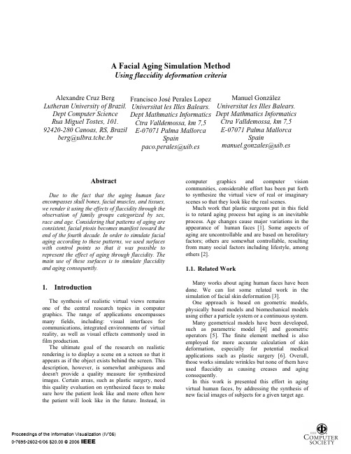
A Facial Aging Simulation Method Using flaccidity deformation criteriaAlexandre Cruz Berg Lutheran University of Brazil.Dept Computer ScienceRua Miguel Tostes, 101. 92420-280 Canoas, RS, Brazil berg@ulbra.tche.br Francisco José Perales LopezUniversitat les Illes Balears.Dept Mathmatics InformaticsCtra Valldemossa, km 7,5E-07071 Palma MallorcaSpainpaco.perales@uib.esManuel GonzálezUniversitat les Illes Balears.Dept Mathmatics InformaticsCtra Valldemossa, km 7,5E-07071 Palma MallorcaSpainmanuel.gonzales@uib.esAbstractDue to the fact that the aging human face encompasses skull bones, facial muscles, and tissues, we render it using the effects of flaccidity through the observation of family groups categorized by sex, race and age. Considering that patterns of aging are consistent, facial ptosis becomes manifest toward the end of the fourth decade. In order to simulate facial aging according to these patterns, we used surfaces with control points so that it was possible to represent the effect of aging through flaccidity. The main use of these surfaces is to simulate flaccidity and aging consequently.1.IntroductionThe synthesis of realistic virtual views remains one of the central research topics in computer graphics. The range of applications encompasses many fields, including: visual interfaces for communications, integrated environments of virtual reality, as well as visual effects commonly used in film production.The ultimate goal of the research on realistic rendering is to display a scene on a screen so that it appears as if the object exists behind the screen. This description, however, is somewhat ambiguous and doesn't provide a quality measure for synthesized images. Certain areas, such as plastic surgery, need this quality evaluation on synthesized faces to make sure how the patient look like and more often how the patient will look like in the future. Instead, in computer graphics and computer vision communities, considerable effort has been put forthto synthesize the virtual view of real or imaginary scenes so that they look like the real scenes.Much work that plastic surgeons put in this fieldis to retard aging process but aging is an inevitable process. Age changes cause major variations in the appearance of human faces [1]. Some aspects of aging are uncontrollable and are based on hereditary factors; others are somewhat controllable, resulting from many social factors including lifestyle, among others [2].1.1.Related WorkMany works about aging human faces have been done. We can list some related work in the simulation of facial skin deformation [3].One approach is based on geometric models, physically based models and biomechanical models using either a particle system or a continuous system.Many geometrical models have been developed, such as parametric model [4] and geometric operators [5]. The finite element method is also employed for more accurate calculation of skin deformation, especially for potential medical applications such as plastic surgery [6]. Overall, those works simulate wrinkles but none of them have used flaccidity as causing creases and aging consequently.In this work is presented this effort in aging virtual human faces, by addressing the synthesis of new facial images of subjects for a given target age.We present a scheme that uses aging function to perform this synthesis thru flaccidity. This scheme enforces perceptually realistic images by preserving the identity of the subject. The main difference between our model and the previous ones is that we simulate increase of fat and muscular mass diminish causing flaccidity as one responsible element for the sprouting of lines and aging human face.In the next section will plan to present the methodology. Also in section 3, we introduce the measurements procedure, defining structural alterations of the face. In section 4, we present a visual facial model. We describe age simulation thrua deformation approach in section 5. In the last section we conclude the main results and future work.2.MethodologyA methodology to model the aging of human face allows us to recover the face aging process. This methodology consists of: 1) defining the variations of certain face regions, where the aging process is perceptible; 2) measuring the variations of those regions for a period of time in a group of people and finally 3) making up a model through the measurements based on personal features.That could be used as a standard to a whole group in order to design aging curves to the facial regions defined.¦njjjpVM2.1Mathematical Background and AnalysisHuman society values beauty and youth. It is well known that the aging process is influenced by several parameters such: feeding, weight, stress level, race, religious factors, genetics, etc. Finding a standard set of characteristics that could possibly emulate and represent the aging process is a difficult proposition.This standard set was obtained through a mathematical analysis of some face measurements in a specific group of people, whose photographs in different ages were available [7]. To each person in the group, there were, at least, four digitized photographs. The oldest of them was taken as a standard to the most recent one. Hence, some face alterations were attained through the passing of time for the same person.The diversity of the generated data has led to the designing of a mathematical model, which enabled the acquiring of a behavior pattern to all persons of the same group, as the form of a curve defined over the domain [0,1] in general, in order to define over any interval [0,Į] for an individual face. The unknown points Įi are found using the blossoming principle [8] to form the control polygon of that face.The first step consisted in the selection of the group to be studied. Proposing the assessment of the face aging characteristics it will be necessary to have a photographic follow-up along time for a group of people, in which their face alterations were measurable.The database used in this work consisted of files of patients who were submitted to plastic surgery at Medical Center Praia do Guaíba, located in Porto Alegre, Brazil.3.MeasurementsAccording to anatomic principles [9] the vectors of aging can be described aswhich alter the position and appearance of key anatomic structures of the face as can be shown in figure 1 which compares a Caucasian mother age 66 (left side) with her Caucasian daughters, ages 37 (right above) and 33 (right below) respectively.Figure 1 - Observation of family groupsTherefore, basic anatomic and surgical principles must be applied when planning rejuvenative facial surgery and treating specific problems concomitantwith the aging process.4.Visual Facial ModelThe fact that human face has an especially irregular format and interior components (bones, muscles and fabrics) to possess a complex structure and deformations of different face characteristics of person to person, becomes the modeling of the face a difficult task. The modeling carried through in the present work was based on the model, where the mesh of polygons corresponds to an elastic mesh, simulating the dermis of the face. The deformations in this mesh, necessary to simulate the aging curves, are obtained through the displacement of the vertexes, considering x(t) as a planar curve, which is located within the (u,v ) unit square. So, we can cover the square with a regular grid of points b i,j =[i/m,j/n]T ; i=0,...,m; j=0,...,n. leading to every point (u,v ) asfrom the linear precision property of Bernstein polynomials. Using comparisons with parents we can distort the grid of b i,j into a grid b'i,j , the point (u,v )will be mapped to a point (u',v') asIn order to construct our 3D mesh we introduce the patch byAs the displacements of the vertexes conform to the certain measures gotten through curves of aging and no type of movement in the face is carried through, the parameters of this modeling had been based on the conformation parameter.4.1Textures mappingIn most cases the result gotten in the modeling of the face becomes a little artificial. Using textures mapping can solve this problem. This technique allows an extraordinary increase in the realism of the shaped images and consists of applying on the shaped object, existing textures of the real images of the object.In this case, to do the mapping of an extracted texture of a real image, it is necessary that the textureaccurately correspond to the model 3D of that is made use [9].The detected feature points are used for automatic texture mapping. The main idea of texture mapping is that we get an image by combining two orthogonal pictures in a proper way and then give correct texture coordinates of every point on a head.To give a proper coordinate on a combined image for every point on a head, we first project an individualized 3D head onto three planes, the front (x, y), the left (y, z) and the right (y, z) planes. With the information of feature lines, which are used for image merging, we decide on which plane a 3D-head point on is projected.The projected points on one of three planes arethen transferred to one of feature points spaces suchas the front and the side in 2D. Then they are transferred to the image space and finally to the combined image space.The result of the texture mapping (figure 2) is excellent when it is desired to simulate some alteration of the face that does not involve a type of expression, as neutral. The picture pose must be the same that the 3D scanned data.¦¦¦ mi nj lk n j m i lk k j i w B v B u B b w v u 000,,)()()(')',','(¦¦ m i nj n jmij i v B u B b v u 00,)()(),(¦¦ m i nj n j m i j i v B u B b v u 00,)()(')','(¦¦¦ mi nj lk n j m i lk k j i w B v B u B b w v u 000,,)()()(')',','(Figure 2 - Image shaped with texturemapping5.Age SimulationThis method involves the deformation of a face starting with control segments that define the edges of the faces, as¦¦¦ mi nj lk n j m i lk k j i w B v B u B b w v u 000,,)()()(')',','(Those segments are defined in the original face and their positions are changed to a target face. From those new positions the new position of each vertex in the face is determined.The definition of edges in the face is a fundamental step, since in that phase the applied aging curves are selected. Hence, the face is divided in influencing regions according to their principal edges and characteristics.Considering the face morphology and the modeling of the face aging developed [10], the face was divided in six basic regions (figure 3).The frontal region (1) is limited by the eyelids and the forehead control lines. The distance between these limits enlarges with forward aging.The orbitary region (2) is one of the most important aging parameters because a great number of wrinkles appears and the palpebral pouch increases [11]. In nasal region (3) is observed an enlargement of its contour.The orolabial region (4) is defined by 2 horizontal control segments bounding the upper and lower lips and other 2 segments that define the nasogenian fold. Figure 3 - Regions considering the agingparametersThe lips become thinner and the nasogenian fold deeper and larger. The mental region (5) have 8 control segments that define the low limit of the face and descend with aging. In ear curve (6) is observed an enlargement of its size. The choice of feature lines was based in the characteristic age points in figure 6.The target face is obtained from the aging curves applied to the source face, i.e., with the new control segment position, each vertex of the new image has its position defined by the corresponding vertex in the target face. This final face corresponds to the face in the new age, which was obtained through the application of the numerical modeling of the frontal face aging.The definition of the straight-line segment will control the aging process, leading to a series of tests until the visual result was adequate to the results obtained from the aging curves. The extremes of the segments are interpolated according to the previously defined curves, obtained by piecewise bilinear interpolation [12].Horizontal and vertical orienting auxiliary lines were defined to characterize the extreme points of the control segments (figure 4). Some points, that delimit the control segments, are marked from the intersection of the auxiliary lines with the contour of the face, eyebrow, superior part of the head and the eyes. Others are directly defined without the use of auxiliary lines, such as: eyelid hollow, eyebrow edges, subnasion, mouth, nasolabial wrinkle andnose sides.Figure 4 - Points of the control segmentsOnce the control segments characterize the target image, the following step of the aging process can be undertaken, corresponding to the transformations of the original points to the new positions in the target image. The transformations applied to the segments are given by the aging curves, presented in section 4.In the present work the target segments are calculated by polynomial interpolations, based on parametric curves [12].5.1Deformation approachThe common goal of deformation models is to regulate deformations of a geometric model by providing smoothness constraints. In our age simulation approach, a mesh-independent deformation model is proposed. First, connected piece-wise 3D parametric volumes are generated automatically from a given face mesh according to facial feature points.These volumes cover most regions of a face that can be deformed. Then, by moving the control pointsof each volume, face mesh is deformed. By using non-parallel volumes [13], irregular 3D manifolds are formed. As a result, smaller number of deformvolumes are necessary and the number of freedom incontrol points are reduced. Moreover, based on facialfeature points, this model is mesh independent,which means that it can be easily adopted to deformany face model.After this mesh is constructed, for each vertex on the mesh, it needs to be determined which particularparametric volume it belongs to and what valueparameters are. Then, moving control points ofparametric volumes in 3D will cause smooth facialdeformations, generating facial aging throughflaccidity, automatically through the use of the agingparameters. This deformation is written in matricesas , where V is the nodal displacements offace mesh, B is the mapping matrix composed ofBernstein polynomials, and E is the displacementvector of parametric volume control nodes.BE V Given a quadrilateral mesh of points m i,j ,, we define acontinuous aged surface via a parametricinterpolation of the discretely sampled similaritiespoints. The aged position is defined via abicubic polynomial interpolation of the form with d m,n chosen to satisfy the known normal and continuity conditions at the sample points x i,j .>@>M N j i ,...,1,...,1),(u @@>@>1,,1,),,( j j v i i u v u x ¦3,,),(n m n m n m v u d v u x An interactive tool is programmed to manipulate control points E to achieve aged expressions making possible to simulate aging through age ranges. Basic aged expression units are orbicularis oculi, cheek, eyebrow, eyelid, region of chin, and neck [14]. In general, for each segment, there is an associated transformation, whose behavior can be observed by curves. The only segments that do not suffer any transformation are the contour of the eyes and the superior side of the head.5.2Deformation approachThe developed program also performs shape transformations according to the created aging curves, not including any quantification over the alterations made in texture and skin and hair color. Firstly, in the input model the subjects are required to perform different ages, as previouslymentioned, the first frame needs to be approximately frontal view and with no expression.Secondly, in the facial model initialization, from the first frame, facial features points are extracted manually. The 3D fitting algorithm [15] is then applied to warp the generic model for the person whose face is used. The warping process and from facial feature points and their norms, parametric volumes are automatically generated.Finally, aging field works to relieve the drifting problem in template matching algorithm, templates from the previous frame and templates from the initial frame are applied in order to combine the aging sequence. Our experiments show that this approach is very effective. Despite interest has been put in presenting a friendly user interface, we have to keep in mind that the software system is research oriented. In this kind of applications an important point is the flexibility to add and remove test facilities. 6.Results The presented results in the following figuresrefer to the emulations made on the frontalphotographs, principal focus of this paper, with theobjective to apply the developed program to otherpersons outside the analyzed group. The comparisonswith other photographs of the tested persons dependon their quality and on the position in which theywere taken. An assessment was made of the new positions, of the control segments. It consisted in: after aging a face, from the first age to the second one, through the use of polynomial interpolation of the control segments in the models in the young age, the new positions are then compared with the ones in the model of a relative of older age (figure 5). The processed faces were qualitatively compared with theperson’s photograph at the same age. Figure 5 - Synthetic young age model,region-marked model and aged modelAlso the eyelid hollow, very subtle falling of the eyebrow, thinning of the lips with the enlarging of the nasion and the superior part of the lip, enlargingof the front and changing in the nasolabial wrinkle.7.ConclusionsModelling biological phenomena is a great deal of work, especially when the biggest part of the information about the subject involves only qualitative data. Thus, this research developed had has a challenge in the designing of a model to represent the face aging from qualitative data.Due to its multi-disciplinary character, the developed methodology to model and emulate the face aging involved the study of several other related fields, such as medicine, computing, statistics and mathematics.The possibilities opened by the presented method and some further research on this field can lead to new proposals of enhancing the current techniques of plastic face surgery. It is possible to suggest the ideal age to perform face lifting. Once the most affected aging regions are known and how this process occurs over time. Also missing persons can be recognized based on old photographs using this technique. AcknowledgementsThe project TIN2004-07926 of Spanish Government have subsidized this work.8. References[1] Burt, D. M. et al., Perc. age in adult Caucasianmale faces, in Proc. R. Soc., 259, pp 137-143,1995.[2] Berg, A C. Aging of Orbicularis Muscle inVirtual Human Faces. IEEE 7th InternationalConference on Information Visualization, London, UK, 2003a.[3] Beier , T., S. Neely, Feature-based imagemetamorphosis, In Computer Graphics (Proc.SIGGRAPH), pp. 35-42, 1992.[4] Parke, F. I. P arametrized Models for FacialAnimation, IEEE Computer & Graphics Applications, Nov. 1982.[5] Waters, K.; A Muscle Model for Animating ThreeDimensional Facial Expression. Proc SIGGRAPH'87,Computer Graphics, Vol. 21, Nº4, United States, 1987. [6] Koch, R.M. et alia.. Simulation Facial SurgeryUsing Finite Element Models, Proceedings of SIGGRAPH'96, Computer Graphics, 1996.[7] Kurihara, Tsuneya; Kiyoshi Arai, ATransformation Method for Modeling and Animation of the Human Face from Photographs, Computer Animatio n, Springer-Verlag Tokyo, pp.45-58, 1991.[8] Kent, J., W. Carlson , R. Parent, ShapeTransformation for Polygon Objects, In Computer Graphics (Proc. SIGGRAPH), pp. 47-54, 1992. [9] Sorensen, P., Morphing Magic, in ComputerGraphics World, January 1992.[10]Pitanguy, I., Quintaes, G. de A., Cavalcanti, M.A., Leite, L. A. de S., Anatomia doEnvelhecimento da Face, in Revista Brasileira deCirurgia, Vol 67, 1977.[11]Pitanguy, I., F. R. Leta, D. Pamplona, H. I.Weber, Defining and measuring ageing parameters, in Applied Mathematics and Computation , 1996.[12]Fisher, J.; Lowther, J.; Ching-Kuang S. Curveand Surface Interpolation and Approximation: Knowledge Unit and Software Tool. ITiCSE’04,Leeds, UK June 28–30, 2004.[13]Lerios, A. et al., Feature-Based VolumeMetamorphosis, in SIGGRAPH 95 - Proceedings,pp 449-456, ACM Press, N.Y, 1995.[14]Berg, A C. Facial Aging in a VirtualEnvironment. Memória de Investigación, UIB, Spain, 2003b.[15]Hall, V., Morphing in 2-D and 3-D, in Dr.Dobb's Journal, July 1993.。

纳米管制作皮肤感应器翻译中英

最后译文：纳米管弹性制作出皮肤般的感应器美国斯坦福大学的研究者发现了一种富有弹性且透明的导电性能非常好的薄膜，这种薄膜由极易感触的碳纳米管组成，可被作为电极材料用在轻微触压和拉伸方面的传感器上。

“这种装置也许有一天可以被用在被截肢者、受伤的士兵、烧伤方面接触和压迫的敏感性的恢复上，也可以被应用于机器人和触屏电脑方面”，这个小组如是说。

鲍哲南和他的同事们在他们的弹透薄膜的顶部和底部喷上一种碳纳米管的溶液形成平坦的硅板，覆盖之后，研究人员拉伸这个胶片，当胶片被放松后，纳米管很自然地形成波浪般的结构，这种结构作为电极可以精准的检测出作用在这个材料上的力量总数。

事实上，这种装配行为上很像一个电容器，用硅树脂层来存储电荷，像一个电池一样，当压力被作用到这个感应器上的时候，硅树脂层就收紧，并且不会改变它所储存的电荷总量。

这个电荷是被位于顶部和底部的硅树脂上的纳米碳管测量到的。

当这个复合膜被再次拉伸的时候，纳米管会自动理顺被拉伸的方向。

薄膜的导电性不会改变只要材料没有超出最初的拉伸量。

事实上，这种薄膜可以被拉伸到它原始长度的2.5倍，并且无论哪种方向不会使它受到损害的拉伸它都会重新回到原始的尺寸，甚至在多次被拉伸之后。

当被充分的拉伸后，它的导电性喂2200S/cm，能检测50KPA的压力，类似于一个“坚定的手指捏”的力度，研究者说。

“我们所制作的这个纳米管很可能是首次可被拉伸的，透明的，肤质般感应的，有或者没有碳的纳米管”小组成员之一Darren Lipomi.说。

这种薄膜也可在很多领域得到应用，包括移动设备的屏幕可以感应到一定范围的压力而不仅限于触摸；可拉伸和折叠的几乎不会毁坏的触屏感应器；太阳能电池的透明电极；可包裹而不会起皱的车辆或建筑物的曲面；机器人感应装置和人工智能系统。

其他应用程序“其他系统也可以从中受益—例如那种需要生物反馈的—举个例子，智能方向盘可以感应到，如果司机睡着了，”Lipomi补充说。

新滋养保养新概念

Strengthens Communication Connection
润肤/防护润肤防护 MOISTURISE/PREVENT 滋养日间防护乳霜/液滋养日间防护乳霜液 SPF15/PA+++
TIME DEFIANCE Day Protect Crème/Lotion SPF 15/PA+++
Youthful Skin with Derma Cell Exchange
表皮和真皮间结合层
表皮层
真皮层
日间
晚间
活化 STIMULATE 活肤脂类基质 HLM+:
• 重新平衡养分与脂质。Rebalances Moisture and Lipid Levels 重新平衡养分与脂质。 • 促进皮肤内部脂质的生成。Encourages Lipid Production from Within 促进皮肤内部脂质的生成。 • 重新启动细胞间的信息交流。Restarts the Communication Process 重新启动细胞间的信息交流。
西柚GRAPEFRUIT
保护PROTECT 保护防晒保护 SPF 15/PA+++:
• 为皮肤提供对抗紫外线的侵害为皮肤提供对抗紫外线的侵害。
Skin’s Best Defense Against UV Damage
帮助抑制自由基。 • 帮助抑制自由基
Protects & Neutralizes Free Radical Damage
抗氧化复合成分 4.0 主要成分
Defense Complex 4: Ingredients
第一阶段：第一阶段：超氧化物歧化酶
STAGE 1: Superoxide Dismutase

【高考生物】王玉梅托福词汇里的生物类单词总结

（生物科技行业）王玉梅托福词汇里的生物类单词总结adaptadapableadaptation--modification(以上三词都与动物进化有关) antibiotic抗菌的，抗生的antibiotics抗生素aquaticadj.水生的，水栖的aquariumn.水族馆arborealadj.树栖的，树的；乔木的arid--dryadj.干旱的semiaridadj.雨量特别少的aroman. 芳香，香气aromatic--fragrantadj.芳香的fragrant--aromatica,fragrance--scentn,香味perfumen,香味，香水backbone--spinen,脊椎，中枢baldeagle秃头鹰（美国国鸟）bardn, 鱼钩等的 - 倒勾，倒刺；bark--outercoveringn,树皮n/vi. 狗叫beakn, 鸟嘴polarbear北极熊grizzlybear灰熊biologistn.生物学家biologicaldiversity生物多样性bisonn. 美洲或欧洲的野牛bloomn/vi. 花/ 开花blossomn/vi. 花/ 开花boardern,寄生者baboonn,狒狒bouquetn,花簇breed--raise,hatch,matevt,养育，生殖n,品种crossbreedingn,异种杂交budn, 芽，蓓蕾vi, 萌芽bulbn ，球茎cannibalismn,同类相食carapacen,龟蟹等得-甲壳cardiacadj,心脏的，cardinaladj, 红衣凤头鸟 - 一种美洲鸟，雄性有深红色羽毛carnivorousadj,食肉的caterpillarn,毛虫chimpanzeen,黑猩猩gorillan,大猩猩calmn, 蚌肉clutchn, 一次所孵的蛋condorn,秃鹰conifern,松类针叶树coralreef珊瑚礁carbn, 蟹crawl--creepvi,爬行crown, 乌鸦crustaceann，甲壳动物culturevi,培养（微生物细胞组织等）daisyn, 雏菊deciduousadj,每年落叶的，decompositionn,腐化，分解decompose--decayv,分解，使腐化rodentn,edentaten,贫齿类动物dolphinn,海豚domesticate-cultivatevt,驯养驯化domesticated-tameadj. dormantadj,休眠的endotoxinn,内梅素endothermn,恒温动物draftanimal耕种动物（ horse之类）dragonflyn,蜻蜓ecologicaladj,生态学的，生态的ecologistnecologynecologistemn生态系统embryo-completelyundevelopedformn,胚胎；embryologicaladj,胚胎学的embryonicadj,萌芽期的，endanger-threaen,jeopardizevt,危及endangeredadj,有灭绝危险的，将要绝种的evergreenadj 常绿的， n,常绿植物extinctadj, 动物 -灭绝的；extinctionn.falconn, 猎鹰falconern,养猎鹰之人faunan, 动物群floran植物群floraladj,花的，植物的feedv, 饲养，靠。

南开大学光学工程专业英语重点词汇汇总

光学专业英语部分refraction [rɪˈfrækʃn]n.衍射reflection [rɪˈflekʃn]n.反射monolayer['mɒnəleɪə]n.单层adj.单层的ellipsoid[ɪ'lɪpsɒɪd]n.椭圆体anisotropic[,ænaɪsə(ʊ)'trɒpɪk]adj.非均质的opaque[ə(ʊ)'peɪk]adj.不透明的；不传热的；迟钝的asymmetric[,æsɪ'metrɪk]adj.不对称的；非对称的intrinsic[ɪn'trɪnsɪk]adj.本质的，固有的homogeneous[,hɒmə(ʊ)'dʒiːnɪəs;-'dʒen-] adj.均匀的；齐次的；同种的；同类的，同质的incidentlight入射光permittivity[,pɜːmɪ'tɪvɪtɪ]n.电容率symmetric[sɪ'metrɪk]adj.对称的；匀称的emergentlight出射光；应急灯.ultrafast[,ʌltrə'fɑ:st,-'fæst]adj.超快的；超速的uniaxial[,juːnɪ'æksɪəl]adj.单轴的paraxial[pə'ræksɪəl]adj.旁轴的；近轴的periodicity[,pɪərɪə'dɪsɪtɪ]n.[数]周期性；频率；定期性soliton['sɔlitɔn]n.孤子，光孤子；孤立子；孤波discrete[dɪ'skriːt]adj.离散的，不连续的convolution[,kɒnvə'luːʃ(ə)n]n.卷积；回旋；盘旋；卷绕spontaneously:[spɒn'teɪnɪəslɪ] adv.自发地；自然地；不由自主地instantaneously:[,instən'teinjəsli]adv.即刻；突如其来地dielectricconstant[ˌdaiiˈlektrikˈkɔnstənt]介电常数，电容率chromatic[krə'mætɪk]adj.彩色的；色品的；易染色的aperture['æpətʃə;-tj(ʊ)ə]n.孔，穴；（照相机，望远镜等的）光圈，孔径；缝隙birefringence[,baɪrɪ'frɪndʒəns]n.[光]双折射radiant['reɪdɪənt]adj.辐射的；容光焕发的；光芒四射的; photomultiplier[,fəʊtəʊ'mʌltɪplaɪə]n.[电子]光电倍增管prism['prɪz(ə)m]n.棱镜；[晶体][数]棱柱theorem['θɪərəm]n.[数]定理；原理convex['kɒnveks]n.凸面体；凸状concave['kɒnkeɪv]n.凹面spin[spɪn]n.旋转；crystal['krɪst(ə)l]n.结晶，晶体；biconical[bai'kɔnik,bai'kɔnikəl] adj.双锥形的illumination[ɪ,ljuːmɪ'neɪʃən] n.照明；[光]照度；approximate[ə'prɒksɪmət] adj.[数]近似的；大概的clockwise['klɒkwaɪz]adj.顺时针方向的exponent[ɪk'spəʊnənt；ek-] n.[数]指数；even['iːv(ə)n]adj.[数]偶数的；平坦的；相等的eigenmoden.固有模式；eigenvalue['aɪgən,væljuː]n.[数]特征值cavity['kævɪtɪ]n.腔；洞，凹处groove[gruːv]n.[建]凹槽，槽；最佳状态；惯例；reciprocal[rɪ'sɪprək(ə)l]adj.互惠的；相互的；倒数的，彼此相反的essential[ɪ'senʃ(ə)l]adj.基本的；必要的；本质的；精华的isotropic[,aɪsə'trɑpɪk]adj,各向同性的；等方性的phonon['fəʊnɒn]n.[声]声子cone[kəʊn]n.圆锥体，圆锥形counter['kaʊntə]n.柜台；对立面；计数器；cutoff['kʌt,ɔːf]n.切掉；中断；捷径adj.截止的；中断的cladding['klædɪŋ]n.包层；interference[ɪntə'fɪər(ə)ns]n.干扰，冲突；干涉borderline['bɔːdəlaɪn]n.边界线，边界；界线quartz[kwɔːts]n.石英droplet['drɒplɪt]n.小滴，微滴precision[prɪ'sɪʒ(ə)n]n.精度，[数]精密度；精确inherently[ɪnˈhɪərəntlɪ]adv.内在地；固有地；holographic[,hɒlə'ɡræfɪk]adj.全息的；magnitude['mægnɪtjuːd]n.大小；量级；reciprocal[rɪ'sɪprək(ə)l]adj.互惠的；相互的；倒数的，彼此相反的stimulated['stimjə,letid]v.刺激（stimulate的过去式和过去分词）cylindrical[sɪ'lɪndrɪkəl]adj.圆柱形的；圆柱体的coordinates[kəu'ɔ:dineits]n.[数]坐标；external[ɪk'stɜːn(ə)l;ek-]n.外部；外观；scalar['skeɪlə]n.[数]标量；discretization[dɪs'kriːtaɪ'zeɪʃən]n.[数]离散化synthesize['sɪnθəsaɪz]vt.合成；综合isotropy[aɪ'sɑtrəpi]n.[物]各向同性；[物]无向性；[矿业]均质性pixel['pɪks(ə)l;-sel]n.（显示器或电视机图象的）像素（passive['pæsɪv]adj.被动的spiral['spaɪr(ə)l]n.螺旋；旋涡；equivalent[ɪ'kwɪv(ə)l(ə)nt]adj.等价的，相等的；同意义的; transverse[trænz'vɜːs;trɑːnz-;-ns-]adj.横向的；横断的；贯轴的;dielectric[,daɪɪ'lektrɪk]adj.非传导性的；诱电性的;n.电介质；绝缘体integral[ˈɪntɪɡrəl]adj.积分的；完整的criteria[kraɪ'tɪərɪə]n.标准，条件（criterion的复数）Dispersion:分散|光的色散spectroscopy[spek'trɒskəpɪ]n.[光]光谱学photovoltaic[,fəʊtəʊvɒl'teɪɪk]adj.[电子]光电伏打的，光电的polar['pəʊlə]adj.极地的；两极的；正好相反的transmittance[trænz'mɪt(ə)ns;trɑːnz-;-ns-] n.[光]透射比；透明度dichroic[daɪ'krəʊɪk]adj.二色性的；两向色性的confocal[kɒn'fəʊk(ə)l]adj.[数]共焦的；同焦点的rotation[rə(ʊ)'teɪʃ(ə)n]n.旋转；循环，轮流photoacoustic[,fəutəuə'ku:stik]adj.光声的exponential[,ekspə'nenʃ(ə)l]adj.指数的;fermion['fɜːmɪɒn]n.费密子（费密系统的粒子）semiconductor[,semɪkən'dʌktə]n.[电子][物]半导体calibration[kælɪ'breɪʃ(ə)n]n.校准；刻度；标度photodetector['fəʊtəʊdɪ,tektə]n.[电子]光电探测器interferometer[,ɪntəfə'rɒmɪtə]n.[光]干涉仪；干涉计static['stætɪk]adj.静态的；静电的；静力的;inverse相反的，反向的，逆的amplified['æmplifai]adj.放大的；扩充的horizontal[hɒrɪ'zɒnt(ə)l]n.水平线，水平面；水平位置longitudinal[,lɒn(d)ʒɪ'tjuːdɪn(ə)l;,lɒŋgɪ-] adj.长度的，纵向的；propagate['prɒpəgeɪt]vt.传播；传送；wavefront['weivfrʌnt]n.波前；波阵面scattering['skætərɪŋ]n.散射；分散telecommunication[,telɪkəmjuːnɪ'keɪʃ(ə)n] n.电讯；[通信]远程通信quantum['kwɒntəm]n.量子论mid-infrared中红外eigenvector['aɪgən,vektə]n.[数]特征向量；本征矢量numerical[njuː'merɪk(ə)l]adj.数值的；数字的ultraviolet[ʌltrə'vaɪələt]adj.紫外的；紫外线的harmonic[hɑː'mɒnɪk]n.[物]谐波。

1、下载文档前请自行甄别文档内容的完整性，平台不提供额外的编辑、内容补充、找答案等附加服务。
2、"仅部分预览"的文档,不可在线预览部分如存在完整性等问题,可反馈申请退款(可完整预览的文档不适用该条件!)。
3、如文档侵犯您的权益，请联系客服反馈,我们会尽快为您处理(人工客服工作时间：9:00-18:30)。

Isokinetic Dynamometry in Anterior Cruciate Ligament Injury and ReconstructionYong-Hao Pua,1BSc (Hons), Adam L Bryant,1PhD , Julie R Steele,2PhD , Robert U Newton,3PhD , Tim V Wrigley,1MScIntroductionOf all the ligaments of the knee joint, the anterior cruciate ligament (ACL) is the most frequently injured despite its structural proficiency and its ability to adjust the stiffness of the knee muscles.1 ACL injuries typically occur during activities that involve abrupt deceleration or change of direction when the foot planted.2-6 In the general population,the incidence of ACL rupture is estimated at between 2.47to 3.48 per 10,000. In Singapore, although incidence estimates are unavailable, some authors have observed a rising trend of ACL injuries in Singaporean females.9Rupture of the ACL increases knee joint laxity, leading to episodes of anterior and rotary instability, quadriceps atrophy, degeneration of the articular surfaces, meniscal damage, osteoarthritis and recurrent pain.10-14 In order to alleviate these and other symptoms associated with progressive knee dysfunction, 2 main treatment options are available following an ACL injury – conservative rehabilitation or reconstructive surgery. Patients who are prepared to decrease their level of sporting activities may be advised to undergo conservative rehabilitation.15,16However, patients who desire to return to high level sporting activities are usually advised to undergo ACL reconstruction (ACLR).14,17-19 Given that surgical reconstruction is the preferred method of treatment for a ruptured ACL,20-22 the associated costs are substantial. Indeed, in the United States, the annual expenditure associated with ACLR alone has been estimated at over $2 billion,23 and the financial burden of ACL injuries becomes conceivably formidable when one considers the long-term costs associated with subsequent osteoarthritis development.24Following an ACL injury or ACLR, full recovery of quadriceps and hamstrings muscle strength (torque generating capacity) is not always achieved.25,26 In assessing and monitoring these strength deficits, many clinicians and researchers have implemented isokinetic dynamometry protocols. However, in both the applied literature and in discussions with colleagues, we have observed considerable reservation about the use of isokinetic dynamometry given its “non-functional” nature. These reservations usually take the position that single-joint measures of muscle performance in a non-weight-bearing (usually seated)1Centre for Health, Exercise and Sports Medicine, The University of Melbourne, Australia 2School of Health Sciences, University of Wollongong, Australia 3Exercise and Sport Science, Edith Cowan University, AustraliaAddress for Correspondence: Mr Pua Yong-Hao, Centre for Health, Exercise and Sports Medicine, The University of Melbourne, 202 Berkeley Street,Victoria 3010, Australia.Email: puayonghao@AbstractThe use of isokinetic dynamometry has often been criticised based on the face-validity argument that isokinetic movements poorly resemble the everyday multi-segmented, dynamic activities of human movements. In the anterior cruciate ligament (ACL) reconstruction or deficiency population where muscle deficits are ubiquitous, this review paper has made a case for using isokinetic dynamometry to isolate and quantify these deficits in a safe and controlled manner. More importantly, the usefulness of isokinetic dynamometry, as applied in individuals with ACL reconstruction or deficiency, is attested by its established known-group and conver-gent validity. Known-group validity is demonstrated by the extent to which a given isokinetic measure is able to identify individuals who could and could not resume pre-morbid athletic or strenuous activities with minimal functional limitations following an ACL injury. Convergent validity is demonstrated by the extent to which a given isokinetic measure closely associates with self-report measures of knee function in individuals with ACL reconstruction. A basic under-standing of the measurement properties of isokinetic dynamometry will guide the clinicians in providing reasoned interventions and advancing the clinical care of their clients.Ann Acad Med Singapore 2008;37:330-40Key words: Biomechanics, Knee, ValidityReview Articleposition poorly resemble the everyday multi-segmented, dynamic activities of human movements. In this paper, the authors review the fundamental concepts of isokinetic dynamometry and its psychometric properties, as applied to patients with ACL-deficiency (ACLD) and ACLR. Specifically, we suggest that the usefulness of isokinetic dynamometry is contingent upon (1) its ability to quantify muscle deficits in a safe and controlled manner; (2) the extent to which 2 or more distinct groups of individuals with ACLD are distinguished by the isokinetic measurement (i.e., known-group validity); and (3) its strength of relationships with isokinetic measurements and established self-report measures of knee function in patients with ACLR (convergent validity). We hold the premise that healthcare practitioners who understand the measurement properties of isokinetic dynamometry, as applied specifically in ACLR/ACLD populations, are better prepared to provide reasoned interventions and advance the clinical care of their patients.Isokinetic Dynamometry: The FundamentalsAn isokinetic dynamometer may be used to measure 3types of muscular contractions – isometric, eccentric isokinetic, and concentric isokinetic contractions. During an isometric contraction, the resistive dynamometer torque equals the muscular torque such that no joint movement occurs and the whole muscle length remains constant.27 During a concentric isokinetic contraction, the active muscles shorten; during an eccentric isokinetic contraction, the active muscles lengthen. In both types of contraction, the knee joint moves at a constant angular velocity.27In keeping with Newton’s first law of motion (i.e., an object will stay at rest or continue at a constant velocity unless acted upon by an external unbalanced force.), constant-velocity (including 00/s) movement is achieved by matching the resistive dynamometer torque against the muscular torque produced by the individual. Specifically, an isokinetic dynamometer comprises a lever arm that is controlled by an electronic servomotor. This servomotor allows the clinician to preset an angular velocity, and the moveable lever arm is attached to the individual’s limb. When the individual attempts to accelerate the limb (and lever arm) beyond the preset velocity, the machine provides an accommodating resistive torque so that constant-velocity limb movements ensue, and thus an exact match between applied and resistive torque.28 It must be emphasised that during a concentric isokinetic test, constant-velocity limb movements occur only when the individual is able to move the limb fast enough to the preset angular velocity; hence, initial limb acceleration must occur at the beginning of the test movement. In individuals who are unable to accelerate their limbs to the preset velocity (especially at high preset velocities), the clinician must realise that ensuing torque data are collected when the limb is accelerating or decelerating, and are thus associated with inertial effects (Fig. 1).29,30Isokinetic MeasurementsPeak MeasurementsClinicians can derive several measurements from an isokinetic knee test, amongst which peak torque is the most commonly used measure. Peak torque is simply the highest torque achieved during the test movement.31 Although the definition of peak torque is intuitively obvious, its construct validity is less certain. Specifically, peak torque is not a measurement of maximal muscular tension; rather, it represents a point in the test movement where length-tension factors and variations in lever arm combine in an optimal fashion.32-34Angle-specific MeasurementsGiven that the torque-angle profile of an isokinetic contraction is a function of the interaction between the moment arm and length of a muscle,35 some authors36-40 have favoured isokinetic measurements produced at specific knee angle(s) (e.g., angle-specific torque). Theoretically, regardless of the preset angular velocity,31 angle-specific measurements represent measurements obtained at a constant muscle length and moment arm,41,42 thereby allowing equitable comparisons between and within individuals. However, because angle-specific measurements are instantaneous measures obtained at fixed angles, some evidence exists to suggest that these measurements are less reliable than peak measurements,43 particularly at the Fig. 1.During concentric, isokinetic knee extension, the net knee-extensor torque (τmuscle) is given by the following formula:τmuscle= τdynamometer+ τ(shank and foot)+ I(shank and foot)αWhere:τmuscle=net knee-extensor torqueτdynamometer= resistive dynamometer torqueτ(shank and foot)= gravitational torque produced by shank and footI(shank and foot)= moment of inertia of shank and footα = angular acceleration of the limb-lever arm system. During constant-velocity movement, α = 00/s2extremes of the test movement44 where inertial effects30 (e.g., torque overshoot45) may contribute additional sources of variability. Torque overshoot refers to a spike on the isokinetic torque curve that is produced by the dynamometer’s attempt to decelerate an over-speeding limb-lever arm system during the free acceleration period.45 Therefore, despite the theoretical advantage offered by angle-specific measurements, the inferential capacity of these measurements may be hampered by reliability problems. Also, to our knowledge, studies have yet to demonstrate convincingly that angle-specific measurements possess greater inferential capacity than peak measurements in patients with ACLR or ACLD.“Average” MeasurementsIn contrast to instantaneous measures, another class of isokinetic measures that can be obtained from the isokinetic dynamometer is “average” measures31 – average torque, work, and average power. To obtain valid “average”measures, data can be extracted from a standardised and central portion of the test movement46 to avoid the problems of torque overshoot,45 and the inertial effects30 associated with limb acceleration and deceleration. Based on the assumption that constant velocity limb movements occur within the central portion (“window”) of a movement, it is not often realised that for a given angular velocity, the resultant average torque, work, or power measures bear a direct quantitative association with one another (i.e., average power = average torque X angular velocity; work = average torque X angular displacement described within a “window”) such that no one measure possesses a greater inferential capacity than the other 2 measures.Other MeasuresAnother way of analysing the torque-time curve of an isokinetic contraction involves the use of frequency analysis.47-50 For example, Tsepis et al48 applied this analysis to examine the morphology of the torque-time curves produced by 30 male individuals with unilateral ACLD. Specifically, each torque-time curve was transformed into a frequency-domain signal (power spectrum) via a Fast Fourier Transformation. On the basis of this analysis, Tsepis et al48 found that the frequency content of the isokinetic knee torque was higher in the ACLD limb than in the non-involved limb. Given that the smoothness of torque generation is associated with force control,51 the authors postulated that the higher oscillations produced by the involved knee musculature were indicative of an unstable mechanical output of the ACLD knee. Although the application of frequency analysis in isokinetic dynamometry is still in its infancy, the underpinning rationale appears valid and logical.Test-retest ReliabilitySpecific to the ACLR population, Brosky et al52 investigated the test-retest reliability of isokinetic measurements obtained from 15 male subjects with unilateral ACLR. Each subject underwent isokinetic testing on 4 separate occasions – initial session, 1 day, 1 week, and 2 weeks later. The isokinetic measurements of interest were peak quadriceps and hamstrings torque tested concentrically at 600/s and at 3600/s. The authors reported that the intraclass correlation coefficients, an index of relative reliability, for the aforementioned isokinetic measurements ranged from 0.81 to 0.97. An intraclass coefficient indicates the ability of a given measure to distinguish between individuals,53 and an intraclass coefficient of 0.81 indicates that error contributes 19% of the observed-score (total) variance.54 When quadriceps torque values, obtained concentrically at 600/s, were expressed as a percentage of the uninvolved quadriceps torque, Ross et al55 reported that the intraclass coefficient was 0.95 in individuals with ACLR, while the standard error of measurement was 3.8%. Accordingly, the interpretation is that the quadriceps index must increase by at least 9% (i.e., the minimum detectable change at a 90% confidence level) before the clinician can be reasonably confident that the patient has truly improved. It must be remembered that relative reliability indices do not express error in the units of the original measurement; absolute reliability indices (e.g., standard error of measurement) do,56 and they provide a threshold beyond which a statistically significant change can be said to have occurred in a repeated measure.Reviewing the literature, we were unable to locate previous reports providing estimates of absolute reliability obtained specifically from patients with ACLD. In knee-healthy, young individuals, Sole and colleagues57 recommended that a change of 15% to 20% from the baseline (initial) concentric knee flexion/extension peak torque measurement was necessary for the user to be reasonably confident that a statistically significant change had occurred. Also, one of the authors of this paper (YHP) reported on 11 knee-healthy, recreationally active Singaporean females and found that an increase of 15% from the baseline concentric quadriceps peak torque measurement (measured at 600/s) was necessary before the user could be confident (90% confidence level) that a true change in strength had occurred.58 However, given that measurement reliability is population, tester, and measurement protocol specific,59 we urge users of isokinetic dynamometry to conduct their own reliability studies to derive customised estimates of absolute reliability.Muscle Deficits in ACLR and ACLD Populations Mechanisms of Quadriceps Deficits: ACLD Population Quadriceps deficits are ubiquitous in the ACLD population, and the aetiology is multifactorial. First, reflex inhibition of the lower motor neurons, from pain or knee effusion,60-62 can lead to quadriceps deficits. Known as arthrogenic muscle inhibition, full voluntary quadriceps activation is thought to be prevented in the ACLD limb in order to protect knee integrity.63-66 Furthermore, a loss of afferent feedback from the ACL can contribute to gamma loop dysfunction, resulting in quadriceps inhibition not only in the involved side,67-70 but also in the uninvolved quadriceps.71,72 Indeed, Chmielewski et al72 recently reported on 100 consecutive patients with acute ACLD (with knee range-of-motion restored and knee effusion resolved) and found that the incidence of bilateral quadriceps activation failure was 21%. Regardless of the precise mechanism, the clinical implication is that if reflex inhibition constitutes a partial cause of quadriceps deficits, it follows that traditional volitional exercises would be unable to remedy this strength impairment. Second, immobilisation in the acute phase following an ACL injury, inadequate training, or general muscle disuse have been shown to cause significant atrophy of Type I73-76 and Type II77 muscle fibres of the quadriceps. Mechanisms of Quadriceps Deficits: ACLR Population Several mechanisms underlying quadriceps weakness in patients with ACLD are also applicable to patients with ACLR. For example, residual instability of the knee could result in altered feedback from mechanoreceptors located in the soft tissues of the knee joint.78,79 As have occurred in patients with ACLD, patients with ACLR may also demonstrate arthrogenic quadriceps inhibition in order to minimise anterior tibial translation and ACL-graft strain.66,80 Given that ACL mechanoreceptors play an important role in enhancing the activity of gamma motor neurons,81-85 gamma loop function could be attenuated in the quadriceps because the mechanoreceptors in the ACL were not surgically reconstructed.86-88 Furthermore, relative inactivity and ineffective strengthening exercises following surgery may also be associated with Type II muscle fibre atrophy74,89-92 observed in patients with ACLR.In patients with ACLR, graft procurement can produce quadriceps deficits. For example, patellar tendon shortening following graft harvest93 may alter the length-tension relationship of the extensors mechanism.66 As well, harvesting the patellar tendon may cause patellofemoral joint symptoms, such as pain and effusion.94 Potentially, these symptoms can produce inhibition by altering the neural control of the quadriceps84,95Mechanisms of Hamstring Deficits: ACLD Population In contrast to the quadriceps, the hamstrings are less susceptible to strength deficits following an ACL injury. Indeed, bilateral and matched control-group contrasts in patients with chronic ACLD have typically revealed non-significant deficits in hamstrings strength ranging from 6.3% to 12.0%.6,25,39,96-108 Negligible hamstrings deficits following an ACL injury are thought to be due to the bi-arthrodial nature of 3 of the 4 hamstrings components such that even if knee mobility is impaired following an ACL injury, hip extension continues to act as a stimulus for the hamstrings.102,109-111 As well, a greater emphasis on maximising hamstring strength during rehabilitation may contribute to the negligible deficits found in the ACLD limb.102,106Mechanisms of Hamstring Dysfunction: ACLR Population Current rehabilitation protocols emphasise early and aggressive hamstring training following an ACLR20,112-115 on the basis that hamstring contraction can produce posterior tibial translation to reduce the strain on the maturing ACL substitute.109,114,116,117 Thus, current trends in rehabilitation, together with the bi-arthrodial nature of the hamstring components, may explain why most studies26,118-120 have found negligible hamstring deficits in patients with ACLR using the bone-patellar tendon-bone autograft. However, in patients with ACLR using the semitendinosus-gracilis tendon autograft, recovery of hamstring strength is of some concern given that the semitendinosus tendon (medial hamstring) is sacrificed during the procedure. Whilst some investigators121-126 have generally found non-significant hamstring deficits between the operated versus the non-operated side in the postoperative period, studies that have tested the hamstring at greater degrees of knee flexion127-129 (>700) or the tibial internal-rotators130-132 (with the intent to bias the medial hamstring) have revealed substantial strength deficits. Collectively, although hamstring-strength recovery may be explained by the functional regeneration of the tendons123 or by the compensatory hypertrophy of other undisturbed hamstring muscles (e.g., biceps femoris),133 the non-uniform healing patterns by which the hamstring tendons regain their peripheral attachments134,135 may partially account for the hamstring deficits seen in some patients.Isokinetic Dynamometry Quantifies Muscle Deficits in a Safe and Controlled MannerSpecific to the ACLR/D population, the usefulness of isokinetic dynamometry in quantifying muscle weakness is reinforced by 3 lines of arguments. First, based on what is known about the torque-velocity relationship for concentric knee muscles actions,136 there is irony in that it is precisely the isovelocity limb movements – a common criticism of isokinetic dynamometry – which allow the clinician to make standardised inter- and intra-patient comparisons ofmuscle deficits. Also, because the dynamometer provides an accommodating resistive torque, the isokinetic test can be safely interrupted at any instant. Second, many researchers137-141 have favoured isometric testing (preset angular velocity of 00/s), especially in the initial phase of rehabilitation when functional testing such as vertical jump testing is not possible, presumably because isometric testing allows the knee to be tested safely at one angle, usually with the knee flexed at 600, such that any quadriceps contractions produce low to no ACL strain.142Third, the open kinetic chain nature of isokinetic testing deserves specific comments regarding its ability to isolate the muscle of interest. Closed kinetic chain movements (e.g., squats and jumps) are those in which the distal segment of the joint meets considerable resistance.143 Because these movements are typically weight bearing movements, motion in one joint simultaneously produces motion in other joints of the extremity in a predictable fashion.144 In contrast, open kinetic chain movements (e.g., seated knee extension) are single-joint movements in which the distal segment is free to move. Because open kinetic chain movements are typically non-weight bearing movements, one can expect open kinetic chain isokinetic testing to isolate the knee musculature because there is less chance of substitution by other muscle groups.145 Indeed, considerable evidence146-152 exists to suggest that quadriceps strength deficits inherent in a patient can be masked during “functional” testing in a close kinetic chain fashion (e.g., squats and vertical jumps). For example, using a motion analysis and force platform system, Salem and colleagues146 studied the bilateral lower-extremity kinematics and kinetics displayed by 8 patients after ACLR during a squatting task. The authors found that in the reconstructed limb, patients increased the muscular effort at the hip to overcome the resistance during the squatting task; in the non-operated limb, muscular effort was equally distributed between the hip and knee extensors. Again, using a motion analysis and force platform system, Ernst and colleagues149 studied 20 patients with ACLR and 20 matched subjects performing a single-leg vertical jump. The authors found that although the knee extension moment of the ACL-reconstructed extremity was lower than that of the uninjured and matched extremities during the take-off phase of the vertical jump task, the hip or ankle extensors were capable of compensating for the inherent knee extension moment deficit. In a recent study, Tagesson et al147 examined the effectiveness of including open kinetic chain quadriceps strengthening exercises in a rehabilitation programme for patients with ACLD. The authors found that after 4 months of rehabilitation, patients who received the supplementary open kinetic chain training had greater strength gains than those in the control group. Taken together, the afore-mentioned observations, along with those from other clinical150,151 and biomechanical148,152 studies, support the contention that it is precisely the open kinetic chain nature of isokinetic testing– a common criticism of isokinetic dynamometry – which allows a clinician to localise and quantify specific muscle deficits.Isokinetic Dynamometry: Known Group-validityIn measurement theory, known group validity refers to the ability of a measure to distinguish distinct groups of patients who are known to possess different levels of the attribute of interest.153 Following an ACL injury, it has been reported that a subgroup of patients has minimal impairments,7,154 and the resumption of pre-morbid athletic or strenuous activities with few functional limitations is the hallmark characteristics of these copers with ACLD.155-157 Importantly, Fitzgerald et al158 proposed that a failure of previous researchers to include only potential ACLD copers in their studies might partially explain the current conflicting findings with regard to the efficacy of conservative ACL rehabilitation.159-161 Specifically, Fitzgerald et al158 suggested that by including individuals who are unable to cope with their ACL injuries in clinical trials, the efficacy of any conservative rehabilitation programme would be diminished via a “wash-out” effect. From a clinical perspective, the ability to better identify rehabilitation candidates and not refer ACLD non-copers to a gratuitous trial of non-operative management would potentially translate to considerable time and cost savings.Against this background, researchers have attempted to develop screening tests to identify potential ACLD copers.162,163 It is not the intent of this review to detail these screening tests, but Fitzgerald et al163 have provided an excellent overview of the decision-making scheme developed by the University of Delaware. According to Fitzgerald et al,163 a patient with ACLD is classified as being a potential coper if the following 4 criteria are met: (1) global rating of knee function of 60% or higher; (2) no more than one episode of giving-way at the knee since the incident injury (excluding the actual ACL injury) to the time of the screening examination; (3) Activities of Daily Living Scale164 score (a self-report measure of knee function) of 80% or higher; and (4) timed hop test165 of 80% or higher (measurements are obtained on both extremities so that test performance on the injured limb can be expressed as a percentage of test performance on the opposite limb). Although isokinetic measures are not included in the test battery, it is noteworthy that one of the prerequisites for performing the timed hop tests is the ability to generate quadriceps isometric force (as measured using an isokinetic dynamometer) for the involved limb at no less than 80% of the uninvolved quadriceps force.158 Indeed, known-groupvalidity of the isokinetic measure is supported by the findings of a greater level of quadriceps femoris muscle strength in ACLD copers than in non-copers.157,166Furthermore, using magnetic resonance imaging,Williams et al 167 found that ACLD non-copers displayed significantly greater quadriceps atrophy than copers, which attested to quadriceps muscle function as a critical factor in the differential response to an ACL injury.Association Between Isokinetic Measurements and Self-report Measures of Knee FunctionIn assessing knee function in patients with ACLR, it is recognised that self-report approaches are well accepted in ACL research (Table 1) as they are a feasible and cost-effective means of gathering data on large numbers of individuals. Further, Guccione and colleagues 170 proposed that self-assessments are most consistent with the tenets ofTable 1. Relationships Between Self-report Measures of Knee Function and Isokinetic Variables in Patients With ACLR Reference ACLR patients Mean time since Knee rating systemIsokinetic variables and Pearson r -valuesACLRHarter et al 32 males 48 ± 21 months Knee Function Rating Form Angular velocity = 1200/s (1988)3719 females PT autograft = 61% Angle specific (45o ) quadriceps: ns (Pearson r value not given) Mean age =STG autograft = 39%Angle specific (45o ) hamstrings: ns (Pearson r value not given)24 years Wilk et al 34 males 26 weeks Cincinnati Knee Angular velocity = 1800/s(1994)14816 females Graft used:Rating SystemPeak quadriceps torque: r = 0.71* Mean age =unknownPeak hamstrings torque: r = 0.25 Angular velocity = 3000/sPeak quadriceps torque: r = 0.67* Peak hamstrings torque: r = 0.30Angular velocity = 4500/sPeak quadriceps torque: r = 0.13 Peak hamstrings torque: r = 0.21Seto et al 19 males 5 yearsSelf-report Angular velocity = 1200/s(1988)1176 females Functional Peak quadriceps torque: r = 0.74* Mean age =ActivityPeak hamstrings torque: r = 0.80*Angular velocity = 2400/sPeak quadriceps torque: r = 0.79*Peak hamstrings torque: r = 0.75*Holm et al 85 males Participants tested Cincinnati Knee Angular velocity = 600/s(2000)16866 females at 6, 12 and Rating SystemTotal work produced in 5 repetitions, expressed as a percentage Mean age =24 months post-of that produced by the uninvolved side20 ± 4 years ACLRTotal work produced by quadriceps: r = 0.34* to 0.39* PT autograft Total work produced by hamstrings: r = 0.17* to 0.31*Ross et al 36 males 31 ± 16 months Knee Outcome Survey,Angular velocity = 600/s(2002)5514 females PT autograftSports Activity Scale Peak quadriceps torque expressed as a percentage of the Mean age =(14% had revision and Activities of uninvolved quadriceps torque: r = 0.29*21 ± 1 years ACLR using Daily Living Scale 164STG autograft)Bryant et al 9 males 8 ± 2 months Cincinnati Knee Angular velocity = 1800/s(2008)904 females PT autograftRating System 169Quadriceps torque data were averaged over 10° intervals,Mean age =between 80°–70°, 70°–60°, 60°–50°, 50°–40°, 40°–30°,33 ± 13 years30°–20° and 20°–10° of knee flexion.Average quadriceps torque was next expressed as a percentage of the uninvolved average quadriceps torqueAverage quadriceps torque from 800 to 700: r = 0.40Average quadriceps torque from 700 to 600: r = 0.58*Average quadriceps torque from 600 to 500: r = 0.48*Average quadriceps torque from 500 to 400: r = 0.53*Average quadriceps torque from 400 to 300: r = 0.56*Average quadriceps torque from 300 to 200: r = 0.59*Average quadriceps torque from 200 to 100: r = 0.45ACLR: anterior cruciate ligament reconstruction; ns: not significant; PT: patellar-tendon; STG: semitendinosus-gracilis (STG) *P <0.0531±7 yearsQuestionnaire25 years。