利用spss17.0的专家建模器实现arima模型及时间序列分析
ARIMA模型在SPSS中的推算过程

1 ARIMAThe ARIMA procedure computes the parameter estimates for a given seasonal or non-seasonal univariate ARIMA model. It also computes the fitted values, forecasting values, and other related variables for the model.NotationThe following notation is used throughout this chapter unless otherwise stated: y t (t =1, 2, ..., N ) Univariate time series under investigationN Total number of observationsa t (t = 1, 2, ... , N ) White noise series normally distributed with mean zero andvariance σa 2pOrder of the non-seasonal autoregressive part of the model qOrder of the non-seasonal moving average part of the model dOrder of the non-seasonal differencing POrder of the seasonal autoregressive part of the model QOrder of the seasonal moving-average part of the model DOrder of the seasonal differencing s Seasonality or period of the modelφp B ()AR polynomial of B of order p , φϕϕϕp p p B B B B ()...=−−−−1122 θq B ()MA polynomial of B of order q , θϑϑϑq q q B B B B ()...=−−−−1122 ΦP B () SAR polynomial of B of order P ,ΦΦΦΦP P P B B B B ()...=−−−−1122ΘQ B ()SMA polynomial of B of order Q , ΘΘΘΘQ Q Q B B B B ()...=−−−−1122 ∇ Non-seasonal differencing operator ∇=−1B∇s Seasonal differencing operator with seasonality s , ∇=−s s B 1BBackward shift operator with By y t t =−1and Ba a t t =−12 ARIMAModelsA seasonal univariate ARIMA(p ,d ,q )(P ,D ,Q )s model is given byφµθp P d s D t q Q t B B y B B a t N ()()[]()(),,ΦΘ∇∇−==1K (1)whereµ is an optional model constant. It is also called the stationary series mean, assuming that, after differencing, the series is stationary. When NOCONSTANT is specified, µ is assumed to be zero.When P Q D ===0, the model is reduced to a (non-seasonal) ARIMA(p ,d ,q ) model:φµθp d t q t B y B a t N ()[](),,∇−==1K (2) An optional log scale transformation can be applied to y t before the model is fitted. In this chapter, the same symbol, y t , is used to denote the series either before or after log scale transformation.Independent variables x 1, x 2, …, x m can also be included in the model. Themodel with independent variables is given byφµθp P d s D t i i m it q Q t B B y c xB B a ()()[()]()()ΦΘ∇∇−−==∑1or ΦΘ()[()()]()B B y c xB a t i i m it t ∇−−==∑1µ (3)whereΦΦ()()()B B B p P =φ∇=∇∇()B d s DΘΘ()()()B B B q Q =θand c i m i ,,,,=12K , are the regression coefficients for the independent variables.ARIMA 3EstimationBasically, two different estimation algorithms are used to compute maximum likelihood (ML) estimates for the parameters in an ARIMA model:• Melard’s algorithm is used for the estimation when there is no missing data inthe time series. The algorithm computes the maximum likelihood estimates of the model parameters. The details of the algorithm are described in Melard (1984), Pearlman (1980), and Morf, Sidhu, and Kailath (1974).•A Kalman filtering algorithm is used for the estimation when some observations in the time series are missing. The algorithm efficiently computes the marginal likelihood of an ARIMA model with missing observations. The details of the algorithm are described in the following literature: Kohn and Ansley (1986) and Kohn and Ansley (1985). Diagnostic StatisticsThe following definitions are used in the statistics below:N p Number of parametersN p q P Q m p q P Q m p =+++++++++%&'without model constant with model constant 1SSQ Residual sum of squaresSSQ =′e e , where e is the residual vector$σa 2 Estimated residual variance$σa SSQ df2=, where df N N p =−SSQ ’ Adjusted residual sum of squaresSSQ SSQ N ’=05Ω1/, where Ω is the theoretical covariancematrix of the observation vector computed at MLE4 ARIMA Log-LikelihoodL N SSQ N a a=−−−ln($)’$ln()σσπ2222 Akaike Information Criterion (AIC)AIC L N p =−+22Schwartz Bayesian Criterion (SBC)SBC L N N p =−+2ln 16Generated VariablesPredicted ValuesForecasting Method: Conditional Least Squares (CLS or AUTOINT)In general, the model used for fitting and forecasting (after estimation, if involved) can be described by Equation (3), which can be written asy D B y B B a c B B x t t t i i m it −=++∇=∑()()()()()ΦΘΦµ1 where D B B B 050505=∇−Φ1ΦΦB 0505µµ=1ARIMA 5Thus, the predicted values (FIT )t are computed as follows:FIT y D B y B B a c B B x t t t t ii m it 05==+++∇=∑$()$()()$()()ΦΘΦµ1 (4)where$$a y y t n t t t =−≤≤1 Starting Values for Computing Fitted Series . To start the computation for fitted values using Equation (4), all unavailable beginning residuals are set to zero and unavailable beginning values of the fitted series are set according to the selected method:• CLS. The computation starts at the (d +sD )-th period. After a specified log scaletransformation, if any, the original series is differenced and/or seasonally differenced according to the model specification. Fitted values for the differenced series are computed first. All unavailable beginning fitted values in the computation are replaced by the stationary series mean, which is equal to the model constant in the model specification. The fitted values are then aggregated to the original series and properly transformed back to the original scale. The first d +sD fitted values are set to missing (SYSMIS ).• AUTOINIT. The computation starts at the [d +p +s (D +P )]-th period. After anyspecified log scale transformation, the actual d +p +s (D +P ) beginning observations in the series are used as beginning fitted values in the computation. The first d +p +s (D +P ) fitted values are set to missing. The fitted values are then transformed back to the original scale, if a log transformation is specified.Forecasting Method: Unconditional Least Squares (EXACT)As with the CLS method, the computations start at the (d+sD)-th period. First, the original series (or the log-transformed series if a transformation is specified) is differenced and/or seasonally differenced according to the model specification. Then the fitted values for the differenced series are computed. The fitted values are one-step-ahead, least-squares predictors calculated using the theoretical autocorrelation function of the stationary autoregressive moving average (ARMA) process corresponding to the differenced series. The autocorrelation function is computed by treating the estimated parameters as the true parameters. The fitted values are then aggregated to the original series and properly transformed back to the original scale. The first d+sD fitted values are set to missing (SYSMIS ). The details of the least-squares prediction algorithm for the ARMA models can be found in Brockwell and Davis (1991).6 ARIMAResidualsResidual series are always computed in the transformed log scale, if a transformation is specified.()(),,,ERR y FIT t N t t t =−=12KStandard Errors of the Predicted ValuesStandard errors of the predicted values are first computed in the transformed log scale, if a transformation is specified.Forcasting Method: Conditional Least Squares (CLS or AUTOINIT)()$,,,SEP t N t a ==σ12KForecasting Method: Unconditional Least Squares (EXACT)In the EXACT method, unlike the CLS method, there is no simple expression for the standard errors of the predicted values. The standard errors of the predicted values will, however, be given by the least-squares prediction algorithm as a byproduct.Standard errors of the predicted values are then transformed back to the original scale for each predicted value, if a transformation is specified.Confidence Limits of the Predicted ValuesConfidence limits of the predicted values are first computed in the transformed log scale, if a transformation is specified:()()(),,,()()(),,,/,/,LCL FIT t SEP t N UCL FIT t SEP t N t t df tt t df t =−==+=−−12121212ααK Kwhere t df 12−α/, is the 12−α/16-th percentile of a t distribution with df degrees of freedom and α is the specified confidence level (by default α=005.).Confidence limits of the predicted values are then transformed back to the original scale for each predicted value, if a transformation is specified.ARIMA 7ForecastingForecasting ValuesForcasting Method: Conditional Least Squares (CLS or AUTOINIT)The following forecasting equation can be derived from Equation (3):$()()$()()$()(),y l D B y B B a c B B x t t l t l ii mi t l =+++∇++=+∑ΦΘΦµ1 (5)whereD B B B B 0505050505=∇−=ΦΦΦ11,µµ $()yl t denotes the l-step-ahead forecast of y t l + at the time t . $$()y y l iy l i l i t l i t l it +−+−=≤−>%&'if if$$()a y y l i l i t l j t l i t l i +−+−+−−=−≤>%&'110if ifNote that $()yt ′1 is the one-step-ahead forecast of y t ′+1 at time ′t , which is exactly the predicted value $yt ′+1as given in Equation (4). Forecasting Method: Unconditional Least Squares (EXACT)The forecasts with this option are finite memory, least-squares forecasts computed using the theoretical autocorrelation function of the series. The details of the least-squares forecasting algorithm for the ARIMA models can be found in Brockwell and Davis (1991).8 ARIMAStandard Errors of the Forecasting ValuesForcasting Method: Conditional Least Squares (CLS or AUTOINIT)For the purpose of computing standard errors of the forecasting values, Equation(1) can be written in the format of ψweights (ignoring the model constant):y a B a B a t t t i it i i q B Q B p B P B ===−=∞∑ϑφψψ()()()()()ΘΦ0, ψ01= (6)Let$()y l t denote the l -step-ahead forecast of y t l +at time t . Then se[$()]{...}$y l t l a =++++−112221212ψψψσ Note that, for the predicted value, l =1. Hence, ()$SEP t a =σat any time t . Computation of ψ Weights . ψ weights can be computed by expanding both sides of the following equation and solving the linear equation system established by equating the corresponding coefficients on both sides of the expansion:φψθp P d s D q Q B B B B B ()()()()()ΦΘ∇∇=An explicit expression of ψ weights can be found in Box and Jenkins (1976).Forecasting Method: Unconditional Least Squares (EXACT)As with the standard errors of the predicted values, the standard errors of the forecasting values are a byproduct during the least-squares forecasting computation. The details can be found in Brockwell and Davis (1991).ReferencesBox, G. E. P., and Jenkins, G. M. 1976. Time series analysis : Forecasting and control . San Francisco: Holden-Day.Brockwell, P. J., and Davis, R. A. 1991. Time series: Theory and methods , 2nd ed. New York: Springer-Verlag.。
SPSS时间序列分析-spss操作步骤讲述

Time Serises Modeler 对话框Variables选项卡
返回
专家建模标准模型选项卡
返回
判断异常值选项卡
指数平滑标准模型选项卡
返回
ARIMA Criteria Model选项卡
返回
侦查异常值的选项卡
返回
自变量转换选项卡
Байду номын сангаас
返回
时间序列模型Statistics选项卡
返回
Time Serises Modler Plots选项卡
第17章
时间序列分析
Time Series
返回
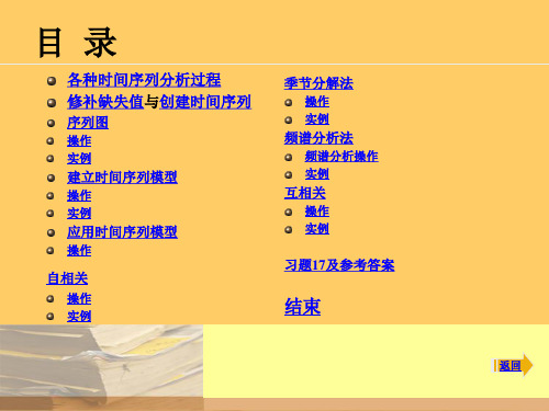
目 录
各种时间序列分析过程 修补缺失值与创建时间序列
序列图
操作 实例
季节分解法
操作 实例
频谱分析法
频谱分析操作 实例
建立时间序列模型
操作 实例
互相关
操作 实例
应用时间序列模型
操作
自相关
操作 实例
习题17及参考答案
结束
返回
各种时间序列分析过程
返回
修补缺失值过程与对话框
返回
时间序列习题参考答案(5)
三、自相关分析
返回
时间序列习题参考答案(6)
表中显示的是自相关计算结果,从左向右,依次列出的是:滞后数、自相关系数 值值、标准误差、Box-ljung统计量(值、自由度、原假设成立的概率值)。由于原假 设(假设基本过程是独立的,也即假定时间序列所反映的随机过程是白噪声)成立的 概率值都小于0.05,所以全部自相关均有显著性意义。
返回
时间序列习题参考答案(17)
六、数据转换
返回
时间序列习题参考答案(18)
返回
spss(时间序列分析)

• 横截面数据也常称为变量的一个简单随机样本,也即假设每个数据 都是来自于总体分布的一个取值,且它们之间是相互独立的(独立 同分布)。
• 而时间序列的最大特点是观测值并不独立。时间序列的一个目的
是用变量过去的观测值来预测同一变量的未来值。 • 下面看一个时间序列的数据例子。 • 例1. 某企业从1990年1月到2002年12月的月销售数据(单位:百
三、指数平滑模型
• 时间序列分析的一个简单和常用的预测模型叫做指数平滑
(exponential smoothing)模型。
• 指数平滑只能用于纯粹时间序列的情况,而不能用于含有独立变量 时间序列的因果关系的研究。
• 指数平滑的原理为:利用过去观测值的加权平均来预测未来的 观测值(这个过程称为平滑),且离现在越近的观测值要给以越重
Seanal adjusted series SA
Seas factors SF
YEAR
图3 销售数据的季节因素分离
第十七页,共70页。
120
可以看出,逐月的销
100 售额大致沿一个指数
80 曲线呈增长趋势。
60
↘
40
20
0
-20 1990 1991 1992 1993 1994 1995 1996 1997 1998 1999 2000 2001 2002
3. saf_1:季节因素(seasonal factor) ,记为{SFt }; 4. stc_1:去掉季节及随机扰动后的趋势及循环因素(trend-
cycle series),记为{TCt }。
第十五页,共70页。
• 这些分解出来的序列或成分与原有时间序列 之间有如下的简单和差关系:
时间序列(ARIMA)案例超详细讲解

想象一下,你的任务是:根据已有的历史时间数据,预测未来的趋势走向。
作为一个数据分析师,你会把这类问题归类为什么?当然是时间序列建模。
从预测一个产品的销售量到估计每天产品的用户数量,时间序列预测是任何数据分析师都应该知道的核心技能之一。
常用的时间序列模型有很多种,在本文中主要研究ARIMA模型,也是实际案例中最常用的模型,这种模型主要针对平稳非白噪声序列数据。
时间序列概念时间序列是按照一定的时间间隔排列的一组数据,其时间间隔可以是任意的时间单位,如小时、日、周月等。
通过对这些时间序列的分析,从中发现和揭示现象发展变化的规律,并将这些知识和信息用于预测。
比如销售量是上升还是下降,是否可以通过现有的数据预测未来一年的销售额是多少等。
1 ARIMA(差分自回归移动平均模型)简介模型的一般形式如下式所示:1.1 适用条件●数据序列是平稳的,这意味着均值和方差不应随时间而变化。
通过对数变换或差分可以使序列平稳。
●输入的数据必须是单变量序列,因为ARIMA利用过去的数值来预测未来的数值。
1.2 分量解释●AR(自回归项)、I(差分项)和MA(移动平均项):●AR项是指用于预测下一个值的过去值。
AR项由ARIMA中的参数p定义。
p值是由PACF图确定的。
●MA项定义了预测未来值时过去预测误差的数目。
ARIMA中的参数q代表MA项。
ACF图用于识别正确的q值●差分顺序规定了对序列执行差分操作的次数,对数据进行差分操作的目的是使之保持平稳。
ADF可以用来确定序列是否是平稳的,并有助于识别d值。
1.3 模型基本步骤1.31 序列平稳化检验,确定d值对序列绘图,进行ADF 检验,观察序列是否平稳(一般为不平稳);对于非平稳时间序列要先进行d 阶差分,转化为平稳时间序列1.32 确定p值和q值(1)p 值可从偏自相关系数(PACF)图的最大滞后点来大致判断,q 值可从自相关系数(ACF)图的最大滞后点来大致判断(2)遍历搜索AIC和BIC最小的参数组合1.33 拟合ARIMA模型(p,d,q)1.34 预测未来的值2 案例介绍及操作基于1985-2021年某杂志的销售量,预测某商品的未来五年的销售量。
以数学建模竞赛为例基于SPSS建立ARIMA模型
以数学建模竞赛为例基于SPSS建立ARIMA模型ARIMA模型是一种时间序列的分析方法,可以用来对未来一段时间内的序列数据进行预测和分析,常常被应用于经济、金融、气象、流行病等领域。
在数学建模竞赛中,ARIMA模型也是常见的分析方法之一。
本文将以数学建模竞赛为例,介绍如何基于SPSS软件建立ARIMA模型。
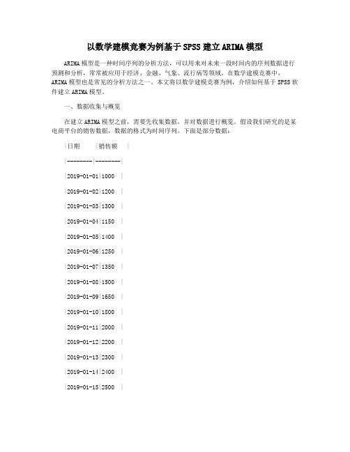
一、数据收集与概览在建立ARIMA模型之前,需要先收集数据,并对数据进行概览。
假设我们研究的是某电商平台的销售数据,数据的格式为时间序列。
下面是部分数据:|日期 |销售额 ||--------|--------||2019-01-01|1000 ||2019-01-02|1200 ||2019-01-03|1300 ||2019-01-04|1150 ||2019-01-05|1400 ||2019-01-06|1250 ||2019-01-07|1350 ||2019-01-08|1500 ||2019-01-09|1650 ||2019-01-10|1800 ||2019-01-11|2000 ||2019-01-12|2200 ||2019-01-13|2300 ||2019-01-14|2400 ||2019-01-15|2500 |通过对数据的概览,我们可以看到销售额有逐渐增加的趋势,并且在一周内出现周期性的波动。
二、建立ARIMA模型1. 模型选择在建立ARIMA模型之前,需要先选择合适的模型。
ARIMA模型的选择最好基于时间序列的图形表示,以及ACF和PACF的分析。
可以通过以下步骤进行模型选择:① 绘制时序图,观察数据的整体趋势、周期变化和异常点等信息。
在SPSS中绘制时序图的方法是:点击菜单Data→Time Series→Line Chart,然后在弹出的对话框中选择“Month-Year”并勾选数据和选项,即可绘制出时序图。
② 绘制ACF和PACF的图形,观察自相关性和偏自相关性。
spss时间序列分析教程

3.3时间序列分析3.3.1时间序列概述1.基本概念(1)一般概念:系统中某一变量的观测值按时间顺序(时间间隔相同)排列成一个数值序列,展示研究对象在一定时期内的变动过程,从中寻找和分析事物的变化特征、发展趋势和规律。
它是系统中某一变量受其它各种因素影响的总结果。
(2)研究实质:通过处理预测目标本身的时间序列数据,获得事物随时间过程的演变特性与规律,进而预测事物的未来发展。
它不研究事物之间相互依存的因果关系。
(3)假设基础:惯性原则。
即在一定条件下,被预测事物的过去变化趋势会延续到未来。
暗示着历史数据存在着某些信息,利用它们可以解释与预测时间序列的现在和未来。
近大远小原理(时间越近的数据影响力越大)和无季节性、无趋势性、线性、常数方差等。
(4)研究意义:许多经济、金融、商业等方面的数据都是时间序列数据。
时间序列的预测和评估技术相对完善,其预测情景相对明确。
尤其关注预测目标可用数据的数量和质量,即时间序列的长度和预测的频率。
2.变动特点(1)趋势性:某个变量随着时间进展或自变量变化,呈现一种比较缓慢而长期的持续上升、下降、停留的同性质变动趋向,但变动幅度可能不等。
(2)周期性:某因素由于外部影响随着自然季节的交替出现高峰与低谷的规律。
(3)随机性:个别为随机变动,整体呈统计规律。
(4)综合性:实际变化情况一般是几种变动的叠加或组合。
预测时一般设法过滤除去不规则变动,突出反映趋势性和周期性变动。
3.特征识别认识时间序列所具有的变动特征,以便在系统预测时选择采用不同的方法。
(1)随机性:均匀分布、无规则分布,可能符合某统计分布。
(用因变量的散点图和直方图及其包含的正态分布检验随机性,大多数服从正态分布。
)(2)平稳性:样本序列的自相关函数在某一固定水平线附近摆动,即方差和数学期望稳定为常数。
样本序列的自相关函数只是时间间隔的函数,与时间起点无关。
其具有对称性,能反映平稳序列的周期性变化。
特征识别利用自相关函数ACF:ρk=γk/γ0其中γk是y t的k阶自协方差,且ρ0=1、-1<ρk<1。
SPSS时间序列分析spss操作步骤
17 习题
1、 时间序列的基本概念。 时间序列分析过程中有哪几种常用的方法?2、 对数据用时间序列模型进行拟合处理前,应做哪些准备工作?3、 在哪个过程中可进行缺失值的修补?修补缺失值的方法共有几种?4、 在哪个过程中可定义时间变量?5、 时间序列分析是建立在序列的平稳的条件上的,怎样判断序列是否平稳?6、为什么要建一个时间序列的新变量?在SPSS的哪个过程中来建时间序列的新变量?7、光盘中Data17-07.sav(Data17-07a.sav是Data17-07.sav使用中文标签名的同一个文件)记录了一个邮购公司在1989年1月至1998年12月间男、女服装产品的销售量情况以及一些可能影响服装销售的宣传、服务方面的变量。试用学过的时间序列方法对其进行分析,并预测1999年4月的男装的销售量。
返回
时间序列习题参考答案(5)
三、自相关分析
返回
时间序列习题参考答案(6)
表中显示的是自相关计算结果,从左向右,依次列出的是:滞后数、自相关系数值值、标准误差、Box-ljung统计量(值、自由度、原假设成立的概率值)。由于原假设(假设基本过程是独立的,也即假定时间序列所反映的随机过程是白噪声)成立的概率值都小于0.05,所以全部自相关均有显著性意义。
返回
时间序列分析实例输出(2)
模型统计数据
返回
时间序列分析实例输出(3)
预测部分结果
数据编辑器中的新变量
返回
应用时间序列模型
(Applies models对话框
返回
自相关
(Autocorrelations )
返回
Autocorrelations对话框
感谢您的下载观看
返回
时间序列习题参考答案(17)
spss时间序列分析教程
3.3时间序列分析3.3.1时间序列概述1.基本概念(1)一般概念:系统中某一变量的观测值按时间顺序(时间间隔相同)排列成一个数值序列,展示研究对象在一定时期内的变动过程,从中寻找和分析事物的变化特征、发展趋势和规律。
它是系统中某一变量受其它各种因素影响的总结果。
(2)研究实质:通过处理预测目标本身的时间序列数据,获得事物随时间过程的演变特性与规律,进而预测事物的未来发展。
它不研究事物之间相互依存的因果关系。
(3)假设基础:惯性原则。
即在一定条件下,被预测事物的过去变化趋势会延续到未来。
暗示着历史数据存在着某些信息,利用它们可以解释与预测时间序列的现在和未来。
近大远小原理(时间越近的数据影响力越大)和无季节性、无趋势性、线性、常数方差等。
(4)研究意义:许多经济、金融、商业等方面的数据都是时间序列数据。
时间序列的预测和评估技术相对完善,其预测情景相对明确。
尤其关注预测目标可用数据的数量和质量,即时间序列的长度和预测的频率。
2.变动特点(1)趋势性:某个变量随着时间进展或自变量变化,呈现一种比较缓慢而长期的持续上升、下降、停留的同性质变动趋向,但变动幅度可能不等。
(2)周期性:某因素由于外部影响随着自然季节的交替出现高峰与低谷的规律。
(3)随机性:个别为随机变动,整体呈统计规律。
(4)综合性:实际变化情况一般是几种变动的叠加或组合。
预测时一般设法过滤除去不规则变动,突出反映趋势性和周期性变动。
3.特征识别认识时间序列所具有的变动特征,以便在系统预测时选择采用不同的方法。
(1)随机性:均匀分布、无规则分布,可能符合某统计分布。
(用因变量的散点图和直方图及其包含的正态分布检验随机性,大多数服从正态分布。
)(2)平稳性:样本序列的自相关函数在某一固定水平线附近摆动,即方差和数学期望稳定为常数。
样本序列的自相关函数只是时间间隔的函数,与时间起点无关。
其具有对称性,能反映平稳序列的周期性变化。
特征识别利用自相关函数ACF:ρk=γk/γ0其中γk是y t的k阶自协方差,且ρ0=1、-1<ρk<1。
- 1、下载文档前请自行甄别文档内容的完整性,平台不提供额外的编辑、内容补充、找答案等附加服务。
- 2、"仅部分预览"的文档,不可在线预览部分如存在完整性等问题,可反馈申请退款(可完整预览的文档不适用该条件!)。
- 3、如文档侵犯您的权益,请联系客服反馈,我们会尽快为您处理(人工客服工作时间:9:00-18:30)。
第七步:设置图表 建议在拟合值出画勾。这样可以鲜明看到拟合值与预测值的比较
第八步:保存选项 在预测值处画勾,并将‘预测值(p)’改为‘预测值’
第九步:选项栏,点击第二个选项,如果定义了日期,则日期处填写想 要预测日期的最后一个日期;如果没有定义日期,则看已知数据的个数, 加上自己要预测的个数,键入即可。 最后点击确定。
结果:如图所示 数据集处:
输出查看器:
输出查看器
预测值
输出查看器的图形
利用
spss17.0
专家建模器 实现 ··· ···
的
时间序列分析
第一步:打开spss17.0的主程序。 打开后的界面如下:
第二步,数据的导入,可以是excel文件,也可以直接复制粘贴过来。这 里以excel的源文件为例。 文件——打开 ;界面如下
打开后的界面如下:
第三步:用时间序列分析 分析——预测——创建模型 界面如下,提示的定义日期可以根据数据的日期格式定义, 不定义也可
可无。
此处仅选x1进行分析,放到因变量的栏里 如下图:
第五步:可以在界面的中间找到条件选项点开:
点开条件选项,可以选择模型类别,默认的为‘所有模型’, 此处以arima模型为例。
在条件选项下还可以选择对离群值的设置。
第六步:设置统计量,注意要在显示预测值的空白处画勾,