数据,模型与决策练习题含答案

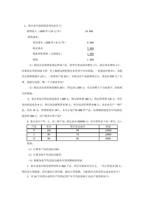
1、某企业目前的损益状况如在下：销售收入（1000件×10元/件）10 000销售成本：变动成本（1000件×6元/件） 6 000固定成本 2 000销售和管理费（全部固定） 1 000利润 1 000（1）假设企业按国家规定普调工资，使单位变动成本增加4％，固定成本增加1％，结果将会导致利润下降。

为了抵销这种影响企业有两个应对措施：一是提高价格5％，而提价会使销量减少10％；二是增加产量20％，为使这些产品能销售出去，要追加500元广告费。

请做出选择，哪一个方案更有利？（2）假设企业欲使利润增加50％，即达到1 500元，可以从哪几个方面着手，采取相应的措施。

2、某企业每月固定制造成本1 000元，固定销售费100元，固定管理费150元；单位变动制造成本6元，单位变动销售费0.70元，单位变动管理费0.30元；该企业生产一种产品，单价10元，所得税税率50％；本月计划产销600件产品，问预期利润是多少?如拟实现净利500元，应产销多少件产品?3、某企业生产甲、乙、丙三种产品，固定成本500000元，有关资料见下表（单位：元）：要求：（1）计算各产品的边际贡献；（2）计算加权平均边际贡献率；（3）根据加权平均边际贡献率计算预期税前利润。

4、某企业每年耗用某种材料3 600千克，单位存储成本为2元，一次订货成本25元。

则经济订货批量、每年最佳订货次数、最佳订货周期、与批量有关的存货总成本是多少？5．有10个同类企业的生产性固定资产年平均价值和工业总产值资料如下：（2）建立直线回归方程；（3）估计生产性固定资产（自变量）为1100万元时总产值（因变量）的可能值。

6、某商店的成本费用本期发生额如表所示，采用账户分析法进行成本估计。

首先，对每个项目进行研究，根据固定成本和变动成本的定义及特点结合企业具体情况来判断，确定它们属于哪一类成本。

例如，商品成本和利息与商店业务量关系密切，基本上属于变动成本；福利费、租金、保险、修理费、水电费、折旧等基本上与业务量无关，视为固定成本。

其次，剩下的工资、广告和易耗品等与典型的两种成本性态差别较大，不便归入固定成本或变动成本。

对于这些混合成本，要使用工业工程法、契约检查法或历史成本分析法，寻找一个比例，将其分为固定和变动成本两部分。

7、某企业每年耗用某种材料3 600千克，单位存储成本为2元，一次订货成本25元。

则经济订货批量、每年最佳订货次数、最佳订货周期、与批量有关的存货总成本是多少？8、某生产企业使用A零件，可以外购，也可以自制。

如果外购，单价4元，一次订货成本10元：如果自制，单位成本3元，每次生产准备成本600元。

每日产量50件。

零件的全年需求量为3 600件，储存变动成本为零件价值的20％，每日平均需求最为10件。

下面分别计算零件外购和自制的总成本，以选择较优的方案。

9 请建立最简单的单阶段存贮模型，推导出经济批量公式，要求说明模型成立的假设条件，所用字母的经济意义，并要有一定的推理过程。

10 若某工厂每年对某种零件的需要量为10000件，订货的固定费用为2000元，采购一个零件的单价为100元，保管费为每年每个零件20元，求最优订购批量。

11 某厂对某种材料的全年需要量为1040吨，其单价为1200元/吨。

每次采购该种材料的订货费为2040元，每年保管费为170元/吨。

试求工厂对该材料的最优订货批量、每年订货次数。

12 某货物每周的需要量为2000件，每次订货的固定费用为15元，每件产品每周保管费为0.30元，求最优订货批量及订货时间。

13 加工制作羽绒服的某厂预测下年度的销售量为15000件，准备在全年的300个工作日内均衡组织生产。

假如为加工制作一件羽绒服所需的各种原材料成本为48元，又制作一件羽绒服所需原料的年存贮费为其成本的22%，提出一次订货所需费用为250元，订货提前期为零，不允许缺货，试求经济订货批量。

14 一条生产线如果全部用于某种型号产品生产时，其年生产能力为600000台。

据预测对该型号产品的年需求量为260000台，并在全年内需求基本保持平衡，因此该生产线将用于多品种的轮番生产。

已知在生产线上更换一种产品时，需准备结束费1350元，该产品每台成本为45元，年存贮费用为产品成本的24%，不允许发生供应短缺，求使费用最小的该产品的生产批量。

15 某生产线单独生产一种产品时的能力为8000件／年，但对该产品的需求仅为2000件／年，故在生产线上组织多品种轮番生产。

已知该产品的存贮费为60元／年·件，不允许缺货，更换生产品种时，需准备结束费300元。

目前该生产线上每季度安排生产该产品500件，问这样安排是否经济合理。

如不合理，提出你的建议，并计算你建议实施后可能带来的节约。

16某电子设备厂对一种元件的需求为R＝2000件/年，订货提前期为零，每次订货费为25元。

该元件每件成本为50元，年存储费为成本的20％。

如发生缺货，可在下批货到达时补上，但缺货损失费为每件每年30元。

求：（1）经济订货批量及全年的总费用；（2）如不允许发生缺货，重新求经济订货批量，并同（1）的结果进行比较。

17 某出租汽车公司拥有2500辆出租车，均由一个统一的维修厂进行维修。

维修中某个部件的月需量为8套。

每套价格8500元。

已知每提出一次订货需订货费1200元，年存贮费为每套价格的30％，订货提前期为2周。

又每台出租车如因该部件损坏后不能及时更换每停止出车一周，损失为400元，试决定该公司维修厂订购该种部件的最优策略。

18 对某产品的需求量服从正态分布，已知μ＝150，σ＝25。

又知每个产品的进价为8元，售价为15元，如销售不完全按每个5元退回原单位。

问该产品的订货量应为多少个，使预期的利润为最大。

19 用图解法求解下列线性规划问题，并指出各问题是具有唯一最优解、无穷多最优解、无界解或无可行解。

(1) min z ＝6x1＋4x2(2) max z ＝4x1＋8x2st. 2x1＋x2≥1 st. 2x1＋2x2≤103x1＋4x2≥1.5 －x1＋x2≥8x1, x2≥0 x1, x2≥0(3) max z ＝x1＋x2(4) max z ＝3x1－2x2st. 8x1＋6x2≥24 st. x1＋x2≤14x1＋6x2≥－12 2x1＋2x2≥42x2≥4 x1, x2≥0x1, x2≥0(5) max z ＝3x1＋9x2(6) max z ＝3x1＋4x2st. x1＋3x2≤22 st. －x1＋2x2≤8－x1＋x2≤4 x1＋2x2≤12x2≤6 2x1＋x2≤162x1－5x2≤0 x1, x2≥0x1, x2≥020、用图解法求解以下线性规划问题：max z= x1+3x2s.t. x1+x2≤10-2x1+2x2≤12x1≤7x1, x2≥021、用图解法求解以下线性规划问题：min z= x1-3x2s.t. 2x1-x2≤4x1+x2≥3x2≥5x1≤4x1, x2≥022、按下表提供的条件绘制箭线型网络图, 计算结点时间参数，并说明作业F、I的最早结束时间和最迟开始时间；求出关键路线。

23根据有关资料预测各状态发生的概率依次为0.3，0.4，0.3，请用决策树法求解此问题。

24、获得大学毕业学位的毕业生，“双向选择”时，用人单位与毕业生都有各自的选择标准和要求。

就毕业生来说选择单位的标准和要求是多方面的，例如：①能发挥自己的才干为国家作出较好贡献（即工作岗位适合发挥专长）；②工作收入较好（待遇好）；③生活环境好（大城市、气候等工作条件等）；④单位名声好（声誉-Reputation）；⑤工作环境好（人际关系和谐等）⑥发展晋升（promote, promotion）机会多（如新单位或单位发展有后劲）等。

问题：现在有多个用人单位可供他选择，因此，他面临多种选择和决策，问题是他将如何作出决策和选择？（运用AHP）1、解：（1）调资后的利润为：1000×[10－6×（1＋4%）]－3000×（1＋10%）＝730元方案一利润为：1000×（1－10%）×[10×（1＋5%）－6×（1＋4%）]－3000×（1＋1%）＝804元方案二利润为：1000×（1＋20%）[10－6×（1＋4%）]－[3000×（1＋1%）＋500]＝982元综上可知，选择方案二更有利。

（2）假设企业欲使利润增加50％，即达到1 500元，可以从以下四个方面着手。

①减少固定成本将固定成本（FC）作为未知数，目标利润1500元作为已知数，其他因素不变，代入本量利关系方程式：1500＝1000×10－1000×6－FC可得FC＝2500元如其他条件不变，将固定成本由3000元减少到2500元，降低16.7%，可保证实现目标利润。

②减少变动成本同上述方法，将变动成本（VC）作为未知数代入本量利关系方程式：1500＝1000×10－1000×VC－3000可得VC＝5.50元如其他条件不变，将变动成本由6元减少到5.50元，降低8.3%，可保证实现目标利润。

③提高售价同上述方法，将单位产品的售价（SP）作为未知数代入本量利关系方程式：1500＝1000×SP－1000×6－3000可得SP＝10.50元如其他条件不变，将单位产品售价由10元提升到10.50元，提高5%，可保证实现目标利润。

④增加产销量同上述方法，将产销数量（V）作为未知数代入本量利关系方程式：1500＝V×10－V×6－3000可得V＝1125件如其他条件不变，将产销量由1000件增加到1125件，提高12.5%，可保证实现目标利润。

2、解：预期利润=10×600－（6＋0.7＋0.3）×600－（1000＋100＋150）＝550元设产销X件产品可实现净利500元则：利润总额为500÷（1－50%）＝1000元10X－（6＋0.7＋0.3）X－（1000＋100＋150）＝1000得X＝750答：预期利润是550元。

如拟实现净利500元，应产销750件产品。

3、解：（1）甲产品的边际贡献＝12000×（100－80）＝240000元乙产品的边际贡献＝15000×（90－75）＝225000元丙产品的边际贡献＝8000×（95－80）＝120000元（2）甲产品销售收入＝12000×100＝1200000元乙产品销售收入＝15000×90＝1350000元丙产品＝8000×95＝760000元总的销售收入＝1200000＋1350000＋760000＝3310000元总的边际贡献＝240000＋225000＋120000＝585000元加权平均边际贡献率＝585000÷3310000×100%＝17.67%（3）预期税前利润＝总的销售收入×加权平均边际贡献率－固定成本＝3310000×17.67%－500000＝84877元答：（1）甲产品的边际贡献为240000元，乙产品的边际贡献为225000元，丙产品的边际贡献为120000元。