脉动风时程matlab程序
B类风场与台风风场下输电塔的风振响应和风振系数
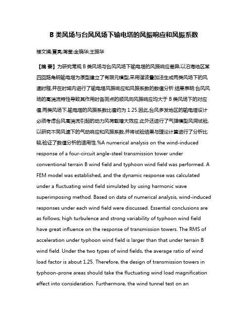
B类风场与台风风场下输电塔的风振响应和风振系数楼文娟;夏亮;蒋莹;金晓华;王振华【摘要】为研究常规B类风场与台风风场下输电塔的风振响应差异,以沿海地区某四回路角钢输电塔为原型建立了有限元模型,采用谐波叠加法生成两类风场下的风速时程,并在时域内进行了输电塔风振响应和风振系数的数值分析.结果表明:台风风场的高湍流特性导致其作用时各测点的顺风向风振响应均大于B类风场下的对应值.两类风场下,输电塔的风振系数比值约为1.25.因此,台风多发地区的输电塔设计必须考虑台风高湍流引起的动力风荷载增大效应.此外还进行了气弹模型风洞试验,以研究不同风速下的气动响应和风振系数,并将试验结果与理论计算进行了分析比较,验证了数值分析的适用性.%A numerical analysis on the wind-induced response of a four-circuit angle-steel transmission tower under conventional terrain B wind field and typhoon wind field was performed. A FEM model was established, and the dynamic response was calculated under a fluctuating wind field simulated by using harmonic wave superimposing method. Based on data of numerical analysis, wind-induced responses under each wind field were discussed. Essential conclusions are as follows; high turbulence and strong variability of typhoon wind field have great influence on the response of transmission towers. The RMS of acceleration under typhoon wind field is larger than that under terrain B wind field. Under the two types of wind fields, the average ratio of wind load factor is about 1.25. Therefore, the design of transmission towers in typhoon-prone areas should take the fluctuating wind load magnification effect into consideration. Furthermore, the wind tunnel test on anaeroelastic model of the transmission tower was performed to study its wind-induced responses under different velocity. The test results were compared with theoretical values and the accuracy of the numerical analysis was verified.【期刊名称】《振动与冲击》【年(卷),期】2013(032)006【总页数】5页(P13-17)【关键词】输电塔;数值分析;风振响应;风振系数;台风风场【作者】楼文娟;夏亮;蒋莹;金晓华;王振华【作者单位】广东省电力设计研究院,广州510663【正文语种】中文【中图分类】TU973.32我国东南沿海为台风多发地区,台风风场的高湍流度、强离散性和强变异性等特征将产生与良态风作用下不同的复杂风振效应,而现行规范尚未涉及台风作用下输电塔风荷载的具体规定。
脉冲发生器matlab程序

function p=pulsegen(fs,T,edge,type,f,opt);%p=pulsegen(fs,T,edge,type,f,opt);%a signal generation program%fs is the sampling frequency%T is the total signal length%edge is a decay parameter for some waveforms% it is used in 'gaussian', 'monocycle', 'biexponential', 'mexican hat', 'sinc', 'double sinc', 'sinc squared'% and windowed sweep% it is mostly a parameter to describe how much the edge of the pulse is decayed.%type is the type of the waveform desired% allowable types are 'gaussian', 'square', 'triangle', 'monocycle',% 'biexponential', 'mexican hat', 'sinc', 'double sinc', 'sinc squared','sweep', and 'windowed sweep'%f is the modulation frequency if left out it is assumed 0.%opt is an optional argument for pulse waveforms requiring a lower and higher frequency% it is used in 'double sinc' ,'sweep' and 'windowed sweep' for the low and high frequency.% the pulses are always normalized to a peak amplitude of 1if nargin<4 %test for optional argumentserror('not enough input arguments');elseif nargin==4f=0;opt=[16*edge/(5*T),64*edge/(5*T)];elseif nargin==5opt=[16*edge/(5*T),64*edge/(5*T)];endif (edge==0)edge==1;endt=-T/2:1/fs:T/2;sig=(T/8/edge)^2;switch typecase {'guassian'} %generate a guassian pulsey=exp(-(t).^2/sig);case {'square'} %generate a square pulsey=ones(size(t));case {'triangle'} %generate a triangle pulsey=(t+T/2).*(t<0)-(t-T/2).*(t>=0);case {'monocycle'} %generate a gaussian monocycley=2*t./sig.*exp(-(t).^2/sig);case {'biexponential'} %generate a biexponential pulsey=exp(-abs(t)*8*edge/T);case {'mexican hat'} %generate a gaussian second deriviativez=t./sqrt(0.75*sig);y=sqrt(1/2*pi).*(1-z.^2).*exp(-z.^2/2);case {'sinc'} %generate a sinc functiony=sinc(2*pi*edge*16.*t/(5*T));case {'double sinc'} %generate a bandlimited function from two sinc functions y=opt(1)*sinc(2*opt(1).*t)-opt(2)*sinc(2*opt(2).*t);case {'sinc squared'} %generates sinc squared functiony=sinc(2*pi*edge*16.*t/(5*T)).^2;case {'sweep'} %generate frequency sweeptheta=(opt(1)+(opt(2)-opt(1))/T).*(t+T/2);y=real(exp(j*(theta.*(t+T/2)-pi/2)));case {'windowed sweep'} %generate a windows frequency sweeptheta=(opt(1)+(opt(2)-opt(1))/T).*(t+T/2);y=real(exp(j*(theta.*(t+T/2)-pi/2)));c=length(y);edge=min(1,edge);edge=max(0,edge);w=hamming(ceil(c*(1-edge)));w2=[w(1:ceil(length(w)/2));ones(c-length(w),1);w(ceil(length(w)/2)+1:end)]';y=w2.*y;otherwiseerror('invalid pulse type');end%apply a modulationif f~=0y=y.*cos(2*pi*t*f);end%normalize the peak of the pulse to 1p=y./max(abs(y));。
脉动风的数值模拟

公 路一 I 级设 计荷 载标 准要求 。 《 公路 桥梁 承 载 能 力 检 测评 定 规 程 》 规定 , 主 要控 制测 点 的相对残 余应 变 和相 对残余 挠 度不 大 于2 O , 实测 数 据 换 算 结 果 表 明 , 实 测 相 对 残 余
[ s ] . 北京 : 人 民交 通 出 版 社 , 2 0 1 1 .
特征 , 以及 脉 动 风 国 内 外 几 种 常用 的 模 拟 方 法 , 阐述其数值模 拟理论 , 根据 所选用 的线性滤波法 , 结 合 京 包 铁 路 分 离式 立交 桥 桥 址 处 气 象 资 料 , 用 MA TL A B软 件 编 程 模 拟 脉 动 风 , 并 得 到 风 速 时 程 曲线 , 将 模 拟 出 的 功 率 谱 与 目标 谱 对 比其 拟 合 度 , 结 果表 明, 模 拟 谱 与 目标 谱 吻 合 度 较 高 , 模 拟 的
结果较为可靠 。
关 键 词 平 均 风 脉 动风 数 值 模 拟 线 风 由于 带 有 随 机 的 特 性 , 不 利 于研 究 。 通常 在研 究 自然风 时可 以将 其分 解为 平均 风 和脉
动风 , 视 为 两 者 的叠 加 。
起 主要 作用 的有 地 面粗糙 度标 准 、 重现期 、 时距标 准 与 高度标 准 。我 国规定 的风 速测 量标 准 高度定
为 1 0 I T I , 平 均时距 取 为 l O mi n , 年最 大风 速重 现
*内 蒙 古 自治 区 交 通 科技 项 目( N J 一 2 0 1 2 - 1 8 ) 资 助 收 稿 日期 : 2 0 1 4 — 0 3 — 2 3
3 0
黄 伟 文 张 谢 东 : 脉 动 风 的 数 值 模 拟
基于Newmark-β法的Matlab简单程序编写

的 差 分 , 根 据 初 始 条 件 并 利 用 直 接 积 分 法 ,逐步求 系列离散 上 的 响 应 值 ,迄 今 为 止 ,已 许 多 研 究 者
提出了多种不同的离散化差分 。例 如 ,线性加速 及
其 广 义 形 式 的 Newmark - p 法 、[ilson - 0 法 、中 央 差 分 法 、
Newmark - p 法是求解结构动力学冋题最常用也是最为
广泛的方法,因 为 Newmak - p 法 的 逻 辑 性 强 、理论较为简
单 。其理论的条理性也
程序 的 编写。朱 清 [3]
已 证 明 Newmark - b 法 当 2 p " - " 1 / 2 时是无条件稳定的,即
当 p = - = 1 / 2 时 。下 面 笔 者 将 对 Newmak - p 法理论进行
收稿日期:2018 -03 -19 作者简介: (1994 - " ,男,四川南充人,在读硕士研究生,主要 研究 :大 连续梁桥。
取为 距的 步 长 。在每个
隔的起点和 建
程 ,并 个 假 设 的 反 应 机 理 为 根 据 ,近似地
计算在
隔内体系的运动(通 略在
隔生
的 不 ),体系的 所 的当 形
Xiliua university, Chengdu 610039,China) Abstract %[ e know that it is much difficult to directly solve the problems of the structural dynamics, but the method of Newmark - p can masterly work it down, the method of Newmark - p is a time history analysis.It transform the differential equation to the algebraic equation, it is easy to solve problems.It is an implicit integration which can get the correct answer. In this paper, the author write the code of Matlab program based on the theoretical knowledge of Newmarlc - p to solve a simple question of structur al dynamics. Key words %newmark - p #code of matlab program #stuctural dy namics
matlab练习程序(差分法解一维波动方程)
matlab练 习 程 序 ( 差 分 法 解 一 维 波 动 方 程 )
实现了二维热传导方程数值解,这里我们计算波动方程数值解。 波动方程是一种双曲型偏微分方程。 这里依然用差分法计算。 一维波动方程如下:
写成差分形式:
整理一下就能得到u(i+1,j)。
en meshgrid(0:hx:x,0:ht:t); mesh(x1,t1,u)
结果如下:
matlab代码如下:
clear all;close all;clc;
t = 2;
%时间范围,计算到2秒
x = 1;
%空间范围,0-1米
m = 320;
%时间方向分320个格子
n = 64;
%空间方向分64个格子
ht = t/(m-1); %时间步长dt
hx = x/(n-1); %空间步长dx
u = zeros(m,n);
%设置边界条件 i=2:n-1; xx = (i-1)*x/(n-1); u(1,2:n-1) = sin(2*pi*xx); u(2,2:n-1) = sin(2*pi*xx);
%根据推导的差分公式计算 for i=2:m-1
for j=2:n-1 u(i+1,j) = ht^2*(u(i,j+1)+u(i,j-1)-2*u(i,j))/hx^2 + 2*u(i,j)-u(i-1,j);
采用MATLAB+Simulink的液压管路瞬态压力脉动分析

图3
选择算子 常数
分别加上两个边界条件
p2 p3 Μ p′ = p n p0
则构成两个新的向量
q0 q q′ = 1 Μ qn −1
∂p 在 Simulink 中的表达方式 ∂x ∂p Fig.3 Simulink diagram of ∂x
整个管路动态压力脉动特性分析的 Simulink 仿 真块图如图 4 所示 其中子系统 subsystem 为包括 稳态项和瞬态项的摩擦力项
常数 2
积分器 1 选择算子 2
选择算子 1 常数 1 积分器 2
子系统
图4 Fig.4
Simulink 仿真块图
Simulink simulating module 表2 Table 2 仿真参数
q ðr02
=
其中系数 ni 和 mi 采用日本研究人员 KAGAWA 给 出的数值[5] 如表 1 所示
表1 Table 1 系数 ni 和 mi 值
Coefficients ni and mi
t
1 2 3 4 5 6 7 8 9 10
ni
2.63744×101 7.28033×101 1.87424×10² 5.36626×10² 1.57060×10³ 4.61813×10³ 1.36011 ×10⁴ 4.00825×10⁴ 1.18153×10⁵ 3.48316×10⁵
Abstract: The mathematical model of fluid transients inside hydraulic pipelines is introduced including the unsteady friction item. A new method using SELECTOR block in MATLAB Simulink is developed to handle the integration in spatial domain when solving the partial differential equations. Using this method, the pressure transients inside hydraulic pipelines can be predicted both in time and spatial domains. A straight pipeline with a hydraulic valve on one side and a reservoir on the other side is studied as an example. The pressure pulsations inside the pipeline after the valve is shut off are simulated using the new method. The simulation results are given and compared with the predictions from characteristics method and finite element method published previously. The high frequency oscillation problem created by the numerical analysis is also discussed. Key words: pressure pulsations; pipeline transients; MATLAB Simulink; hydraulic pipeline; partial differential equation 在石油输送管网系统 航空航天燃油供给系统 以及液压传动系统中 由于阀门的突然开关 泵的 失效以及执行元件止动等原因 管道中将产生沿管 路传播的压力脉动波 这种现象会导致传输 传动 及控制系统性能的下降 例如泵效率的降低 系统
matlab动力学分析程序详解

11.微分方程的定义对于duffing 方程032=++x x x ω,先将方程写作⎩⎨⎧--==3112221x x x x x ω function dy=duffing(t,x) omega=1;%定义参数 f1=x(2);f2=-omega^2*x(1)-x(1)^3; dy=[f1;f2];2.微分方程的求解function solve (tstop) tstop=500;%定义时间长度 y0=[0.01;0];%定义初始条件[t,y]=ode45('duffing',tstop,y0,[]);function solve (tstop) step=0.01;%定义步长y0=rand(1,2);%随机初始条件tspan=[0:step:500];%定义时间范围 [t,y]=ode45('duffing',tspan,y0);3.时间历程的绘制时间历程横轴为t ,纵轴为y ,绘制时只取稳态部分。
plot(t,y(:,1));%绘制y 的时间历程 xlabel('t')%横轴为t ylabel('y')%纵轴为y grid;%显示网格线2axis([460 500 -Inf Inf])%图形显示范围设置4.相图的绘制相图的横轴为y ,纵轴为dy/dt ,绘制时也只取稳态部分。
红色部分表示只取最后1000个点。
plot(y(end-1000:end ,1),y(end-1000:end ,2));%绘制y 的时间历程xlabel('y')%横轴为yylabel('dy/dt')%纵轴为dy/dt grid;%显示网格线5.Poincare 映射的绘制对于不同的系统,Poincare 截面的选取方法也不同对于自治系统一般每过其对应线性系统的固有周期,截取一次 对于非自治系统,一般每过其激励的周期,截取一次例程:duffing 方程032=++x x x ω的poincare 映射 function poincare(tstop)global omega; omega=1;T=2*pi/omega;%线性系统的周期或激励的周期 step=T/100;%定义步长为T/100 y0=[0.01;0];%初始条件tspan=[0:step:100*T];%定义时间范围 [t,y]=ode45('duffing',tspan,y0);for i=5000:100:10000%稳态过程每个周期取一个点 plot(y(i,1),y(i,2),'b.'); hold on;% 保留上一次的图形 endxlabel('y');ylabel('dy/dt');3Poincare 映射也可以通过取极值点得到 function poincare(tstop) y0=[0.01;0];tspan=[0:0.01:500];[t,y]=ode45('duffing',tspan,y0); count=find(t>100);%截取稳态过程 y=y(count,:);n=length(y(:,1));%计算点的总数 for i=2:n-1if y(i-1,1)+eps<y(i,1) && y(i,1)>y(i+1,1)+eps % 简单的取出局部最大值plot(y(i,1),y(i,2),'.'); hold on end endxlabel('y');ylabel('dy/dt');6.频谱yy=fft(y(end-1000:end,1)); N=length(yy); power=abs(yy);freq=(1:N-1)*1/step/N;plot(freq(1:N/2),power(1:N/2)); xlabel('f(y)') ylabel('y')7.算例duffing 方程03=++x x x的时间历程,相图,频谱和poincare 映射。
脉动风荷载时程数值模拟研究
率谱和相关函数这两个 函数来描述脉动风。 1 . 1 常用 风 速功率 谱 脉动风的风速功率谱主要反映脉动风中各种频 率成 分对 应 的能量分 布 规律 。按方 向可 分 为水平 脉 动风速功率谱和垂直脉动风速功率谱 , 目前使用最 广泛 的是水 平风 速功 率谱 , 其中 D a v e n p o r t 谱 、 H a r r i s 谱[ 8 3 不考虑 湍流积 分尺度 随高度 的变化 情
高耸结构 、 大跨度结构等在风荷载作用下的效应 , 对
结 构 的安 全 性和适 用 性甚 至起 着决 定性 的影 响 。在 结 构 设计 计算 考 虑 风荷 载 时 , 除 了在 平 均风 作 用 下 对建 筑结 构 进行 静 力计 算 外 , 有 时 还 需 对 脉 动 风荷 载下 建 筑 结 构 的动 力 响 应 进 行 分 析 … 。 对 于 重 要 的结 构 , 通 常采用 风 洞 试 验 的方 法来 测试 其 动力 响 应, 但风 洞试 验 方法耗 时耗资 巨 大 , 目前 尚无法 在工 程设 计分 析 领域 中普 遍使 用 。而 通过计 算 机模 拟脉 动风 荷 载 , 可 以很 好 地 帮 助 工 程 人 员 掌握 实 际工 程 结 构 的风振 特性 。事 实 上 , 考 虑 到 在 实 际 的 大气 边 界层 紊 流风 场 中 , 脉 动风 速不 仅是 时 间 的函数 , 而且 随 空 间位置 而变 化 , 是 一 个 随机场 , 数值 模 拟方 法反 而 比实 际记 录更 具 有代 表 性 , 因而 在 实 际 工程 中被 广 泛使 用 一 。
况, 而S i m i u谱 、 H i n o谱 、 K a i m a l 谱 等 考 虑 了
- 1、下载文档前请自行甄别文档内容的完整性,平台不提供额外的编辑、内容补充、找答案等附加服务。
- 2、"仅部分预览"的文档,不可在线预览部分如存在完整性等问题,可反馈申请退款(可完整预览的文档不适用该条件!)。
- 3、如文档侵犯您的权益,请联系客服反馈,我们会尽快为您处理(人工客服工作时间:9:00-18:30)。
根据风的记录,脉动风可作为高斯平稳过程来考虑。
观察n 个具有零均值的平稳高斯过 程,其谱密度函数矩阵为:
_Sii ^)気临)...% (灼)]
〜、
S 21(国)S 22(⑷)...S 2n (⑷)
S (CO )= ±1(00)乳儉)…Snn (G0)_
将SC )进行Cholesky 分解,得有效方法。
其中,
T
H C )为H (「)的共轭转置。
根据文献[8],对于功率谱密度函数矩阵为 SC )的多维随机过程向量, 模拟风速具有如 F 形式:
j N
V j ⑴=送 Z ‘H jm ®)|
cosb l t 理 jm ® )P ml ]
m=! l ± j =1,2,3..., n (12)
其中,风谱在频率范围内划分成 N 个相同部分,△⑷=⑷/N 为频率增量,H jm (⑷丨)为 上述
下三角矩阵的模,jm (打)为两个不同作用点之间的相位角, r ml 为介于0和2二之间
均匀分布的随机数, j =|是频域的递增变量。
文中模拟开孔处的来流风,因而只作单点模拟。
即式(
4)可简化为:
N v (t )=送 |H (创)72M cos b |t +d 】
(13)
im 本文采用Davenport 水平脉动风速谱:
2 4kx 2
S v (n )二 V 10 2 473
( 14) n (1 x )
式中,S v (n )――脉动风速功率谱; n ——脉动风频率(Hz ); k ——地面粗糙度系数;
S( ) = H( J H C )T (10)
H (;:;■)= 旳11心)
|H
21(豹)
H
22 C 0 ... Bnlg) H n2( ) ... H nn®) 一 (11)
x =1200_
V10
v10----- 标准高度为10m处的风速(m/s)。
Matlab 程序:
N=10;
d=0.001;
n=d:d:N;%% 频率区间(0.01 〜10)
v10=16;
k=0.005;
x=1200* n/v10;
s1=4*k*v10A2*x.A2./n./(1+x42).A(4/3);%%Dave nport 谱
subplot(2,2,1)
loglog(n,s1)%% 画谱图
axis([-100 15 -100 1000])
xlabel('freq');
ylabel('S');
for i=1:1:N/d
H(i)=chol(s1(i));%%Cholesky 分解
end
thta=2*pi*rand(N/d,1000);%% 介于0和2pi之间均匀分布的随机数t=1:1:1000;%% 时间区间(0.1 〜100s)
for j=1:1:1000
a=abs(H);
b=cos(( n*j/10)+thta(:,j)');
c=sum(a.*b);
v(j)=(2*d).A(1/2)*c;%% 风荷载模拟
end subplot(2,2,2)
plot(t/10,v)%%显示风荷载
xlabel('t(s)');
ylabel('v(t)');
Y=fft(v);%%对数值解作傅立叶变换
Y(1)=[];%%去掉零频量
m=length(Y)/2;%%计算频率个数;
power=abs(Y(1:m)).A2/(le ngth(Y).A2);%% 计算功率谱
freq=10*(1:m)/le ngth(Y);%% 计算频率,因为步长为0.1,而不是1,故乘以10 subplot(2,2,3)
Ioglog(freq,power,'r',n,s1,'b')%% 比较 axis([-100 15 -100 1000]) xlabel('freq');
ylabel('S');
对源程序的修改:
z=xcorr(v);
Y=fft(z);%%对数值解作傅立叶变换
Y(1)=[];%%去掉零频量
m=length(Y)/2;%%计算频率个数;
power=abs(Y(1:m)).A 2/(le ngth(Y).A
2);%% 计算功率谱 freq=10*(1:m)/le ngth(Y);%% 计算频率,因为步长为 0.1,而不是1,故乘以10 subplot(2,2,3) loglog(freq,power,'r',n,s1,'b')%% 比较 axis([-100 15 -100 1000]) xlabel('freq');
ylabel('S');
楼主的修改使模拟得到的功率谱与源谱的数量级对上了,
但是吻合不是太好。
但是好像这样 做是不对的。
求信号x(t)的功率谱有两种方法,一是对
X(t)做傅立叶变换,再平方
S=abs(fft(x))A2 一是先对X(t)求相关系数,再进行傅立叶变换 :
10
freq 10
10
10
t(s)
freq
S=fft(xcorr(X))
楼主的方法好像是这两个方法的混合。
欢迎大家拍砖
freq
i。