Generic, Model-Based Edge Estimation in the Image Surface
Client World Model Synchronous Alignement for Speaker Verification

password phonetic structure is similar for the speaker and the impostors. This motivates the study of a synchronous alignment approach where the hidden process (i.e the sequence of states) is supposed identical for both client and nonclient. Only the output distributions differ between the two hypotheses. The synchronous alignment approach is depicted and compared to the classical one on Figure 1.
The main idea of synchronous alignment is to make the two models share the same topology and differ in the output distributions. In order to compute the optimal path in the shared model, a global criterion is defined. Two possible criteria are proposed in this section. Specific decoding and training algorithms for both criteria are derived. The convergence properties of such algorithm are studied and the results are presented here. 2.1 Criteria for synchronous alignment
特种陶瓷词汇

cubic crystal structure立方晶体结构
cuilet(用于回收利用的)玻璃碎片
cupric oxide氧化铜
cuprous oxide氧化亚铜
curing reaction固化反应,凝固反应
cusp尖顶
cutoff切断,截止
degrade降低,衰变
deleterious有害的,有害杂质
deliberately 慎重地,仔细地,精密地
demarcation划分,划界线
denote表示
departure分离,分开
depth of penetration of the water水
渗入的深度
derive派生
alcohol乙醇,酒精
aldehyde乙醛
algorithm算法,演段
align排列,对齐,调整
Alite阿利特,A矿
alkali-deficient layer缺碱层
alkali(pl.alkalis或alkalies)碱,碱性
calcite 方解石CaC03
calcium sulfate硫酸钙,石膏
calcium carbonate碳酸钙
calcium silicate硅酸钙
calcium钙
calcium sulphate硫酸钙
calcium oxide氧化钙
calcium carbonate碳酸钙
displace排出,把…移开
disposal处理,布置,控制,支配
disrupt断裂,碎裂
dissipate消散,散逸
dissipation消耗,消除,消激
基于跨模态蒸馏的无监督行人重识别算法

DOI :10.15913/ki.kjycx.2024.08.004基于跨模态蒸馏的无监督行人重识别算法陈济远(华中科技大学人工智能与自动化学院,湖北 武汉 430074)摘 要:无监督行人重识别任务要求在训练数据没有标注的情况下训练出能够进行跨摄像头检索的行人重识别模型,如何在缺失行人真实身份标签的情况下训练模型提取出具有鲁棒性和判别性的特征是无监督行人重识别研究的难点。
针对基于文本的跨模态行人重识别中模态间分布差异问题,提出基于跨模态蒸馏的无监督行人重识别算法,通过构建跨模态分类对比损失、跨模态蒸馏损失和模态内规范化损失,在无行人标注的情况下,训练出能够提取具有跨模态不变性和行人身份判别性特征的模型。
关键词:计算机视觉;无监督学习;行人重识别;深度学习中图分类号:TP391.41 文献标志码:A 文章编号:2095-6835(2024)08-0014-05在行人重识别任务的各种变体中,基于文本的跨模态行人重识别任务旨在使用文字描述信息检索具有同一身份的行人图片,主要应用于没有目标行人照片只有相关语言表述的实际场景。
这一设定在无目标行人图像只有语言描述的实际场景中有巨大作用。
近年来,基于监督学习的文本跨模态行人重识别方法已经获得了巨大的提升。
这些方法遵从一个相似的学习框架,即通过行人身份构建文本-图像正负样本对监督跨模态匹配。
这些方法都强烈依赖于行人身份标注,然而行人重识别数据集的标注需要耗费大量人力物力,因此一些研究者提出无需行人身份标注,保留文字和图像间配对关系的基于文本的跨模态无监督行人重识别任务。
尽管在基于文本的跨模态无监督行人重识别任务中,文本和图像的匹配关系被保留,但是由于缺失行人身份信息,存在如下问题:各个模态内行人身份存在特征差异,在缺少行人身份信息监督的情况下很难被消除;在进行跨模态的文本图像匹配时无法精确匹配对应行人。
因此,基于跨模态蒸馏的无监督行人重识别方法是通过使用深度神经网络分别对文本和图像提取的特征进行聚类获取伪标签,使用行人身份伪标签监督模型训练,对数据集进行一整轮训练后重新进行识别[1]。
INRIA Sophia-Antipolis
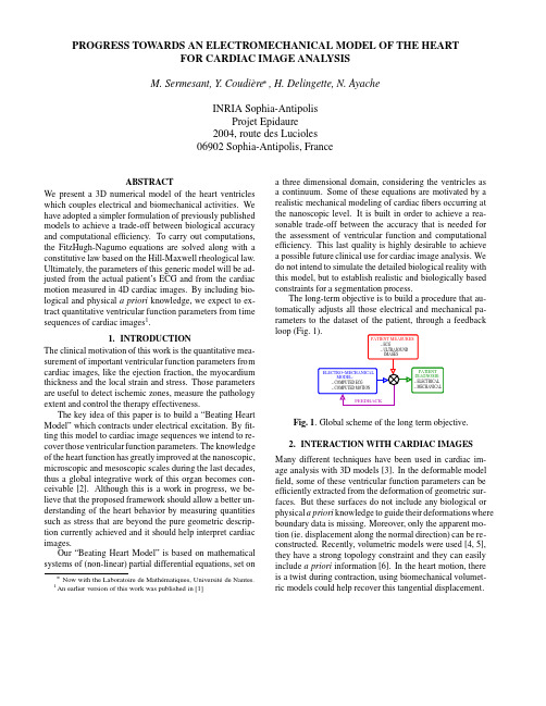
PROGRESS TOWARDS AN ELECTROMECHANICAL MODEL OF THE HEARTFOR CARDIAC IMAGE ANALYSISM.Sermesant,Y.Coudière,H.Delingette,N.AyacheINRIA Sophia-AntipolisProjet Epidaure2004,route des Lucioles06902Sophia-Antipolis,FranceABSTRACTWe present a3D numerical model of the heart ventricleswhich couples electrical and biomechanical activities.Wehave adopted a simpler formulation of previously publishedmodels to achieve a trade-off between biological accuracyand computational efficiency.To carry out computations,the FitzHugh-Nagumo equations are solved along with aconstitutive law based on the Hill-Maxwell rheological law.Ultimately,the parameters of this generic model will be ad-justed from the actual patient’s ECG and from the cardiacmotion measured in4D cardiac images.By including bio-logical and physical a priori knowledge,we expect to ex-tract quantitative ventricular function parameters from timesequences of cardiac images1.1.INTRODUCTIONThe clinical motivation of this work is the quantitative mea-surement of important ventricular function parameters fromcardiac images,like the ejection fraction,the myocardiumthickness and the local strain and stress.Those parametersare useful to detect ischemic zones,measure the pathologyextent and control the therapy effectiveness.The key idea of this paper is to build a“Beating HeartModel”which contracts under electrical excitation.Byfit-ting this model to cardiac image sequences we intend to re-cover those ventricular function parameters.The knowledgeof the heart function has greatly improved at the nanoscopic,microscopic and mesoscopic scales during the last decades,thus a global integrative work of this organ becomes con-ceivable[2].Although this is a work in progress,we be-lieve that the proposed framework should allow a better un-derstanding of the heart behavior by measuring quantitiessuch as stress that are beyond the pure geometric descrip-tion currently achieved and it should help interpret cardiacimages.Our“Beating Heart Model”is based on mathematicalsystems of(non-linear)partial differential equations,set onIn the deformable model framework,a model evolves under the influence of two energies:an External Energy which makes the modelfit the images and an Internal En-ergy which acts as a regularization term and can include a priori information(shape,physical properties,motion,...)Fig.2.Electromechanical model in a4D ultrasound image.In our approach,the computation of this External En-ergy at a surface vertex depends not only on the vertex loca-tion but also on its normal direction.Different type of forces may be applied depending on the image modality.We chose to combine intensity and gradient information with a region-based approach[7]applied to the intensity profile extracted at each vertex in its normal direction.It consists in defin-ing a region with a range of intensity values and thenfind-ing its boundary by looking at the voxels of high gradient value.The extent of the intensity profile is decreased in the coarse-to-fine process.Then,we apply a force which is proportional to the distance to the closest boundary point of the image from the considered point of the mesh surface.The volumetric nature of our model strongly decreases the importance of the image outliers in the motion estima-tion since it strongly constrains the geometric(for instance the thickness of the myocardium wall)and physical behav-ior.The Internal Energy corresponds to an electromechan-ical“Beating Heart Model”which is described in the next three sections:first,the anatomical data necessary to build the model,then the electrical model used to compute the action potential wave propagation andfinally the mechani-cal model used to compute the contraction triggered by the action potential wave.3.ANATOMICAL MODELTo build our model we need data regarding both the3D ven-tricular geometry and the musclefiber directions.Indeed, the anisotropy created by thosefibers intervenes in both the electrical wave propagation and the mechanical contraction. There are different ways to obtain thosefiber directions. We are currently using data from a dissected canine heart available from the Bioengineering Research Group2of the University of Auckland,New Zealand and from reduced-encoding MR diffusion tensor imaging(dtMRI)[8].In order to complete our anatomical model we also need data about the electrical network:the Purkinje network lo-as in[10],or as the result of some equilibrium equations that govern the conducting continuum,like in the so-called bidomain model[12].The anisotropy of the ventricles is taken into account through the diffusion tensor:,in a local orthonormal basis where is parallel to the fiber.is a scalar conductivity and the anisotropy ratio between the transverse and the axial conductivities.4.3.Results of the wave propagationSimulated isochrones of activation are presented(Fig.4),af-ter a wave was initialized at the apex,using a crude approx-imation of the Purkinje network and a slightly anisotropic diffusiontensor.Fig.4.Isochrones of activation(computed with a slightlyanisotropic diffusion tensor:)We can simulate different singularities that may corre-spond to pathologies by changing the conduction parame-ters(Fig.5),for instance introducing a strong conductivityanisotropy.Fig.5.Apparitions of activation singularities with a highlyanisotropic diffusion tensor.This time-dependent computed potential can then be usedas an excitation entry to the system describing the mechan-ical behavior of the myocardium.5.MECHANICAL MODELThe myocardium is composed of musclefiber bundles spi-raling around the two ventricles.It is a nonlinear viscoelas-tic anisotropic active material.The qualitative behavior ofthe electromechanical coupling is a contraction for a pos-itive action potential and an active relaxation for a nega-tive one.Moreover,the action potential also modifies thestiffness of the material.The model introduced in[13,14]by Bestel,Clément and Sorine captures this behavior.Theglobal muscle model is based on the Hill-Maxwell rheolog-ical law which includes a contractile element,a serieselement and a parallel element,as shown on Fig.6and is detailed in[15].EpFig.6.(Left)Hill-Maxwell rheological model.(Right)Simplified rheological model.In[14],Bestel,Clément and Sorine model the contrac-tile element,controlled by the action potential,as fol-lows:around10minutes whereas other existing electromechan-ical models take several hours of computation.We are in-vestigating optimization and a parallel implementation to reduce the computation time to allow an interactive use of this model in time series of cardiac images.The long term goal is to use this model to extract quan-titative parameters of the ventricular function from cardiac images.We can also simulate electrical wave singularities that may correspond to pathologies or test different loca-tions of electrical onset,useful for the implantation of pace-makers,for instance.Moreover,we will be able to simulate the influence of those electrical differences on the contrac-tion.We believe that this beating heart model could help understand the consequences of local electrical or mechan-ical failures on the global motion.Additional images and videos are available on the web3.Globally,recent measurements of the electrical activ-ity,fiber directions and motion reconstruction(from tagged MRI)on the same heart should help adjust the different pa-rameters of the model[16].We will work during the com-ing months on validating this method with an entire dataset coming from the same heart.Finally,a more accurate model may be considered,and different numerical techniques exist:the complete simula-tion process can be improved,always keeping in mind the balance between the complexity of the models(more equa-tions but more realistic)and the efficiency of the numerical methods(accuracy and speed).7.ACKNOWLEDGEMENTSThis work is a part of the multidisciplinary project ICEMA4 (standing for Images of the Cardiac ElectroMechanical Ac-tivity),which is a collaborative research action between dif-ferent INRIA projects and Philips Research France[17].8.REFERENCES[1]M.Sermesant,Y.Coudière,H.Delingette,N.Ayache,andJ.A.Désidéri,“An electro-mechanical model of the heart for cardiac image analysis,”in Medical Image Comput-ing and Computer-Assisted Intervention(MICCAI’01).2001, vol.2208of Lecture Notes in Computer Science(LNCS),pp.224–231,Springer.[2] A.McCulloch,J.B.Bassingthwaighte,P.J.Hunter,D.Noble,T.L.Blundell,and T.Pawson,“Computational biology of the heart:From structure to function,”Progress in Biophysics& Molecular Biology,vol.69,no.2/3,pp.151–559,1998. [3] A.F.Frangi,W.J.Niessen,and M.A.Viergever,“Three-dimensional modeling for functional analysis of cardiac im-ages:A review,”IEEE Trans.on Medical Imaging,vol.1, no.20,pp.2–25,2001.[4]X.Papademetris,A.J.Sinusas,D.P.Dione,and J.S.Dun-can,“Estimation of3D left ventricle deformation from。
临床试验中英对照词汇表english vocabulary of clinical trials-yrn2019051011

首席医学官 首席营销官
国家食品药品监督管理总局
圆二色谱 清除率 临床稽查员 临床数据管理系统 临床总监 临床等效应 临床研究监查助理 临床监查/运营 临床项目助理 临床研究监察员,临床研究助理 临床协调员 临床研究
Page 2
2019/5/10
ENGLISH VOCABULARY OF CLINICAL TRIALS
resolution
数据澄清和解决表
Page 3
2019/5/10
ENGLISH VOCABULARY OF CLINICAL TRIALS
DCF DCR DM DMP DMSF DQF DVP
DF
DSC DFS
DLT
eCRF EDC EDP EOS
EC ESH-ESC
EU EBM
data clarification form
标准批准表格
ALD
approximate lethal dose
近似致死剂量
AUC
area under curve
药时曲线下面积
AST
aspartate aminotransferase 天门冬酸氨基转换酶
assistant investigator
助理研究者
ATR
attenuated total reflection
国际医学科学组织理事会
sciences
close out visits
关闭访视
crea
肌酐
cross-over study
交叉设计
css, steady-state concentration 稳浓度
cure
痊愈
curriculum vitea
Slanted-Edge_MTF_Stability_Repeatability

Slanted-Edge_MTF_Stability_RepeatabilityA Study of Slanted-Edge MTF Stability and RepeatabilityJackson K.M.RolandImatest LLC,2995Wilderness Place Suite103,Boulder,CO,USAABSTRACTThe slanted-edge method of measuring the spatial frequency response(SFR)as an approximation of the mod-ulation transfer function(MTF)has become a well known and widely used image quality testing method overthe last10years.This method has been adopted by multiple international standards including ISO and IEEE.Nearly every commercially available image quality testing software includes the slanted-edge method and thereare numerous open-source algorithms available.This method is one of the most important image quality algo-rithms in use today.This paper explores test conditions and the impacts they have on the stability and precisionof the slanted-edge method as well as details of the algorithm itself.Real world and simulated data are usedto validate the characteristics of the algorithm.Details of the target such as edge angle and contrast ratio aretested to determine the impact on measurement under various conditions.The original algorithm de?nes a nearvertical edge so that errors introduced are minor but the theory behind the algorithm requires a perfectly verticaledge.A correction factor is introduced as a way to compensate for this problem.Contrast ratio is shown to haveno impact on results in an absence of noise.Keywords:MTF,SFR,slanted edge,image quality,sharpness1.INTRODUCTIONThe slanted-edge method of measuring the spatial frequency response(SFR)as an approximation of the mod-ulation transfer function(MTF)has become a well known and widely used image quality testing method overthe last10years.This method has been adopted by multiple international standards including ISO and IEEE.1Nearly every commercially available image quality testing software includes the slanted-edge method and thereare numerous open-source algorithms available.This method is easily one of the most important image qualityalgorithms in use today.The algorithm itself has remained relatively unchanged since it’s original publication in ISO12233:2000.2Despite the consistency of the algorithm,in the latest2014revision of the ISO12233standard there was a majormodi?cation to the recommended target.In the original2000edition of ISO12233the target was required tohave a minimum edge contrast of40:1.The revised standard speci?es the edge contrast to be4:1.3This changere?ects a change in understanding of the slant edge measurement,with high contrast the measurement becomesunstable and so the contrast was lowered.The standard also de?nes a5 slanted edge rather than another edge angle.There is very little published evidence as to why these speci?cations are made for the slanted-edgemeasurement.This raises a question,how stable is the slanted-edge method and under what testing conditionswill it be most stable?Mathematically there are several known limitations of the slanted-edge algorithm.First and foremost isthe angle of the the edge being measured relative the the sensor array.The relative edge angle must not beat n?4increments where n is an integer value.Should the angle fall on one of these“whole angle”incrementsthe algorithm will be missing frequency information that is calculated from the phase-o?set portions of an edge relative to the sensor.This paper builds on the work done by Peter Burns4and Don Williams5to help characterize targets and environments.Further author information:(Send correspondence to J.K.M.R)J.K.M.R:E-mail:jackson@/doc/023*********aaea988f0f48.html ,Telephone:+19706928273Table 1:Real-world data set variables Variable Values Edge Angle 5,10,15Contrast Ratio 1.4,2.1,4.3,4.8,11.3,33.7ISO Speed 100,400,1600,64002.EXPERIMENTAL2.1CaptureIn order to validate that simulated edge regions can be used,a data set was acquired from a Canon EOS 6D of a series of slanted edges.The camera was set up on a stable tripod at a distance of 190cm from the targets.The targets were illuminated with 4000K illumination at 355lux with a uniformity of 95%across the measured ?eld.Figure 1:Diagram of lighting setupA series of images was acquired across a range of slanted edge angles,contrast,and noise levels (See Table 1).The contrast level and edge angle was varied by switching out targets.The noise level was varied by changing the ISO sensitivity of the camera.The exposure was kept constant by varying the shutter speed inversely to the ISO sensitivity.The lens model used to capture the data set was a Canon EF 24-70mm f /4L IS USM set to an aperture of f /5.6and a focal length of 70mm.Manual focus was set and maintained for all images captured.The data set was captured in CR2uncompressed raw and large,max quality JPEG formats and for each variable combination 10images were captured.The raw image ?les were converted to linear TIFF ?les for processing,removing gamma encoding as a variable.2.2Data ProcessingThe algorithm used to calculate the slanted-edge MTF for all results is a modi?ed version of the ISO standard.The version used here included a noise reduction process on non-edge areas of the region and a second-order ?t to the edge instead of a ?rst-order ?t.Overall this has reduced the variability present in the results,however the relative di erences remain constant.A follow-up study is planned to show the precise impact of these changes on results.Table 2:Reported slanted-edge resultsMTF50MTF30Light Mean Pixel Value Dark Mean Pixel Value Edge AngleFigure2:Mean MTF plot and edge pro?le for ISO100,5 Edge Angle,4.3:1Contrast data setA region was selected that would be of a reasonable size and would cover the edge in all images.The metrics shown in Table2were reported along with the MTF curve out to just past the Nyquist frequency and the edge pro?le(See Figure2).For each reported result the mean and standard deviation was calculated across all10images in each variable set.An example of the?nal reported data is shown in Table3. Table3:Example of results for ISO100,5 Edge Angle,4.3:1Contrast data setResult Mean Std.Dev.MTF500.2300.013MTF300.3170.018Light Mean32.1590.065Dark Mean 6.7400.019Edge Angle 4.6350.0023.SIMULATED DATA GENERATIONIn order to expand the range of testing without having a monumental task of data acquisition,a simulated data set was generated to correlate with the real-world data set.Two simulated data sets were generated:One to match the design of the real-world data set varying similar values and one to cover a much wider range of variables.All data was generated using a MATLAB anti-aliased edge generator which applied an Gaussian-based simulated point spread function(PSF).All noise added to the simulated edges was standard Gaussian noise with a zero-mean and constant variance.Figure3:Example simulated5 edge with no noise(a)MTF50in cycles per pixel plotted as a function of detected edge angle (b)Standard deviation of MTF50plotted as a functionof detected edge angleFigure 4:Plots for real world results4.RESULTS4.1Real World DataThe real world data sets allow us to show the approximate variability under certain circumstances and to estimate the e ?ect of certain variables when compared to simulated data.The full data set shows some interesting aspects of the camera itself in addition to the more general aspects.Figure 4shows that despite the raw images and lack of signal processing,the camera gave systematically lower results at ISO 1600compared to the higher noise ISO 6400.It also shows that,as might be expected,the highest ISO and likely highest noise had the greatest variability and most outliers.Ignoring the outliers however,the edge angle estimation remains very accurate at all target angles and all noise levels.Furthermore the variability within an noise level remain very similar at all edge angles with no obvious systematic change.Contrast appears to have little e ?ect on real world data that is outside the variability caused by noise.Edge angle does appear to have an impact on variability in some systems however.At ISO 100the variability of MTF50clearly increases with edge angle.Since this does not seem to occur at any other noise level it is possible that this an artifact of the signal processing in the camera.Further study is needed to determine if this is the case.Figure 5shows the e ?ect of contrast ratio on the real world data set.Generally the lower contrast ratios have a lower MTF50.This can primarily be expected based on the noise,however an examination of the noise does not fully support this assumption.More study of these results is required and may be discussed in a future paper.Figure 5:MTF50in cycles per pixel plotted as a function of contrast ratio and colored by ISO of the data set with linear trendlinesFigure 6:Simulated contrast data set with varying contrast and constant edge angle4.2ContrastGiven that the contrast ratio change is the only signi?cant change made to standards using the slanted-edge calculation in the last 10years this will be the ?rst issue we look at here.Since these images are completely simulated and there is no radiometric data to associate with the pixel values,it is assumed that these ?les have a gamma of 1.0.It is also assumed that the simulated values,for the purposes of determining relative contrast of the edge,directly correspond to luminance (Y)values from CIE XYZ(e.g.255pixel =1.0Y).As seen in Figure 7,the MTF50remained extremely stable across all contrast levels with no noise present.The overall standard deviation in the MTF50was less than0.075%.Statistically speaking,these results are absolutely equivalent.However these measurements were made in an absence of noise.When signi?cant noise is present the contrast does gain certain importance.Figure 8shows theMTF50across the same set of contrast ratios with simulated noise with a sigma of 0.001applied.The lowest contrast (1.1:1)clearly indicates a failed measurement.The addition of the noise was enough to bring the signal to noise ratio so low that the edge was undetectable.Leaving the outlier of the lowest contrast ratio,the remaining contrasts show e ?ectively the same results as the edges with no noise.The overall standard deviation is higher (2.0%)but this is within the variability created by the noise itself.4.3AngleThe well described theory behind the slanted-edge MTF measurement 6,7explains that the reason behind slanting the edge is to get phase o ?sets in di ?erent cross-sections of the same edge.These phase o ?sets are used to calculated an oversampled edge pro?le,allowing for detection of frequencies near and above Nyquist.Ideally,the slanted edge would only be slanted enough to pass across a minimum number of sampling sites (pixels)to getFigure 7:MTF50in cycles per pixel across multiple simulated contrast ranges (See Figure 6)Figure8:MTF50in cycles per pixel across multiple simulated contrast ranges with added Gaussian white noise the needed phase o?set.In practice it is not possible to repeatably capture an image of an edge so close to0 or 90 .The standard most often used became?5 so as to allow for variation in the capture while still remaining close to that edge.Figure9:Plot of MTF50values varying with edge angleThere is a problem with this5 angle that has not yet been addressed in any standard or paper.As you move away from perfectly vertical/horizontal,you start to invalidate one of the primary assumptions of the slanted-edge measurement.Speci?cally the assumption that the edge is in fact perfectly horizontal or vertical. When calculating the edge spread functions(ESF)and line spread function(LSF)the assumption is that the pro?le is being taken normal to the edge.In a digital sampling system it is di cult to get normal edge pro?les for non-sampling-aligned edges without needing to interpolate or otherwise introduce sampling errors.Therefore most algorithms do not attempt thisand,assuming that the edge is near aligned to the sampling grid,accept whatever minor errors might be introduced.Figure9is an example of the kind of error this can introduce as you change edge angle.Note the axes,the y-axis has been scaled to emphasize the change occurring.The total di?erence between1 and44 is37%and the change is clearly systematic,as the edge angle moves closer to 45 from aligned with the sampling grid the lower the MTF gets.Simply put,there is a need to correct the line spread function to account for the rotation.The trigonometric relationship of the corrected line spread width is fairlysimply.Figure10shows the geometric relationship and Equation1shows the mathematical relationship.d=l cos(?)(1) Where l is the width of the line spread function,d is the width of the line spread function normal to the edge,and?is the angle of the edge relative to the sampling grid.rotated edge pro?leEquation2shows the mathematical scaling of the LSF.LSF corr(x)=LSF(x cos(?))(2) Where LSF corr(x)is the corrected line spread function,LSF(x)is the uncorrected line spread function,and x is spatial position on the LSF. With this correction applied the angular di?erence becomes dramatically smaller(See Figure11)Figure11:Plot of MTF50for uncorrected and corrected measurements The rotation correction improves the results but there is still a slight upward trend in the corrected data. Figure12shows an exaggerated plot of the corrected MTF.The overall di?erence is only1.6%of the total MTF but the distinctly systematic trend is worth noting.It turns out that when the image has a larger Gaussian PSF applied,the remaining error is reduced.Figure12 also shows the angle set with a wider Gaussian applied to the edges.The axes on Figure12are the same scale but shifted to center on the new data.The mean MTF is much lower,due to the blur,but relative di?erence angle-to-angle is dramatically lower.The overall di?erence is now0.23%,an order of magnitude lower than before.The source of this error can be found in the PSFs used.Figure13shows the small Gaussian applied to the?rst data set adjacent to the much larger Gaussian applied to the second.The sampling of the small Gaussian is such that the normally rotationally-invariant Gaussian function has directional factors as you approach45 increments.The larger Gaussian mitigates those factors with denser sampling.This kind of error was introduced by the generation of the simulated data.Real world data will not have the same kind of sampling error and can ignore this factor.Figure12:Corrected MTF and corrected MTF with a smoother PSF appliedFigure13:Gaussian PSFs applied to the?rst and second data set5.CONCLUSIONThe amount of data generated by this study is much too large to cover in a single paper.Signi?cant follow-up studies will be required to fully explore the details,particularly of the real world data.In summary:Simulated data shows that contrast has no e?ect on MTF unless signi?cant noise is present.In both simulated and real world systems low contrast edges are more susceptible to noise,however there are additional side e?ects present, possibly related to the camera,that require further study.The core algorithm as de?ned by ISO12233has signi?cant error as the edge angle deviates from aligned with the sampling grid.If a rotational correction is applied based on the edge angle it is possible to mitigate these e?ects in real world data.In the simulated data there is additional error related to the sampling of the PSF used to generate the data.In a practical sense this brings up a number of problems related to measuring the image quality of di?erent cameras.The real world data here shows that even raw data acquired from a camera has processing applied that makes comparison and accurate characterization very di cult.It also highlights the need for automated and controlled environments.Even a relatively well controlled environment that meets the ISO de?nition of the measurement conditions for resolution had signi?cant variability in certain sets within the remaining uncontrolled variables.If it is not possible to properly characterize a camera without this volume of data acquisition,a much more automated system is necessary.The full real world data set,the MATLAB code for generating slanted edges,and the measured data is available for download from/doc/023*********aaea988f0f48.html /publications.REFERENCES1.P.CPIQ,“Standard for camera phone image quality,”Institute of Electrical and Electronics Engineers(IEEE),2015.2.ISO/TC42/WG18,“Resolution and spatial frequency response,”International Organization for Standardiza-tion(ISO),2000.3.ISO/TC42/WG18,“Resolution and spatial frequency response,”International Organization for Standardiza-tion(ISO),2014.4.P.D.Burns and D.Williams,“Re?ned slanted-edge measurement for practical camera and scanner testing,”IS&T PICS Conference,pp.191–195,2002.5.D.Williams and P.D.Burns,“Low-frequency mtf estimation for digital imaging devices using slanted edgeanalysis,”SPIE-IS&T EI Symp.5294,pp.93–101,2004.6.F.Scott,R.M.Scott,and R.V.Shack,“The use of edge gradients in determining modulation-transferfunctions,”Photography Science and Engineering7,pp.64–68,1963.7.R.A.Jones,“An automated technique for deriving mtfs from edge traces,”Photography Science and Engi-neering11,pp.102–106,1967.。
YPBP软件包:杨和普雷斯特模型与基线分布模型使用Bernstein多项式说明书

Package‘YPBP’October12,2022Title Yang and Prentice Model with Baseline Distribution Modeled byBernstein PolynomialsVersion0.0.1DescriptionSemiparametric modeling of lifetime data with crossing survival curves via Yang and Pren-tice model with baseline hazard/odds modeled with Bernstein polynomials.De-tails about the model can be found in Demarqui et al.(2019)<arXiv:1910.04475>.Modelfit-ting can be carried out via both maximum likelihood and Bayesian approaches.The pack-age also provides point and interval estimation for the crossing survival times.License GPL(>=2)URL https:///fndemarqui/YPBPBugReports https:///fndemarqui/YPBP/issuesEncoding UTF-8LazyData trueBiarch trueDepends R(>=3.4.0),survivalImports Formula,MASS,methods,Rcpp(>=0.12.0),rstan(>=2.18.1),rstantools(>=2.0.0)LinkingTo BH(>=1.66.0),Rcpp(>=0.12.0),RcppEigen(>=0.3.3.3.0),rstan(>=2.18.1),StanHeaders(>=2.18.0)SystemRequirements GNU makeRoxygenNote7.1.0Suggests knitr,testthatNeedsCompilation yesAuthor Fabio Demarqui[aut,cre](<https:///0000-0001-9236-1986>) Maintainer Fabio Demarqui<*******************.br>Repository CRANDate/Publication2020-06-2909:20:13UTC12YPBP-package R topics documented:YPBP-package (2)coef.ypbp (3)confint (3)confint.ypbp (4)crossTime (5)crossTime.ypbp (5)gastric (6)ipass (7)model.matrix.ypbp (7)print.summary.ypbp (8)summary.ypbp (8)survfit.ypbp (9)vcov.ypbp (10)ypbp (10)Index12 YPBP-package The’YPBP’package.DescriptionSemiparametric modeling of lifetime data with crossing survival curves via Yang and Prentice model with baseline hazard/odds modeled with Bernstein polynomials.Details about the model can be found in Demarqui and Mayrink(2019)<arXiv:1910.04475>.Modelfitting can be carried out via maximum likelihood or Bayesian approaches.The package also provides point and interval estimation for the crossing survival times.ReferencesDemarqui,F.N.and Mayrink,V.D.(2019).An Unified Semiparametric Approach to Model Life-time Data with Crossing Survival Curves.<arXiv:1910.04475>Yang,S.and Prentice,R.L.(2005).Semiparametric analysis of short-term and long-term hazard ratios with two-sample survival data.Biometrika92,1-17.Stan Development Team(2019).RStan:the R interface to Stan.R package version2.19.2.https://coef.ypbp3 coef.ypbp Estimated regression coefficientsDescriptionThis function returns the estimated regression coefficients when the maximum likelihood estimation approach is used in the modelfitting.Usage##S3method for class ypbpcoef(object,...)Argumentsobject an object of the class ypbp....further arguments passed to or from other methods.Valuethe estimated regression coefficients.Examplesfit<-ypbp(Surv(time,status)~arm,data=ipass)coef(fit)confint Generic S3method confintDescriptionGeneric S3method confintUsageconfint(object,...)Argumentsobject afitted model object...further arguments passed to or from other methods.4confint.ypbp Valuethe confidence intervals for the regression coefficientsconfint.ypbp Confidence intervals for the regression coefficientsDescriptionThis function returns the estimated confidence intervals for the regression coefficients when the maximum likelihood estimation approach is used in the modelfitting.Usage##S3method for class ypbpconfint(object,level=0.95,...)Argumentsobject an object of the class ypbp.level the confidence level required....further arguments passed to or from other methods.ValueA matrix(or vector)with columns giving lower and upper confidence limits for the regressioncoefficients.These will be labeled as(1-level)/2and1-(1-level)/2in%(by default2.5%and97.5%).Examplesfit<-ypbp(Surv(time,status)~arm,data=ipass)confint(fit)crossTime5 crossTime Generic S3method crossTimeDescriptionGeneric S3method crossTimeUsagecrossTime(object,...)Argumentsobject afitted model object...further arguments passed to or from other methods.Valuethe crossing survival timecrossTime.ypbp Computes the crossing survival timesDescriptionComputes the crossing survival times along with their corresponding confidence/credible intervals.Usage##S3method for class ypbpcrossTime(object,newdata1,newdata2,conf.level=0.95,nboot=4000,...) Argumentsobject an object of class ypbpnewdata1a data frame containing thefirst set of explanatory variablesnewdata2a data frame containing the second set of explanatory variablesconf.level level of the confidence/credible intervals;default is conf.level=0.95nboot number of bootstrap samples(default nboot=4000);ignored if approach="bayes"....further arguments passed to or from other methods.Valuethe crossing survival time6gastric Examples#ML approach:library(YPBP)mle<-ypbp(Surv(time,status)~arm,data=ipass,approach="mle")summary(mle)newdata1<-data.frame(arm=0)newdata2<-data.frame(arm=1)tcross<-crossTime(mle,newdata1,newdata2,nboot=100)tcrossekm<-survival::survfit(Surv(time,status)~arm,data=ipass)newdata<-data.frame(arm=0:1)St<-survfit(mle,newdata)plot(ekm,col=1:2)with(St,lines(time,surv[[1]]))with(St,lines(time,surv[[2]],col=2))abline(v=tcross,col="blue")#Bayesian approach:bayes<-ypbp(Surv(time,status)~arm,data=ipass,approach="bayes",chains=2,iter=100)summary(bayes)newdata1<-data.frame(arm=0)newdata2<-data.frame(arm=1)tcross<-crossTime(bayes,newdata1,newdata2)tcrossekm<-survival::survfit(Surv(time,status)~arm,data=ipass)newdata<-data.frame(arm=0:1)St<-survfit(bayes,newdata)plot(ekm,col=1:2)with(St,lines(time,surv[[1]]))with(St,lines(time,surv[[2]],col=2))abline(v=tcross,col="blue")gastric Gastric cancer data setDescriptionData set from a clinical trial conducted by the Gastrointestinal Tumor Study Group(GTSG)in 1982.The data set refers to the survival times of patients with locally nonresectable gastric cancer.Patients were either treated with chemotherapy combined with radiation or chemotherapy alone. FormatA data frame with90rows and3variables:•time:survival times(in days)•status:failure indicator(1-failure;0-otherwise)•trt:treatments(1-chemotherapy+radiation;0-chemotherapy alone)ipass7ReferencesGastrointestinal Tumor Study Group.(1982)A Comparison of Combination Chemotherapy and Combined Modality Therapy for Locally Advanced Gastric Carcinoma.Cancer49:1771-7. ipass IRESSA Pan-Asia Study(IPASS)data setDescriptionReconstructed IPASS clinical trial data reported in Argyropoulos and Unruh(2015).Although reconstructed,this data set preserves all features exhibited in references with full access to the observations from this clinical trial.The data base is related to the period of March2006to April 2008.The main purpose of the study is to compare the drug gefitinib against carboplatin/paclitaxel doublet chemotherapy asfirst line treatment,in terms of progression free survival(in months),to be applied to selected non-small-cell lung cancer(NSCLC)patients.FormatA data frame with1217rows and3variables:•time:progression free survival(in months)•status:failure indicator(1-failure;0-otherwise)•arm:(1-gefitinib;0-carboplatin/paclitaxel doublet chemotherapy)ReferencesArgyropoulos,C.and Unruh,M.L.(2015).Analysis of time to event outcomes in randomized controlled trials by generalized additive models.PLOS One10,1-33.model.matrix.ypbp Model.matrix method for ypbp modelsDescriptionReconstruct the model matrix(or matrices if the alternative formulation of the YP model is used) for a ypbp model.Usage##S3method for class ypbpmodel.matrix(object,...)Argumentsobject an object of the class ypbp....further arguments passed to or from other methods.8summary.ypbpValueThe model matrix(or matrices)for thefit.Examplesfit<-ypbp(Surv(time,status)~arm,data=ipass)model.matrix(fit)print.summary.ypbp Print the summary.ypbp outputDescriptionPrint the summary.ypbp outputUsage##S3method for class summary.ypbpprint(x,...)Argumentsx an object of the class summary.ypbp....further arguments passed to or from other methods.Valuea summary of thefitted model.summary.ypbp Summary for the ypbp modelDescriptionSummary for the ypbp modelUsage##S3method for class ypbpsummary(object,...)Argumentsobject an objecto of the class’ypbp’....further arguments passed to or from other methods.survfit.ypbp9 survfit.ypbp survfit method for ypbp modelsDescriptionComputes the predicted survivor function for a ypbp model.Usage##S3method for class ypbpsurvfit(formula,newdata,...)Argumentsformula an object of the class ypbpnewdata a data frame containing the set of explanatory variables....further arguments passed to or from other methods.Valuea list containing the estimated survival probabilities.Examples#ML approach:library(YPBP)mle<-ypbp(Surv(time,status)~arm,data=ipass,approach="mle")summary(mle)ekm<-survival::survfit(Surv(time,status)~arm,data=ipass)newdata<-data.frame(arm=0:1)St<-survfit(mle,newdata)plot(ekm,col=1:2)with(St,lines(time,surv[[1]]))with(St,lines(time,surv[[2]],col=2))#Bayesian approach:bayes<-ypbp(Surv(time,status)~arm,data=ipass,approach="bayes",chains=2,iter=100)summary(bayes)ekm<-survival::survfit(Surv(time,status)~arm,data=ipass)newdata<-data.frame(arm=0:1)St<-survfit(bayes,newdata)plot(ekm,col=1:2)with(St,lines(time,surv[[1]]))with(St,lines(time,surv[[2]],col=2))10ypbp vcov.ypbp Variance-covariance matrix for a ypbp modelDescriptionThis function extracts and returns the variance-covariance matrix associated with the regression coefficients when the maximum likelihood estimation approach is used in the modelfitting.Usage##S3method for class ypbpvcov(object,...)Argumentsobject an object of the class ypbp....further arguments passed to or from other methods.Valuethe variance-covariance matrix associated with the regression coefficients.ypbp Fits the Yang and Prentice using Bernstein polynomials to model thebaseline distribution.DescriptionFits the Yang and Prentice model with either the baseline hazard hazard or the baseline odds mod-eled via Bernstein polynomials.Usageypbp(formula,data,degree=NULL,tau=NULL,approach=c("mle","bayes"),baseline=c("hazard","odds"),hessian=TRUE,hyper_parms=list(h1_gamma=0,h2_gamma=4,mu_psi=0,sigma_psi=4,mu_phi=0, sigma_phi=4,mu_beta=0,sigma_beta=4),...)ypbp11Argumentsformula an object of class"formula"(or one that can be coerced to that class):a symbolic description of the model to befitted.data an optional data frame,list or environment(or object coercible by as.data.frame to a data frame)containing the variables in the model.If not found in data,thevariables are taken from environment(formula),typically the environment fromwhich ypbp is called.degree number of intervals of the PE distribution.If NULL,default value(square root of n)is used.tau the maximum time of follow-up.If NULL,tau=max(time),where time is the vector of observed survival times.approach approach to be used tofit the model(mle:maximum likelihood;bayes:Bayesian approach).baseline baseline function to be modeled.hessian logical;If TRUE(default),the hessian matrix is returned when approach="mle".hyper_parms a list containing the hyper-parameters of the prior distributions(when approach ="bayes").If not specified,default values are used....Arguments passed to either‘rstan::optimizing‘or‘rstan::sampling‘.Valueypbp returns an object of class"ypbp"containing thefitted model.Exampleslibrary(YPBP)mle1<-ypbp(Surv(time,status)~trt,data=gastric,baseline="hazard")mle2<-ypbp(Surv(time,status)~trt,data=gastric,baseline="odds")bayes1<-ypbp(Surv(time,status)~trt,data=gastric,baseline="hazard",approach="bayes",chains=2,iter=500)bayes2<-ypbp(Surv(time,status)~trt,data=gastric,baseline="odds",approach="bayes",chains=2,iter=500)Index∗datasetsgastric,6ipass,7coef.ypbp,3confint,3confint.ypbp,4crossTime,5crossTime.ypbp,5gastric,6ipass,7model.matrix.ypbp,7print.summary.ypbp,8summary.ypbp,8survfit.ypbp,9vcov.ypbp,10YPBP(YPBP-package),2ypbp,10YPBP-package,212。
Secrets of Optical Flow Estimation and Their Principles
Secrets of Optical Flow Estimation and Their PrinciplesDeqing Sun Brown UniversityStefan RothTU DarmstadtMichael J.BlackBrown UniversityAbstractThe accuracy of opticalflow estimation algorithms has been improving steadily as evidenced by results on the Middlebury opticalflow benchmark.The typical formula-tion,however,has changed little since the work of Horn and Schunck.We attempt to uncover what has made re-cent advances possible through a thorough analysis of how the objective function,the optimization method,and mod-ern implementation practices influence accuracy.We dis-cover that“classical”flow formulations perform surpris-ingly well when combined with modern optimization and implementation techniques.Moreover,wefind that while medianfiltering of intermediateflowfields during optimiza-tion is a key to recent performance gains,it leads to higher energy solutions.To understand the principles behind this phenomenon,we derive a new objective that formalizes the medianfiltering heuristic.This objective includes a non-local term that robustly integratesflow estimates over large spatial neighborhoods.By modifying this new term to in-clude information aboutflow and image boundaries we de-velop a method that ranks at the top of the Middlebury benchmark.1.IntroductionThefield of opticalflow estimation is making steady progress as evidenced by the increasing accuracy of cur-rent methods on the Middlebury opticalflow benchmark [6].After nearly30years of research,these methods have obtained an impressive level of reliability and accuracy [33,34,35,40].But what has led to this progress?The majority of today’s methods strongly resemble the original formulation of Horn and Schunck(HS)[18].They combine a data term that assumes constancy of some image property with a spatial term that models how theflow is expected to vary across the image.An objective function combin-ing these two terms is then optimized.Given that this basic structure is unchanged since HS,what has enabled the per-formance gains of modern approaches?The paper has three parts.In thefirst,we perform an ex-tensive study of current opticalflow methods and models.The most accurate methods on the Middleburyflow dataset make different choices about how to model the objective function,how to approximate this model to make it com-putationally tractable,and how to optimize it.Since most published methods change all of these properties at once, it can be difficult to know which choices are most impor-tant.To address this,we define a baseline algorithm that is“classical”,in that it is a direct descendant of the original HS formulation,and then systematically vary the model and method using different techniques from the art.The results are surprising.Wefind that only a small number of key choices produce statistically significant improvements and that they can be combined into a very simple method that achieves accuracies near the state of the art.More impor-tantly,our analysis reveals what makes currentflow meth-ods work so well.Part two examines the principles behind this success.We find that one algorithmic choice produces the most signifi-cant improvements:applying a medianfilter to intermedi-ateflow values during incremental estimation and warping [33,34].While this heuristic improves the accuracy of the recoveredflowfields,it actually increases the energy of the objective function.This suggests that what is being opti-mized is actually a new and different ing ob-servations about medianfiltering and L1energy minimiza-tion from Li and Osher[23],we formulate a new non-local term that is added to the original,classical objective.This new term goes beyond standard local(pairwise)smoothness to robustly integrate information over large spatial neigh-borhoods.We show that minimizing this new energy ap-proximates the original optimization with the heuristic me-dianfiltering step.Note,however,that the new objective falls outside our definition of classical methods.Finally,once the medianfiltering heuristic is formulated as a non-local term in the objective,we immediately recog-nize how to modify and improve it.In part three we show how information about image structure andflow boundaries can be incorporated into a weighted version of the non-local term to prevent over-smoothing across boundaries.By in-corporating structure from the image,this weighted version does not suffer from some of the errors produced by median filtering.At the time of publication(March2010),the re-sulting approach is ranked1st in both angular and end-point errors in the Middlebury evaluation.In summary,the contributions of this paper are to(1)an-alyze currentflow models and methods to understand which design choices matter;(2)formulate and compare several classical objectives descended from HS using modern meth-ods;(3)formalize one of the key heuristics and derive a new objective function that includes a non-local term;(4)mod-ify this new objective to produce a state-of-the-art method. In doing this,we provide a“recipe”for others studying op-ticalflow that can guide their design choices.Finally,to en-able comparison and further innovation,we provide a public M ATLAB implementation[1].2.Previous WorkIt is important to separately analyze the contributions of the objective function that defines the problem(the model) and the optimization algorithm and implementation used to minimize it(the method).The HS formulation,for example, has long been thought to be highly inaccurate.Barron et al.[7]reported an average angular error(AAE)of~30degrees on the“Yosemite”sequence.This confounds the objective function with the particular optimization method proposed by Horn and Schunck1.When optimized with today’s meth-ods,the HS objective achieves surprisingly competitive re-sults despite the expected over-smoothing and sensitivity to outliers.Models:The global formulation of opticalflow intro-duced by Horn and Schunck[18]relies on both brightness constancy and spatial smoothness assumptions,but suffers from the fact that the quadratic formulation is not robust to outliers.Black and Anandan[10]addressed this by re-placing the quadratic error function with a robust formula-tion.Subsequently,many different robust functions have been explored[12,22,31]and it remains unclear which is best.We refer to all these spatially-discrete formulations derived from HS as“classical.”We systematically explore variations in the formulation and optimization of these ap-proaches.The surprise is that the classical model,appropri-ately implemented,remains very competitive.There are many formulations beyond the classical ones that we do not consider here.Significant ones use oriented smoothness[25,31,33,40],rigidity constraints[32,33], or image segmentation[9,21,41,37].While they deserve similar careful consideration,we expect many of our con-clusions to carry forward.Note that one can select among a set of models for a given sequence[4],instead offinding a “best”model for all the sequences.Methods:Many of the implementation details that are thought to be important date back to the early days of op-1They noted that the correct way to optimize their objective is by solv-ing a system of linear equations as is common today.This was impractical on the computers of the day so they used a heuristic method.ticalflow.Current best practices include coarse-to-fine es-timation to deal with large motions[8,13],texture decom-position[32,34]or high-orderfilter constancy[3,12,16, 22,40]to reduce the influence of lighting changes,bicubic interpolation-based warping[22,34],temporal averaging of image derivatives[17,34],graduated non-convexity[11]to minimize non-convex energies[10,31],and medianfilter-ing after each incremental estimation step to remove outliers [34].This medianfiltering heuristic is of particular interest as it makes non-robust methods more robust and improves the accuracy of all methods we tested.The effect on the objec-tive function and the underlying reason for its success have not previously been analyzed.Least median squares estima-tion can be used to robustly reject outliers inflow estimation [5],but previous work has focused on the data term.Related to medianfiltering,and our new non-local term, is the use of bilateralfiltering to prevent smoothing across motion boundaries[36].The approach separates a varia-tional method into twofiltering update stages,and replaces the original anisotropic diffusion process with multi-cue driven bilateralfiltering.As with medianfiltering,the bi-lateralfiltering step changes the original energy function.Models that are formulated with an L1robust penalty are often coupled with specialized total variation(TV)op-timization methods[39].Here we focus on generic opti-mization methods that can apply to any model andfind they perform as well as reported results for specialized methods.Despite recent algorithmic advances,there is a lack of publicly available,easy to use,and accurateflow estimation software.The GPU4Vision project[2]has made a substan-tial effort to change this and provides executablefiles for several accurate methods[32,33,34,35].The dependence on the GPU and the lack of source code are limitations.We hope that our public M ATLAB code will not only help in un-derstanding the“secrets”of opticalflow,but also let others exploit opticalflow as a useful tool in computer vision and relatedfields.3.Classical ModelsWe write the“classical”opticalflow objective function in its spatially discrete form asE(u,v)=∑i,j{ρD(I1(i,j)−I2(i+u i,j,j+v i,j))(1)+λ[ρS(u i,j−u i+1,j)+ρS(u i,j−u i,j+1)+ρS(v i,j−v i+1,j)+ρS(v i,j−v i,j+1)]}, where u and v are the horizontal and vertical components of the opticalflowfield to be estimated from images I1and I2,λis a regularization parameter,andρD andρS are the data and spatial penalty functions.We consider three different penalty functions:(1)the quadratic HS penaltyρ(x)=x2;(2)the Charbonnier penaltyρ(x)=√x2+ 2[13],a dif-ferentiable variant of the L1norm,the most robust convexfunction;and(3)the Lorentzianρ(x)=log(1+x22σ2),whichis a non-convex robust penalty used in[10].Note that this classical model is related to a standard pairwise Markov randomfield(MRF)based on a4-neighborhood.In the remainder of this section we define a baseline method using several techniques from the literature.This is not the“best”method,but includes modern techniques and will be used for comparison.We only briefly describe the main choices,which are explored in more detail in the following section and the cited references,especially[30].Quantitative results are presented throughout the remain-der of the text.In all cases we report the average end-point error(EPE)on the Middlebury training and test sets,de-pending on the experiment.Given the extensive nature of the evaluation,only average results are presented in the main body,while the details for each individual sequence are given in[30].3.1.Baseline methodsTo gain robustness against lighting changes,we follow [34]and apply the Rudin-Osher-Fatemi(ROF)structure texture decomposition method[28]to pre-process the in-put sequences and linearly combine the texture and struc-ture components(in the proportion20:1).The parameters are set according to[34].Optimization is performed using a standard incremental multi-resolution technique(e.g.[10,13])to estimateflow fields with large displacements.The opticalflow estimated at a coarse level is used to warp the second image toward thefirst at the nextfiner level,and aflow increment is cal-culated between thefirst image and the warped second im-age.The standard deviation of the Gaussian anti-aliasingfilter is set to be1√2d ,where d denotes the downsamplingfactor.Each level is recursively downsampled from its near-est lower level.In building the pyramid,the downsampling factor is not critical as pointed out in the next section and here we use the settings in[31],which uses a factor of0.8 in thefinal stages of the optimization.We adaptively de-termine the number of pyramid levels so that the top level has a width or height of around20to30pixels.At each pyramid level,we perform10warping steps to compute the flow increment.At each warping step,we linearize the data term,whichinvolves computing terms of the type∂∂x I2(i+u k i,j,j+v k i,j),where∂/∂x denotes the partial derivative in the horizon-tal direction,u k and v k denote the currentflow estimate at iteration k.As suggested in[34],we compute the deriva-tives of the second image using the5-point derivativefilter1 12[−180−81],and warp the second image and its deriva-tives toward thefirst using the currentflow estimate by bicu-bic interpolation.We then compute the spatial derivatives ofAvg.Rank Avg.EPEClassic-C14.90.408HS24.60.501Classic-L19.80.530HS[31]35.10.872BA(Classic-L)[31]30.90.746Adaptive[33]11.50.401Complementary OF[40]10.10.485Table1.Models.Average rank and end-point error(EPE)on the Middlebury test set using different penalty functions.Two current methods are included for comparison.thefirst image,average with the warped derivatives of the second image(c.f.[17]),and use this in place of∂I2∂x.For pixels moving out of the image boundaries,we set both their corresponding temporal and spatial derivatives to zero.Af-ter each warping step,we apply a5×5medianfilter to the newly computedflowfield to remove outliers[34].For the Charbonnier(Classic-C)and Lorentzian (Classic-L)penalty function,we use a graduated non-convexity(GNC)scheme[11]as described in[31]that lin-early combines a quadratic objective with a robust objective in varying proportions,from fully quadratic to fully robust. Unlike[31],a single regularization weightλis used for both the quadratic and the robust objective functions.3.2.Baseline resultsThe regularization parameterλis selected among a set of candidate values to achieve the best average end-point error (EPE)on the Middlebury training set.For the Charbonnier penalty function,the candidate set is[1,3,5,8,10]and 5is optimal.The Charbonnier penalty uses =0.001for both the data and the spatial term in Eq.(1).The Lorentzian usesσ=1.5for the data term,andσ=0.03for the spa-tial term.These parameters arefixed throughout the exper-iments,except where mentioned.Table1summarizes the EPE results of the basic model with three different penalty functions on the Middlebury test set,along with the two top performers at the time of publication(considering only published papers).The clas-sic formulations with two non-quadratic penalty functions (Classic-C)and(Classic-L)achieve competitive results de-spite their simplicity.The baseline optimization of HS and BA(Classic-L)results in significantly better accuracy than previously reported for these models[31].Note that the analysis also holds for the training set(Table2).At the time of publication,Classic-C ranks13th in av-erage EPE and15th in AAE in the Middlebury benchmark despite its simplicity,and it serves as the baseline below.It is worth noting that the spatially discrete MRF formulation taken here is competitive with variational methods such as [33].Moreover,our baseline implementation of HS has a lower average EPE than many more sophisticated methods.Avg.EPE significance p-value Classic-C0.298——HS0.38410.0078Classic-L0.31910.0078Classic-C-brightness0.28800.9453HS-brightness0.38710.0078Classic-L-brightness0.32500.2969Gradient0.30500.4609Table2.Pre-Processing.Average end-point error(EPE)on the Middlebury training set for the baseline method(Classic-C)using different pre-processing techniques.Significance is always with respect to Classic-C.4.Secrets ExploredWe evaluate a range of variations from the baseline ap-proach that have appeared in the literature,in order to illu-minate which may be of importance.This analysis is per-formed on the Middlebury training set by changing only one property at a time.Statistical significance is determined using a Wilcoxon signed rank test between each modified method and the baseline Classic-C;a p value less than0.05 indicates a significant difference.Pre-Processing.For each method,we optimize the regu-larization parameterλfor the training sequences and report the results in Table2.The baseline uses a non-linear pre-filtering of the images to reduce the influence of illumina-tion changes[34].Table2shows the effect of removing this and using a standard brightness constancy model(*-brightness).Classic-C-brightness actually achieves lower EPE on the training set than Classic-C but significantly lower accuracy on the test set:Classic-C-brightness= 0.726,HS-brightness=0.759,and Classic-L-brightness =0.603–see Table1for comparison.This disparity sug-gests overfitting is more severe for the brightness constancy assumption.Gradient only imposes constancy of the gra-dient vector at each pixel as proposed in[12](i.e.it robustly penalizes Euclidean distance between image gradients)and has similar performance in both training and test sets(c.f. Table8).See[30]for results of more alternatives. Secrets:Some form of imagefiltering is useful but simple derivative constancy is nearly as good as the more sophisti-cated texture decomposition method.Coarse-to-fine estimation and GNC.We vary the number of warping steps per pyramid level andfind that3warping steps gives similar results as using10(Table3).For the GNC scheme,[31]uses a downsampling factor of0.8for non-convex optimization.A downsampling factor of0.5 (Down-0.5),however,has nearly identical performance Removing the GNC step for the Charbonnier penalty function(w/o GNC)results in higher EPE on most se-quences and higher energy on all sequences(Table4).This suggests that the GNC method is helpful even for the con-vex Charbonnier penalty function due to the nonlinearity ofAvg.EPE significance p-value Classic-C0.298——3warping steps0.30400.9688Down-0.50.2980 1.0000w/o GNC0.35400.1094Bilinear0.30200.1016w/o TA VG0.30600.1562Central derivativefilter0.30000.72667-point derivativefilter[13]0.30200.3125Bicubic-II0.29010.0391GC-0.45(λ=3)0.29210.0156GC-0.25(λ=0.7)0.2980 1.0000MF3×30.30500.1016MF7×70.30500.56252×MF0.3000 1.00005×MF0.30500.6875w/o MF0.35210.0078Classic++0.28510.0078 Table3.Model and Methods.Average end-point error(EPE)on the Middlebury training set for the baseline method(Classic-C) using different algorithm and modelingchoices.Figure1.Different penalty functions for the spatial terms:Char-bonnier( =0.001),generalized Charbonnier(a=0.45and a=0.25),and Lorentzian(σ=0.03).the data term.Secrets:The downsampling factor does not matter when using a convex penalty;a standard factor of0.5isfine. Some form of GNC is useful even for a convex robust penalty like Charbonnier because of the nonlinear data term. Interpolation method and derivatives.Wefind that bicu-bic interpolation is more accurate than bilinear(Table3, Bilinear),as already reported in previous work[34].Re-moving temporal averaging of the gradients(w/o TA VG), using Central differencefilters,or using a7-point deriva-tivefilter[13]all reduce accuracy compared to the base-line,but not significantly.The M ATLAB built-in function interp2is based on cubic convolution approximation[20]. The spline-based interpolation scheme[26]is consistently better(Bicubic-II).See[30]for more discussions. Secrets:Use spline-based bicubic interpolation with a5-pointfilter.Temporal averaging of the derivatives is proba-bly worthwhile for a small computational expense. Penalty functions.Wefind that the convex Charbonnier penalty performs better than the more robust,non-convex Lorentzian on both the training and test sets.One reason might be that non-convex functions are more difficult to op-timize,causing the optimization scheme tofind a poor local(a)With medianfiltering(b)Without medianfilteringFigure2.Estimatedflowfields on sequence“RubberWhale”using Classic-C with and without(w/o MF)the medianfiltering step. Color coding as in[6].(a)(w/MF)energy502,387and(b)(w/o MF)energy449,290.The medianfiltering step helps reach a so-lution free from outliers but with a higher energy.optimum.We investigate a generalized Charbonnier penalty functionρ(x)=(x2+ 2)a that is equal to the Charbon-nier penalty when a=0.5,and non-convex when a<0.5 (see Figure1).We optimize the regularization parameterλagain.Wefind a slightly non-convex penalty with a=0.45 (GC-0.45)performs consistently better than the Charbon-nier penalty,whereas more non-convex penalties(GC-0.25 with a=0.25)show no improvement.Secrets:The less-robust Charbonnier is preferable to the Lorentzian and a slightly non-convex penalty function(GC-0.45)is better still.Medianfiltering.The baseline5×5medianfilter(MF 5×5)is better than both MF3×3[34]and MF7×7but the difference is not significant(Table3).When we perform5×5medianfiltering twice(2×MF)orfive times(5×MF)per warping step,the results are worse.Finally,removing the medianfiltering step(w/o MF)makes the computedflow significantly less accurate with larger outliers as shown in Table3and Figure2.Secrets:Medianfiltering the intermediateflow results once after every warping iteration is the single most important secret;5×5is a goodfilter size.4.1.Best PracticesCombining the analysis above into a single approach means modifying the baseline to use the slightly non-convex generalized Charbonnier and the spline-based bicu-bic interpolation.This leads to a statistically significant improvement over the baseline(Table3,Classic++).This method is directly descended from HS and BA,yet updated with the current best optimization practices known to us. This simple method ranks9th in EPE and12th in AAE on the Middlebury test set.5.Models Underlying Median FilteringOur analysis reveals the practical importance of median filtering during optimization to denoise theflowfield.We ask whether there is a principle underlying this heuristic?One interesting observation is thatflowfields obtained with medianfiltering have substantially higher energy than those without(Table4and Figure2).If the medianfilter is helping to optimize the objective,it should lead to lower energies.Higher energies and more accurate estimates sug-gest that incorporating medianfiltering changes the objec-tive function being optimized.The insight that follows from this is that the medianfil-tering heuristic is related to the minimization of an objective function that differs from the classical one.In particular the optimization of Eq.(1),with interleaved medianfiltering, approximately minimizesE A(u,v,ˆu,ˆv)=(2)∑i,j{ρD(I1(i,j)−I2(i+u i,j,j+v i,j))+λ[ρS(u i,j−u i+1,j)+ρS(u i,j−u i,j+1)+ρS(v i,j−v i+1,j)+ρS(v i,j−v i,j+1)]}+λ2(||u−ˆu||2+||v−ˆv||2)+∑i,j∑(i ,j )∈N i,jλ3(|ˆu i,j−ˆu i ,j |+|ˆv i,j−ˆv i ,j |),whereˆu andˆv denote an auxiliaryflowfield,N i,j is the set of neighbors of pixel(i,j)in a possibly large area andλ2 andλ3are scalar weights.The term in braces is the same as theflow energy from Eq.(1),while the last term is new. This non-local term[14,15]imposes a particular smooth-ness assumption within a specified region of the auxiliary flowfieldˆu,ˆv2.Here we take this term to be a5×5rectan-gular region to match the size of the medianfilter in Classic-C.A third(coupling)term encouragesˆu,ˆv and u,v to be the same(c.f.[33,39]).The connection to medianfiltering(as a denoising method)derives from the fact that there is a direct relation-ship between the median and L1minimization.Consider a simplified version of Eq.(2)with just the coupling and non-local terms,where E(ˆu)=λ2||u−ˆu||2+∑i,j∑(i ,j )∈N i,jλ3|ˆu i,j−ˆu i ,j |.(3)While minimizing this is similar to medianfiltering u,there are two differences.First,the non-local term minimizes the L1distance between the central value and allflow values in its neighborhood except itself.Second,Eq.(3)incorpo-rates information about the data term through the coupling equation;medianfiltering theflow ignores the data term.The formal connection between Eq.(3)and medianfil-tering3is provided by Li and Osher[23]who show that min-2Bruhn et al.[13]also integrated information over a local region in a global method but did so for the data term.3Hsiao et al.[19]established the connection in a slightly different way.Classic-C 0.5890.7480.8660.502 1.816 2.317 1.126 1.424w/o GNC 0.5930.7500.8700.506 1.845 2.518 1.142 1.465w/o MF0.5170.7010.6680.449 1.418 1.830 1.066 1.395Table 4.Eq.(1)energy (×106)for the optical flow fields computed on the Middlebury training set .Note that Classic-C uses graduated non-convexity (GNC),which reduces the energy,and median filtering,which increases it.imizing Eq.(3)is related to a different median computationˆu (k +1)i,j=median (Neighbors (k )∪Data)(4)where Neighbors (k )={ˆu (k )i ,j }for (i ,j )∈N i,j and ˆu (0)=u as well as Data ={u i,j ,u i,j ±λ3λ2,u i,j±2λ3λ2···,u i,j ±|N i,j |λ32λ2},where |N i,j |denotes the (even)number of neighbors of (i,j ).Note that the set of “data”values is balanced with an equal number of elements on either side of the value u i,j and that information about the data term is included through u i,j .Repeated application of Eq.(4)converges rapidly [23].Observe that,as λ3/λ2increases,the weighted data val-ues on either side of u i,j move away from the values of Neighbors and cancel each other out.As this happens,Eq.(4)approximates the median at the first iterationˆu (1)i,j ≈median (Neighbors (0)∪{u i,j }).(5)Eq.(2)thus combines the original objective with an ap-proximation to the median,the influence of which is con-trolled by λ3/λ2.Note in practice the weight λ2on thecoupling term is usually small or is steadily increased from small values [34,39].We optimize the new objective (2)by alternately minimizingE O (u ,v )=∑i,jρD (I 1(i,j )−I 2(i +u i,j ,j +v i,j ))+λ[ρS (u i,j −u i +1,j )+ρS (u i,j −u i,j +1)+ρS (v i,j −v i +1,j )+ρS (v i,j −v i,j +1)]+λ2(||u −ˆu ||2+||v −ˆv ||2)(6)andE M (ˆu ,ˆv )=λ2(||u −ˆu ||2+||v −ˆv ||2)(7)+∑i,j ∑(i ,j )∈N i,jλ3(|ˆu i,j −ˆu i ,j |+|ˆv i,j −ˆv i ,j |).Note that an alternative formulation would drop the cou-pling term and impose the non-local term directly on u and v .We find that optimization of the coupled set of equations is superior in terms of EPE performance.The alternating optimization strategy first holds ˆu ,ˆv fixed and minimizes Eq.(6)w.r.t.u ,v .Then,with u ,v fixed,we minimize Eq.(7)w.r.t.ˆu ,ˆv .Note that Eqs.(3)andAvg.EPE significancep -value Classic-C0.298——Classic-C-A0.30500.8125Table 5.Average end-point error (EPE)on the Middlebury train-ing set is shown for the new model with alternating optimization (Classic-C-A ).(7)can be minimized by repeated application of Eq.(4);weuse this approach with 5iterations.We perform 10steps of alternating optimizations at every pyramid level and change λ2logarithmically from 10−4to 102.During the first and second GNC stages,we set u ,v to be ˆu ,ˆv after every warp-ing step (this step helps reach solutions with lower energy and EPE [30]).In the end,we take ˆu ,ˆv as the final flow field estimate.The other parameters are λ=5,λ3=1.Alternatingly optimizing this new objective function (Classic-C-A )leads to similar results as the baseline Classic-C (Table 5).We also compare the energy of these solutions using the new objective and find the alternat-ing optimization produces the lowest energy solutions,as shown in Table 6.To do so,we set both the flow field u ,v and the auxiliary flow field ˆu ,ˆv to be the same in Eq.(2).In summary,we show that the heuristic median filter-ing step in Classic-C can now be viewed as energy min-imization of a new objective with a non-local term.The explicit formulation emphasizes the value of robustly inte-grating information over large neighborhoods and enables the improved model described below.6.Improved ModelBy formalizing the median filtering heuristic as an ex-plicit objective function,we can find ways to improve it.While median filtering in a large neighborhood has advan-tages as we have seen,it also has problems.A neighborhood centered on a corner or thin structure is dominated by the surround and computing the median results in oversmooth-ing as illustrated in Figure 3(a).Examining the non-local term suggests a solution.For a given pixel,if we know which other pixels in the area be-long to the same surface,we can weight them more highly.The modification to the objective function is achieved by introducing a weight into the non-local term [14,15]:∑i,j ∑(i ,j )∈N i,jw i,j,i ,j (|ˆu i,j −ˆu i ,j |+|ˆv i,j −ˆv i ,j |),(8)where w i,j,i ,j represents how likely pixel i ,j is to belongto the same surface as i,j .。
- 1、下载文档前请自行甄别文档内容的完整性,平台不提供额外的编辑、内容补充、找答案等附加服务。
- 2、"仅部分预览"的文档,不可在线预览部分如存在完整性等问题,可反馈申请退款(可完整预览的文档不适用该条件!)。
- 3、如文档侵犯您的权益,请联系客服反馈,我们会尽快为您处理(人工客服工作时间:9:00-18:30)。
Similarly, crease edgels can be determined by convolving the image with the second derivative of the mask. Most of the discussions in this paper will focus on detecting the delta edgel, but they can be applied to the other two types of edgels as well.
Generic, Model-Based Edge Estimation in the Image Surface
Pei-Chun Chiang, Thomas O. Binford
Robotics Laboratory, Computer Science Department Stanford University, Stanford CA 94305
Abstract
Delta Edge
Step Edge
Crease Edge
Figure 1: The transverse pro les of the three main types of edges. are interesting, i.e. discontinuities along curves with cross sections in the form of delta, step, and crease, as shown in Fig. 1 1]. In the past, a variety of segmentation algorithms have been developed, like the Binford-Horn operator 2], the Marr-Hildreth operator 3], the Canny operator 4], the Nalwa-Binford operator 5], However, the results are not satisfactory, primarily because they don't produce extended edges with su cient quality, thus, restricting their applications. Since edge linking to form extended edges is an exponential branching process, accuracy of edgel estimation was required to cut the branching to tolerable limits. With the WangBinford operator 6] 7], high quality extended edges have been obtained. Now, the operator described here performs substantially better. There are three principal problems in previous edge detection algorithms, excluding the Wang-Binford operator. A main problem is that the shading e ect was not taken into account; that is, the intensity of an image along an edge was modeled as a constant, which is not true in the real scene. The second problem is that the estimates of orientation and position were not accurate. The inaccuracy raised severe problems in linking pixels into extended edges, and then in the follow-up processes. The third problem is that only step edges were covered in those algorithms. There are three main types of edges: delta edges, step edges, and crease edges. A signi cant amount of information in an image is lost if only step edges can be detected.
Edge detection is the process of estimating extended curve discontinuities in the image intensity surface. As a primary module in image understanding systems, its performance is critical. This paper presents a new family of algorithms for detecting edges in an image. Edges with delta, step and crease cross sections along curves are found. In the algorithm, an image is convolved at each pixel at four orientations. Then, the best least-squares estimate of an edge is made over a 2x2x2 cube determined by adjacent x, y, and ' values. Finally, the detected edge image is built by a primitive linking process. Both theoretical analyses and simulation experiments have been done; real images have been analyzed. Quantitative results indicate that the proposed detector has superior detection and localization; the standard deviations of orientation and transverse position are a factor of four better than the Wang-Binford operator at the same signal to noise ratio. It performs well even when the ratio is less than 4. In the Successor paradigm, objects are interpreted globally by Bayesian networks that express probabilities among a hierarchy of uncertain geometric hypotheses. The 3D levels in Successor include: object (physical), 3D volume, 3D surface, 3D curve, and 3D point. Quasi-invariants and invariants correspond 3D surfaces to 2D image areas, 3D curves to 2D image curves, and 3D points to 2D image points. Successor requires reasonable measurement of extended image edges and of relations among extended edges in order to build 3D interpretations. The performance of the edge detector a ects most modules in image understanding systems, like stereo, motion, and surface estimation. Until recently, the quality of measurement of extended edges extracted from images was very unsatisfactory from the standpoint of vision systems. The Wang-Binford operator provided reasonable extended edges. This algorithm provides substantial improvements in the quality of measurement of extended edges. An intensity image I (x; y) is a mathematical surface. Edges in an image correspond to intensity discontinuities in the image surface. Low-order discontinuities 1
1 Introduction
ቤተ መጻሕፍቲ ባይዱ
A new edge detector which overcomes all these problems is presented here. It provides least-squares estimates of the position, orientation, and amplitude of an edge, which are no longer sensitive to shading. In addition, it estimates three kinds of edges by using a single family of algorithms. Though the Wang-Binford operator can also estimate all three edge types reasonably well, the performance of this detector improves dramatically over Wang-Binford from both practical and statistical standpoints. Based on accurate estimates and the statistical analyses of edgels, isolated edgels are aggregated into extended edges. The linking process is still under development, but the current results look promising. In this paper, a generic edge model is introduced in Section 2, then the edge detector is developed in Section 3. The statistical analysis is discussed in Section 4. Real images are tested in Section 5. The conclusions are given in Section 6.