25 years of time series forecasting
forcasting
Mo., Qtr., Yr.
© 1984-1994 T/Maker Co.
19
Seasonal Component
• Regular pattern of up & down fluctuations • Due to weather, customs etc. • Occurs within 1 year
17
Time Series Components
Trend Cyclical
Seasonal
Random
18
Trend Component
• Persistent, overall upward or downward pattern • Due to population, technology etc. • Several years duration
– Existing products – Current technology
• Involves intuition, experience
on Internet
• Involves mathematical techniques – e.g., forecasting sales
– e.g., forecasting sales of color televisions
7
Realities of Forecasting
• Forecasts are seldom perfect • Most forecasting methods assume that there is some underlying stability in the system • Both product family and aggregated product forecasts are more accurate than individual product forecasts
预测软件英语作文模板

预测软件英语作文模板英文回答:Forecasting Software。
Forecasting software is a type of software that is used to predict future outcomes based on historical data. It is used in a variety of fields, including business, finance, and meteorology. Forecasting software can be used topredict a wide range of outcomes, including sales, stock prices, and weather conditions.There are a number of different types of forecasting software available. Some of the most common types include:Time series forecasting: This type of forecasting software uses historical data to predict future values of a time series.Regression forecasting: This type of forecastingsoftware uses a regression model to predict therelationship between a dependent variable and one or more independent variables.Machine learning forecasting: This type of forecasting software uses machine learning algorithms to predict future outcomes.Forecasting software can be a valuable tool for businesses and organizations. It can help them to make better decisions about the future by providing them with accurate predictions of future outcomes.中文回答:预测软件。
计量经济学Test-bank-questions-Chapter-5
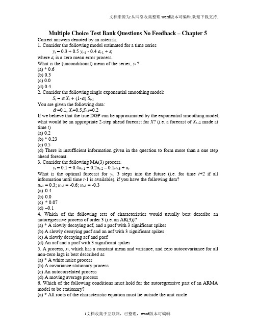
Multiple Choice Test Bank Questions No Feedback – Chapter 5 Correct answers denoted by an asterisk.1. Consider the following model estimated for a time seriesy t = 0.3 + 0.5 y t-1 - 0.4εt-1 +εtwhere εt is a zero mean error process.What is the (unconditional) mean of the series, y t ?(a) * 0.6(b) 0.3(c) 0.0(d) 0.42. Consider the following single exponential smoothing model:S t = α X t + (1-α) S t-1You are given the following data:αˆ=0.1, X t=0.5,S t-1=0.2If we believe that the true DGP can be approximated by the exponential smoothing model, what would be an appropriate 2-step ahead forecast for X? (i.e. a forecast of X t+2 made at time t)(a) 0.2(b) * 0.23(c) 0.5(d) There is insufficient information given in the question to form more than a one step ahead forecast.3. Consider the following MA(3) process.y t = 0.1 + 0.4u t-1 + 0.2u t-2– 0.1u t-3 + u tWhat is the optimal forecast for y t, 3 steps into the future (i.e. for time t+2 if all information until time t-1 is available), if you have the following data?u t-1 = 0.3; u t-2 = -0.6; u t-3 = -0.3(a)0.4(b)0.0(c)* 0.07(d)–0.14. Which of the following sets of characteristics would usually best describe an autoregressive process of order 3 (i.e. an AR(3))?(a) * A slowly decaying acf, and a pacf with 3 significant spikes(b) A slowly decaying pacf and an acf with 3 significant spikes(c) A slowly decaying acf and pacf(d) An acf and a pacf with 3 significant spikes5. A process, x t, which has a constant mean and variance, and zero autocovariance for all non-zero lags is best described as(a) * A white noise process(b) A covariance stationary process(c) An autocorrelated process(d) A moving average process6. Which of the following conditions must hold for the autoregressive part of an ARMA model to be stationary?(a) * All roots of the characteristic equation must lie outside the unit circle(b) All roots of the characteristic equation must lie inside the unit circle(c) All roots must be smaller than unity(d) At least one of the roots must be bigger than one in absolute value.7. Which of the following statements are true concerning time-series forecasting?(i) All time-series forecasting methods are essentially extrapolative.(ii) Forecasting models are prone to perform poorly following a structural break in a series.(iii) Forecasting accuracy often declines with prediction horizon.(iv) The mean squared errors of forecasts are usually very highly correlated with the profitability of employing those forecasts in a trading strategy.(a) (i), (ii), (iii), and (iv)(b) * (i), (ii) and (iii) only(c) (ii), (iii) only(d) (ii) and (iv) only8. If a series, y t, follows a random walk (with no drift), what is the optimal 1-step ahead forecast for y?(a)* The current value of y.(b)Zero.(c)The historical unweighted average of y.(d)An exponentially weighted average of previous values of y.9. Consider a series that follows an MA(1) with zero mean and a moving average coefficient of 0.4. What is the value of the autocorrelation function at lag 1?(a)0.4(b)1(c)*0.34(d)It is not possible to determine the value of the autocovariances without knowing thedisturbance variance.10. Which of the following statements are true?(i)An MA(q) can be expressed as an AR(infinity) if it is invertible(ii)An AR(p) can be written as an MA(infinity) if it is stationary(iii)The (unconditional) mean of an ARMA process will depend only on the intercept and on the AR coefficients and not on the MA coefficients(iv) A random walk series will have zero pacf except at lag 1(a)(ii) and (iv) only(b)(i) and (iii) only(c)(i), (ii), and (iii) only(d)* (i), (ii), (iii), and (iv).11. Consider the following picture and suggest the model from the following list that best characterises the process:(a)An AR(1)(b)An AR(2)(c)* An ARMA(1,1)(d)An MA(3)The acf is clearly declining very slowly in this case, which is consistent with their being an autoregressive part to the appropriate model. The pacf is clearly significant for lags one and two, but the question is does it them become insignificant for lags 2 and 4,indicating an AR(2) process, or does it remain significant, which would be more consistent with a mixed ARMA process? Well, given the huge size of the sample that gave rise to this acf and pacf, even a pacf value of 0.001 would still be statistically significant. Thus an ARMA process is the most likely candidate, although note that it would not be possible to tell from the acf and pacf which model from the ARMA family was more appropriate. The DGP for the data that generated this plot was y_t = 0.9 y_(t-1) – 0.3 u_(t-1) + u_t.12. Which of the following models can be estimated using ordinary least squares?(i)An AR(1)(ii) An ARMA(2,0)(iii) An MA(1)(iv) An ARMA(1,1)(a)(i) only(b)* (i) and (ii) only(c)(i), (ii), and (iii) only(d)(i), (ii), (iii), and (iv).13. If a series, y, is described as “mea n-reverting”, which model from the following list is likely to produce the best long-term forecasts for that series y?(a)A random walk(b)* The long term mean of the series(c)A model from the ARMA family(d)A random walk with drift14. Consider the following AR(2) model. What is the optimal 2-step ahead forecast for y if all information available is up to and including time t, if the values of y at time t, t-1 and t-2 are –0.3, 0.4 and –0.1 respectively, and the value of u at time t-1 is 0.3?y t = -0.1 + 0.75y t-1 - 0.125y t-2 + u t(a)-0.1(b)0.27(c)* -0.34(d)0.3015. What is the optimal three-step ahead forecast from the AR(2) model given in question 14?(a)-0.1(b)0.27(c)-0.34(d)* -0.3116. Suppose you had to guess at the most likely value of a one hundred step-ahead forecast for the AR(2) model given in question 14 – what would your forecast be?(a)-0.1(b)0.7(c)* –0.27(d)0.75。
高考英语《语法填空+阅读理解+应用文写作》真题含答案
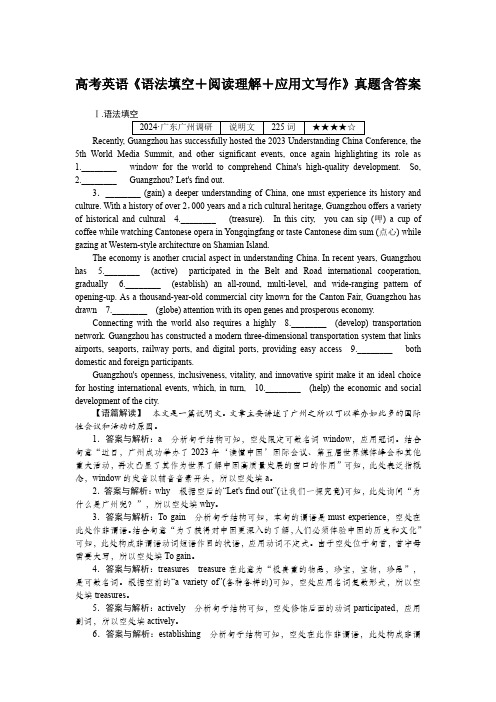
高考英语《语法填空+阅读理解+应用文写作》真题含答案Ⅰ.语法填空5th World Media Summit, and other significant events, once again highlighting its role as1.________ window for the world to comprehend China's highquality development. So,2.________ Guangzhou? Let's find out.3.________ (gain) a deeper understanding of China, one must experience its history and culture. With a history of over 2,000 years and a rich cultural heritage, Guangzhou offers a variety of historical and cultural 4.________ (treasure). In this city, you can sip (呷) a cup of coffee while watching Cantonese opera in Yongqingfang or taste Cantonese dim sum (点心) while gazing at Westernstyle architecture on Shamian Island.The economy is another crucial aspect in understanding China. In recent years, Guangzhou has 5.________ (active) participated in the Belt and Road international cooperation, gradually 6.________ (establish) an allround, multilevel, and wideranging pattern of openingup. As a thousandyearold commercial city known for the Canton Fair, Guangzhou has drawn 7.________ (globe) attention with its open genes and prosperous economy.Connecting with the world also requires a highly 8.________ (develop) transportation network. Guangzhou has constructed a modern threedimensional transportation system that links airports, seaports, railway ports, and digital ports, providing easy access 9.________ both domestic and foreign participants.Guangzhou's openness, inclusiveness, vitality, and innovative spirit make it an ideal choice for hosting international events, which, in turn, 10.________ (help) the economic and social development of the city.【语篇解读】本文是一篇说明文。
Forecasting

ForecastingWhy forecast?Features Common to all Forecasts∙Conditions in the past will continue in the future∙Rarely perfect∙Forecasts for groups tend to be more accurate than forecasts for individuals ∙Forecast accuracy declines as time horizon increasesElements of a Good Forecast∙Timely∙Accurate∙Reliable (should work consistently)∙Forecast expressed in meaningful units∙Communicated in writing∙Simple to understand and useSteps in Forecasting Process∙Determine purpose of the forecast∙Establish a time horizon∙Select forecasting technique∙Gather and analyze the appropriate data∙Prepare the forecast∙Monitor the forecastTypes of Forecasts∙Qualitativeo Judgment and opiniono Sales forceo Consumer surveyso Delphi technique∙Quantitativeo Regression and Correlation (associative)o Time seriesForecasts Based on Time Series Data∙What is Time Series?∙Components (behavior) of Time Series datao Trendo Cycleo Seasonalo Irregularo Random variationsNaïve MethodsNaïve Forecast – uses a single previous value of a time series as the basis of a forecast.Techniques for Averaging∙What is the purpose of averaging?∙Common Averaging Techniqueso Moving Averageso Exponential smoothingMoving AverageExponential SmoothingTechniques for TrendLinear Trend Equationline the of slope at of value pe riod time for fore cast from pe riods time of numbe r spe cifie d =====b ty a ty t t where t t 0:Curvilinear Trend Equationline the of slope at of value pe riod time for fore cast from pe riods time of numbe r spe cifie d =====b ty a ty t t where t t 0:Techniques for Seasonality∙ What is seasonality?∙ What are seasonal relatives or indexes?∙ How seasonal indexes are used:o Deseasonalizing datao Seasonalizing data∙ How indexes are computed (see Example 7 on page 109)Accuracy and Control of ForecastsMeasures of Accuracyo Mean Absolute Deviation (MAD)o Mean Squared Error (MSE)o Mean Absolute Percentage Error (MAPE) Forecast Control Measureo Tracking SignalMean Absolute Deviation (MAD)Mean Squared Error (or Deviation) (MSE)Mean Square Percentage Error (MAPE)Tracking SignalProblems:2 – Plot, Linear, MA, exponential Smoothing5 – Applying a linear trend to forecast15 – Computing seasonal relatives17 – Using indexes to deseasonalize values26 – Using MAD, MSE to measure forecast accuracyProblem 2 (110)National Mixer Inc., sells can openers. Monthly sales for a seven-month period were as follows:(a) Plot the monthly data on a sheet of graph paper.(b) Forecast September sales volume using each of the following:(1) A linear trend equation(2) A five-month moving average(3) Exponential smoothing with a smoothing constant equal to 0.20, assuming March forecast of19(000)(4) The Naïve Approach(5) A weighted average using 0.60 for August, 0.30 for July, and 0.10 for June(c) Which method seems least appropriate? Why?(d) What does use of the term sales rather than demand presume?EXCEL SOLUTION(a) Plot of the monthly dataHow to superimpose a trend line on the graph∙Click on the graph created above (note that when you do this an item called CHART will appear on the Excel menu bar)∙Click on Chart > Add Trend Line∙Click on the most appropriate Trend Regression Type∙Click OK(b) Forecast September sales volume using:(1) Linear Trend Equation∙Create a column for time period (t) codes (see column B)∙Click Tools > Data Analysis > Regression∙Fill in the appropriate information in the boxes in the Regression box that appearsCoded time periodSales dataCoded time period(2) Five-month moving average(3) Exponential Smoothing with a smoothing constant of 0.20, assuming March forecast of 19(000)∙Enter the smoothing factor in D1∙Enter “19” in D5 as forecast for March∙Create the exponential smoothing formula in D6, then copy it onto D7 to D11(4) The Naïve Approach(5) A weighted average using 0.60 for August, 0.30 for July, and 0.10 for JuneProblem 5 (110)A cosmetics manufactur er’s marketing department has developed a linear trend equation that can be used to predict annual sales of its popular Hand & Foot Cream.y t =80 + 15 twhere: y t = Annual sales (000 bottles) t0 = 1990(a) Are the annual sales increasing or decreasing? By how much?(b) Predict annual sales for the year 2006 using the equationProblem 15 (113)Obtain estimates of daily relatives for the number of customers at a restaurant for the evening meal, given the following data. (Hint: Use a seven-day moving average)Excel Solution∙Type a 7-day average formula in E6 ( =average(C3:c9) )∙In F6, type the formula =C6/E6∙Copy the formulas in E6 and F6 onto cells E7 to E27∙Compute the average ratio for Day 1 (see formula in E12)∙Copy and paste the formula in E12 onto E13 to E18 to complete the indexes for Days 2 to 7Problem 17 (113) – Using indexes to deseasonalize valuesNew car sales for a dealer in Cook County, Illinois, for the past year are shown in the following table, along with monthly (seasonal) relatives, which are supplied to the dealer by the regional distributor.(a) Plot the data. Does there seem to be a trend?(b) Deseasonalize car sales(c) Plot the deseasonalized data on the same graph as the original data. Comment on the two graphs.Excel Solution(a) Plot of original data (seasonalized car sales)(b) Deseasonalized Car Sales(c) Graph of seasonalized car sales versus deseasonalized car salesProblem 26 (115) – Using MAD, MSE, and MAPE to measure forecast accuracyTwo different forecasting techniques (F1 and F2) were used to forecast demand for cases of bottled water. Actual demand and the two sets of forecasts are as follows:(a) Compute MAD for each set of forecasts. Given your results, which forecast appears to be the mostaccurate? Explain.(b) Compute MSE for each set of forecasts. Given your results, which forecast appears to be the mostaccurate? Explain.(c) In practice, either MAD or MSE would be employed to compute forecast errors. What factors might leadyou to choose one rather than the other?(d) Compute MAPE for each data set. Which forecast appears to be more accurate?Excel Solution。
Sale Forecasting
Forecasting options
Executive opinion ------A convenient and inexpensive way to forecast. ------not a scientific technique. Sale force composite ------the sale representatives is the person most familiar with the local market area,especiallly competitive activity (the best position to predict local behavior) ------render subjective predictions and forecasting from a perspective that is too limited.
Forecasting options
Survey of customers ----this method is best for established product. ----For a new product concept ,customers’expections may not adequately indicate their actual behavior. Analysis of market factors ----is used when there is an association between sales and another varible ,called a factor. (For example , new housing starts may be a factor that predicts lumber sales.)
Forecasting
Business Forecaห้องสมุดไป่ตู้ting
The second possibility, management services, suffers from some of the problems of the data processing unit in being remote from the decision taking. Yet when the forecasts are for strategic decisions at board level this solution can be successful.
Business Forecasting
Forecasting is the process of using past events to make systematic predictions about future outcomes or trends. An observation popular with many forecasters is that “the only thing certain about a forecast is that it will be wrong.” Beneath the irony, this observation touches on an important point:
Business Forecasting
Introduction: Structure
The use of forecasting:
Managers must try to predict future conditions so that their goals and plans are realistic.
Time-Series Data AnalysisPPT教学课件
Exponential smoothing---a tool for noise filtering and forecasting
simple exponential smoothing--- the best
model for one-period-ahead forecasting
among 25 time series methods(Markridakis
et la )
2020/12/10
6
Statistical Methods- Exponential smoothing)
formula of the exponential smoothing:
Xt = b + t St = Xt + (1 - )St-1 Where
t: error b: constant
Time-Series Data Analysis
Statistical Methods Fuzzy Logic in Time-Series Data Analysis Chaos Theory in Time-Series Data Analysis Application of Artificial Neural Networks to Time-Series Data Analysis
Trend component --- a long-term change that does not repeat at the time range being considered Seasonal component(seasonality)--- regular fluctuations in systematic intervals. Noise (error)---irregular component
- 1、下载文档前请自行甄别文档内容的完整性,平台不提供额外的编辑、内容补充、找答案等附加服务。
- 2、"仅部分预览"的文档,不可在线预览部分如存在完整性等问题,可反馈申请退款(可完整预览的文档不适用该条件!)。
- 3、如文档侵犯您的权益,请联系客服反馈,我们会尽快为您处理(人工客服工作时间:9:00-18:30)。
25years of time series forecastingJan G.De Gooijer a,1,Rob J.Hyndman b ,*aDepartment of Quantitative Economics,University of Amsterdam,Roetersstraat 11,1018WB Amsterdam,The NetherlandsbDepartment of Econometrics and Business Statistics,Monash University,VIC 3800,AustraliaAbstractWe review the past 25years of research into time series forecasting.In this silver jubilee issue,we naturally highlight results published in journals managed by the International Institute of Forecasters (Journal of Forecasting 1982–1985and International Journal of Forecasting 1985–2005).During this period,over one third of all papers published in these journals concerned time series forecasting.We also review highly influential works on time series forecasting that have been published elsewhere during this period.Enormous progress has been made in many areas,but we find that there are a large number of topics in need of further development.We conclude with comments on possible future research directions in this field.D 2006International Institute of Forecasters.Published by Elsevier B.V .All rights reserved.Keywords:Accuracy measures;ARCH;ARIMA;Combining;Count data;Densities;Exponential smoothing;Kalman filter;Long memory;Multivariate;Neural nets;Nonlinearity;Prediction intervals;Regime-switching;Robustness;Seasonality;State space;Structural models;Transfer function;Univariate;V AR1.IntroductionThe International Institute of Forecasters (IIF)was established 25years ago and its silver jubilee provides an opportunity to review progress on time series forecasting.We highlight research published in journals sponsored by the Institute,although we also cover key publications in other journals.In 1982,the IIF set up the Journal of Forecasting (JoF ),publishedwith John Wiley and Sons.After a break with Wiley in 1985,2the IIF decided to start the International Journal of Forecasting (IJF ),published with Elsevier since 1985.This paper provides a selective guide to the literature on time series forecasting,covering the period 1982–2005and summarizing over 940papers including about 340papers published under the b IIF-flag Q .The proportion of papers that concern time series forecasting has been fairly stable over time.We also review key papers and books published else-where that have been highly influential to various developments in the field.The works referenced0169-2070/$-see front matter D 2006International Institute of Forecasters.Published by Elsevier B.V .All rights reserved.doi:10.1016/j.ijforecast.2006.01.001*Corresponding author.Tel.:+61399052358;fax:+61399055474.E-mail addresses: j.g.degooijer@uva.nl (J.G.De Gooijer),Rob.Hyndman@.au (R.J.Hyndman).1Tel.:+31205254244;fax:+31205254349.2The IIF was involved with JoF issue 44:1(1985).International Journal of Forecasting 22(2006)443–473/locate/ijforecastcomprise380journal papers and20books andmonographs.It was felt to be convenient to first classify thepapers according to the models(e.g.,exponentialsmoothing,ARIMA)introduced in the time seriesliterature,rather than putting papers under a headingassociated with a particular method.For instance,Bayesian methods in general can be applied to allmodels.Papers not concerning a particular modelwere then classified according to the various problems(e.g.,accuracy measures,combining)they address.Inonly a few cases was a subjective decision needed onour part to classify a paper under a particular sectionheading.To facilitate a quick overview in a particularfield,the papers are listed in alphabetical order undereach of the section headings.Determining what to include and what not toinclude in the list of references has been a problem.There may be papers that we have missed and papersthat are also referenced by other authors in this SilverAnniversary issue.As such the review is somewhatb selective Q,although this does not imply that a particular paper is unimportant if it is not reviewed.The review is not intended to be critical,but rathera(brief)historical and personal tour of the maindevelopments.Still,a cautious reader may detectcertain areas where the fruits of25years of intensiveresearch interest has been limited.Conversely,clearexplanations for many previously anomalous timeseries forecasting results have been provided by theend of2005.Section13discusses some currentresearch directions that hold promise for the future,but of course the list is far from exhaustive.2.Exponential smoothing2.1.PreambleTwenty-five years ago,exponential smoothingmethods were often considered a collection of adhoc techniques for extrapolating various types ofunivariate time series.Although exponential smooth-ing methods were widely used in business andindustry,they had received little attention fromstatisticians and did not have a well-developedstatistical foundation.These methods originated inthe1950s and1960s with the work of Brown(1959,1963),Holt(1957,reprinted2004),and Winters (1960).Pegels(1969)provided a simple but useful classification of the trend and the seasonal patterns depending on whether they are additive(linear)or multiplicative(nonlinear).Muth(1960)was the first to suggest a statistical foundation for simple exponential smoothing(SES) by demonstrating that it provided the optimal fore-casts for a random walk plus noise.Further steps towards putting exponential smoothing within a statistical framework were provided by Box and Jenkins(1970),Roberts(1982),and Abraham and Ledolter(1983,1986),who showed that some linear exponential smoothing forecasts arise as special cases of ARIMA models.However,these results did not extend to any nonlinear exponential smoothing methods.Exponential smoothing methods received a boost from two papers published in1985,which laid the foundation for much of the subsequent work in this area.First,Gardner(1985)provided a thorough review and synthesis of work in exponential smooth-ing to that date and extended Pegels’classification to include damped trend.This paper brought together a lot of existing work which stimulated the use of these methods and prompted a substantial amount of additional ter in the same year,Snyder (1985)showed that SES could be considered as arising from an innovation state space model(i.e.,a model with a single source of error).Although this insight went largely unnoticed at the time,in recent years it has provided the basis for a large amount of work on state space models underlying exponential smoothing methods.Most of the work since1980has involved studying the empirical properties of the methods(e.g.,Barto-lomei&Sweet,1989;Makridakis&Hibon,1991), proposals for new methods of estimation or initiali-zation(Ledolter&Abraham,1984),evaluation of the forecasts(McClain,1988;Sweet&Wilson,1988),or has concerned statistical models that can be consid-ered to underly the methods(e.g.,McKenzie,1984). The damped multiplicative methods of Taylor(2003) provide the only genuinely new exponential smooth-ing methods over this period.There have,of course, been numerous studies applying exponential smooth-ing methods in various contexts including computer components(Gardner,1993),air passengers(Grubb&J.G.De Gooijer,R.J.Hyndman/International Journal of Forecasting22(2006)443–473 444Masa,2001),and production planning(Miller& Liberatore,1993).The Hyndman,Koehler,Snyder,and Grose(2002) taxonomy(extended by Taylor,2003)provides a helpful categorization for describing the various methods.Each method consists of one of five types of trend(none,additive,damped additive,multiplica-tive,and damped multiplicative)and one of three types of seasonality(none,additive,and multiplica-tive).Thus,there are15different methods,the best known of which are SES(no trend,no seasonality), Holt’s linear method(additive trend,no seasonality), Holt–Winters’additive method(additive trend,addi-tive seasonality),and Holt–Winters’multiplicative method(additive trend,multiplicative seasonality).2.2.VariationsNumerous variations on the original methods have been proposed.For example,Carreno and Madina-veitia(1990)and Williams and Miller(1999)pro-posed modifications to deal with discontinuities,and Rosas and Guerrero(1994)looked at exponential smoothing forecasts subject to one or more con-straints.There are also variations in how and when seasonal components should be wton (1998)argued for renormalization of the seasonal indices at each time period,as it removes bias in estimates of level and seasonal components.Slightly different normalization schemes were given by Roberts(1982)and McKenzie(1986).Archibald and Koehler(2003)developed new renormalization equations that are simpler to use and give the same point forecasts as the original methods.One useful variation,part way between SES and Holt’s method,is SES with drift.This is equivalent to Holt’s method with the trend parameter set to zero. Hyndman and Billah(2003)showed that this method was also equivalent to Assimakopoulos and Nikolo-poulos(2000)b Theta method Q when the drift param-eter is set to half the slope of a linear trend fitted to the data.The Theta method performed extremely well in the M3-competition,although why this particular choice of model and parameters is good has not yet been determined.There has been remarkably little work in developing multivariate versions of the exponential smoothing methods for forecasting.One notable exception is Pfeffermann and Allon(1989)who looked at Israeli tourism data.Multivariate SES is used for process control charts(e.g.,Pan,2005),where it is called b multivariate exponentially weighted moving averages Q, but here the focus is not on forecasting.2.3.State space modelsOrd,Koehler,and Snyder(1997)built on the work of Snyder(1985)by proposing a class of innovation state space models which can be considered as underlying some of the exponential smoothing meth-ods.Hyndman et al.(2002)and Taylor(2003) extended this to include all of the15exponential smoothing methods.In fact,Hyndman et al.(2002) proposed two state space models for each method, corresponding to the additive error and the multipli-cative error cases.These models are not unique and other related state space models for exponential smoothing methods are presented in Koehler,Snyder, and Ord(2001)and Chatfield,Koehler,Ord,and Snyder(2001).It has long been known that some ARIMA models give equivalent forecasts to the linear exponential smoothing methods.The significance of the recent work on innovation state space models is that the nonlinear exponential smoothing methods can also be derived from statistical models.2.4.Method selectionGardner and McKenzie(1988)provided some simple rules based on the variances of differenced time series for choosing an appropriate exponential smoothing method.Tashman and Kruk(1996)com-pared these rules with others proposed by Collopy and Armstrong(1992)and an approach based on the BIC. Hyndman et al.(2002)also proposed an information criterion approach,but using the underlying state space models.2.5.RobustnessThe remarkably good forecasting performance of exponential smoothing methods has been addressed by several authors.Satchell and Timmermann(1995) and Chatfield et al.(2001)showed that SES is optimal for a wide range of data generating processes.In a small simulation study,Hyndman(2001)showed thatJ.G.De Gooijer,R.J.Hyndman/International Journal of Forecasting22(2006)443–473445simple exponential smoothing performed better than first order ARIMA models because it is not so subject to model selection problems,particularly when data are non-normal.2.6.Prediction intervalsOne of the criticisms of exponential smoothing methods25years ago was that there was no way to produce prediction intervals for the forecasts.The first analytical approach to this problem was to assume that the series were generated by deterministic functions of time plus white noise(Brown,1963;Gardner,1985; McKenzie,1986;Sweet,1985).If this was so,a regression model should be used rather than expo-nential smoothing methods;thus,Newbold and Bos (1989)strongly criticized all approaches based on this assumption.Other authors sought to obtain prediction intervals via the equivalence between exponential smoothing methods and statistical models.Johnston and Harrison (1986)found forecast variances for the simple and Holt exponential smoothing methods for state space models with multiple sources of errors.Yar and Chatfield(1990)obtained prediction intervals for the additive Holt–Winters’method by deriving the underlying equivalent ARIMA model.Approximate prediction intervals for the multiplicative Holt–Win-ters’method were discussed by Chatfield and Yar (1991),making the assumption that the one-step-ahead forecast errors are independent.Koehler et al. (2001)also derived an approximate formula for the forecast variance for the multiplicative Holt–Winters’method,differing from Chatfield and Yar(1991)only in how the standard deviation of the one-step-ahead forecast error is estimated.Ord et al.(1997)and Hyndman et al.(2002)used the underlying innovation state space model to simulate future sample paths,and thereby obtained prediction intervals for all the exponential smoothing methods.Hyndman,Koehler,Ord,and Snyder (2005)used state space models to derive analytical prediction intervals for15of the30methods, including all the commonly used methods.They provide the most comprehensive algebraic approach to date for handling the prediction distribution problem for the majority of exponential smoothing methods.2.7.Parameter space and model propertiesIt is common practice to restrict the smoothing parameters to the range0to1.However,now that underlying statistical models are available,the natural (invertible)parameter space for the models can be used instead.Archibald(1990)showed that it is possible for smoothing parameters within the usual intervals to produce non-invertible models.Conse-quently,when forecasting,the impact of change in the past values of the series is non-negligible.Intuitively, such parameters produce poor forecasts and the forecast performance wton(1998)also discussed this problem.3.ARIMA models3.1.PreambleEarly attempts to study time series,particularly in the19th century,were generally characterized by the idea of a deterministic world.It was the major contribution of Yule(1927)which launched the notion of stochasticity in time series by postulating that every time series can be regarded as the realization of a stochastic process.Based on this simple idea,a number of time series methods have been developed since then.Workers such as Slutsky,Walker,Yaglom, and Yule first formulated the concept of autoregres-sive(AR)and moving average(MA)models.Wold’s decomposition theorem led to the formulation and solution of the linear forecasting problem of Kolmo-gorov(1941).Since then,a considerable body of literature has appeared in the area of time series, dealing with parameter estimation,identification, model checking,and forecasting;see,e.g.,Newbold (1983)for an early survey.The publication Time Series Analysis:Forecasting and Control by Box and Jenkins(1970)3integrated the existing knowledge.Moreover,these authors developed a coherent,versatile three-stage iterative3The book by Box,Jenkins,and Reinsel(1994)with Gregory Reinsel as a new co-author is an updated version of the b classic Q Box and Jenkins(1970)text.It includes new material on intervention analysis,outlier detection,testing for unit roots,and process control.J.G.De Gooijer,R.J.Hyndman/International Journal of Forecasting22(2006)443–473 446cycle for time series identification,estimation,and verification(rightly known as the Box–Jenkins approach).The book has had an enormous impact on the theory and practice of modern time series analysis and forecasting.With the advent of the computer,it popularized the use of autoregressive integrated moving average(ARIMA)models and their extensions in many areas of science.Indeed,forecast-ing discrete time series processes through univariate ARIMA models,transfer function(dynamic regres-sion)models,and multivariate(vector)ARIMA models has generated quite a few IJF papers.Often these studies were of an empirical nature,using one or more benchmark methods/models as a comparison. Without pretending to be complete,Table1gives a list of these studies.Naturally,some of these studies are more successful than others.In all cases,the forecasting experiences reported are valuable.They have also been the key to new developments,which may be summarized as follows.3.2.UnivariateThe success of the Box–Jenkins methodology is founded on the fact that the various models can, between them,mimic the behaviour of diverse types of series—and do so adequately without usually requiring very many parameters to be estimated in the final choice of the model.However,in the mid-sixties,the selection of a model was very much a matter of the researcher’s judgment;there was no algorithm to specify a model uniquely.Since then,Table1A list of examples of real applicationsDataset Forecast horizon Benchmark ReferenceUnivariate ARIMAElectricity load(min)1–30min Wiener filter Di Caprio,Genesio,Pozzi,and Vicino(1983)Quarterly automobile insurancepaid claim costs8quarters Log-linear regression Cummins and Griepentrog(1985)Daily federal funds rate1day Random walk Hein and Spudeck(1988)Quarterly macroeconomic data1–8quarters Wharton model Dhrymes and Peristiani(1988) Monthly department store sales1month Simple exponential smoothing Geurts and Kelly(1986,1990),Pack(1990)Monthly demand for telephone services3years Univariate state space Grambsch and Stahel(1990)Yearly population totals20–30years Demographic models Pflaumer(1992)Monthly tourism demand1–24months Univariate state space,multivariate state spacedu Preez and Witt(2003)Dynamic regression/transfer functionMonthly telecommunications traffic1month Univariate ARIMA Layton,Defris,and Zehnwirth(1986) Weekly sales data2years n.a.Leone(1987)Daily call volumes1week Holt–Winters Bianchi,Jarrett,and Hanumara(1998) Monthly employment levels1–12months Univariate ARIMA Weller(1989)Monthly and quarterly consumptionof natural gas1month/1quarter Univariate ARIMA Liu and Lin(1991)Monthly electricity consumption1–3years Univariate ARIMA Harris and Liu(1993)VARIMAYearly municipal budget data Yearly(in-sample)Univariate ARIMA Downs and Rocke(1983)Monthly accounting data1month Regression,univariate,ARIMA,transfer functionHillmer,Larcker,and Schroeder(1983)Quarterly macroeconomic data1–10quarters Judgmental methods,univariateARIMAO¨ller(1985)Monthly truck sales1–13months Univariate ARIMA,Holt–Winters Heuts and Bronckers(1988)Monthly hospital patient movements2years Univariate ARIMA,Holt–Winters Lin(1989)Quarterly unemployment rate1–8quarters Transfer function Edlund and Karlsson(1993)J.G.De Gooijer,R.J.Hyndman/International Journal of Forecasting22(2006)443–473447many techniques and methods have been suggested to add mathematical rigour to the search process of an ARMA model,including Akaike’s information crite-rion(AIC),Akaike’s final prediction error(FPE),and the Bayes information criterion(BIC).Often these criteria come down to minimizing(in-sample)one-step-ahead forecast errors,with a penalty term for overfitting.FPE has also been generalized for multi-step-ahead forecasting(see, e.g.,Bhansali,1996, 1999),but this generalization has not been utilized by applied workers.This also seems to be the case with criteria based on cross-validation and split-sample validation(see,e.g.,West,1996)principles, making use of genuine out-of-sample forecast errors; see Pen˜a and Sa´nchez(2005)for a related approach worth considering.There are a number of methods(cf.Box et al., 1994)for estimating the parameters of an ARMA model.Although these methods are equivalent asymptotically,in the sense that estimates tend to the same normal distribution,there are large differ-ences in finite sample properties.In a comparative study of software packages,Newbold,Agiakloglou, and Miller(1994)showed that this difference can be quite substantial and,as a consequence,may influ-ence forecasts.They recommended the use of full maximum likelihood.The effect of parameter esti-mation errors on the probability limits of the forecasts was also noticed by Zellner(1971).He used a Bayesian analysis and derived the predictive distri-bution of future observations by treating the param-eters in the ARMA model as random variables.More recently,Kim(2003)considered parameter estimation and forecasting of AR models in small samples.He found that(bootstrap)bias-corrected parameter esti-mators produce more accurate forecasts than the least squares ndsman and Damodaran(1989) presented evidence that the James-Stein ARIMA parameter estimator improves forecast accuracy relative to other methods,under an MSE loss criterion.If a time series is known to follow a univariate ARIMA model,forecasts using disaggregated obser-vations are,in terms of MSE,at least as good as forecasts using aggregated observations.However,in practical applications,there are other factors to be considered,such as missing values in disaggregated series.Both Ledolter(1989)and Hotta(1993)analyzed the effect of an additive outlier on theforecast intervals when the ARIMA model parametersare estimated.When the model is stationary,Hotta andCardoso Neto(1993)showed that the loss ofefficiency using aggregated data is not large,even ifthe model is not known.Thus,prediction could bedone by either disaggregated or aggregated models.The problem of incorporating external(prior)information in the univariate ARIMA forecasts hasbeen considered by Cholette(1982),Guerrero(1991),and de Alba(1993).As an alternative to the univariate ARIMAmethodology,Parzen(1982)proposed the ARARMAmethodology.The key idea is that a time series istransformed from a long-memory AR filter to a short-memory filter,thus avoiding the b harsher Q differenc-ing operator.In addition,a different approach to thed conventional T Box–Jenkins identification step is used.In the M-competition(Makridakis et al.,1982),the ARARMA models achieved the lowestMAPE for longer forecast horizons.Hence,it issurprising to find that,apart from the paper by Meadeand Smith(1985),the ARARMA methodology hasnot really taken off in applied work.Its ultimate valuemay perhaps be better judged by assessing the studyby Meade(2000)who compared the forecastingperformance of an automated and non-automatedARARMA method.Automatic univariate ARIMA modelling has beenshown to produce one-step-ahead forecasts as accu-rate as those produced by competent modellers(Hill&Fildes,1984;Libert,1984;Poulos,Kvanli,&Pavur,1987;Texter&Ord,1989).Several softwarevendors have implemented automated time seriesforecasting methods(including multivariate methods);see,e.g.,Geriner and Ord(1991),Tashman and Leach(1991),and Tashman(2000).Often these methods actas black boxes.The technology of expert systems(Me´lard&Pasteels,2000)can be used to avoid thisproblem.Some guidelines on the choice of anautomatic forecasting method are provided by Chat-field(1988).Rather than adopting a single AR model for allforecast horizons,Kang(2003)empirically investi-gated the case of using a multi-step-ahead forecastingAR model selected separately for each horizon.Theforecasting performance of the multi-step-ahead pro-cedure appears to depend on,among other things,J.G.De Gooijer,R.J.Hyndman/International Journal of Forecasting22(2006)443–473 448optimal order selection criteria,forecast periods, forecast horizons,and the time series to be forecast.3.3.Transfer functionThe identification of transfer function models can be difficult when there is more than one input variable.Edlund(1984)presented a two-step method for identification of the impulse response function when a number of different input variables are correlated.Koreisha(1983)established various rela-tionships between transfer functions,causal implica-tions,and econometric model specification.Gupta (1987)identified the major pitfalls in causality testing. Using principal component analysis,a parsimonious representation of a transfer function model was suggested by del Moral and Valderrama(1997). Krishnamurthi,Narayan,and Raj(1989)showed how more accurate estimates of the impact of interventions in transfer function models can be obtained by using a control variable.3.4.MultivariateThe vector ARIMA(VARIMA)model is a multivariate generalization of the univariate ARIMA model.The population characteristics of V ARMA processes appear to have been first derived by Quenouille(1957),although software to implement them only became available in the1980s and1990s. Since V ARIMA models can accommodate assump-tions on exogeneity and on contemporaneous relation-ships,they offered new challenges to forecasters and policymakers.Riise and Tjøstheim(1984)addressed the effect of parameter estimation on VARMA forecasts.Cholette and Lamy(1986)showed how smoothing filters can be built into V ARMA models. The smoothing prevents irregular fluctuations in explanatory time series from migrating to the forecasts of the dependent series.To determine the maximum forecast horizon of V ARMA processes,De Gooijer and Klein(1991)established the theoretical properties of cumulated multi-step-ahead forecasts and cumulat-ed multi-step-ahead forecast errors.Lu¨tkepohl(1986) studied the effects of temporal aggregation and systematic sampling on forecasting,assuming that the disaggregated(stationary)variable follows a V ARMA process with unknown ter,Bidar-kota(1998)considered the same problem but with the observed variables integrated rather than stationary.Vector autoregressions(VARs)constitute a special case of the more general class of V ARMA models.In essence,a VAR model is a fairly unrestricted (flexible)approximation to the reduced form of a wide variety of dynamic econometric models.V AR models can be specified in a number of ways.Funke (1990)presented five different V AR specifications and compared their forecasting performance using monthly industrial production series.Dhrymes and Thomakos(1998)discussed issues regarding the identification of structural V ARs.Hafer and Sheehan (1989)showed the effect on V AR forecasts of changes in the model structure.Explicit expressions for V AR forecasts in levels are provided by Arin˜o and Franses (2000);see also Wieringa and Horva´th(2005). Hansson,Jansson,and Lo¨f(2005)used a dynamic factor model as a starting point to obtain forecasts from parsimoniously parametrized V ARs.In general,VAR models tend to suffer from d overfitting T with too many free insignificant param-eters.As a result,these models can provide poor out-of-sample forecasts,even though within-sample fit-ting is good;see,e.g.,Liu,Gerlow,and Irwin(1994) and Simkins(1995).Instead of restricting some of the parameters in the usual way,Litterman(1986)and others imposed a prior distribution on the parameters, expressing the belief that many economic variables behave like a random walk.BV AR models have been chiefly used for macroeconomic forecasting(Artis& Zhang,1990;Ashley,1988;Holden&Broomhead, 1990;Kunst&Neusser,1986),for forecasting market shares(Ribeiro Ramos,2003),for labor market forecasting(LeSage&Magura,1991),for business forecasting(Spencer,1993),or for local economic forecasting(LeSage,1989).Kling and Bessler(1985) compared out-of-sample forecasts of several then-known multivariate time series methods,including Litterman’s BV AR model.The Engle and Granger(1987)concept of cointe-gration has raised various interesting questions re-garding the forecasting ability of error correction models(ECMs)over unrestricted V ARs and BV ARs. Shoesmith(1992),Shoesmith(1995),Tegene and Kuchler(1994),and Wang and Bessler(2004) provided empirical evidence to suggest that ECMs outperform V ARs in levels,particularly over longerJ.G.De Gooijer,R.J.Hyndman/International Journal of Forecasting22(2006)443–473449。
