Chapter 6 Solutions
医学英语Chapter 6_Obesity Causes and Prevention

《当代医学·英语综合教程 II—关注健康》
catastrophic a. 悲惨的,灾难的
wage v.
开展,进行
adaptive a. 适应的,适合的
prescriptive a. 规定的,惯例的
gastric a. 胃的
bypass n. 旁路
morbid a. 病态的
obese a.
过度肥胖的
Obesity and Social Ties
《当代医学·英语综合教程 II—关注健康》
Chapter 6
When one person gains weight, their close friends often follow. Researchers have just (1)_o_f_f_e_re_d__ evidence in a study that says obesity appears to (2) _s_p_re_a_d__ through social ties. But the findings might also offer hope.
lipid n.
类脂(化合)物
execute v.
实施,执行
havoc n.
大破坏,浩劫
undernourished a. 营养不足的
《当代医学·英语综合教程 II—关注健康》
Chapter 6
strategically ad. exertion n. sedentary a. winch n. casket n.
《当代医学·英语综合教程 II—关注健康》
Chapter 6
obese. A sister or brother of a person who became obese had a 40 percent increased chance of becoming obese. The (10) _ri_s_k___ for a wife or husband was a little less than that.
数据库系统基础教程第六章答案

Solutions Chapter 6Attributes must be separated by commas. Thus here B is an alias of A.6.1.2a)SELECT address AS Studio_AddressFROM StudioWHERE NAME = 'MGM';b)SELECT birthdate AS Star_BirthdateFROM MovieStarWHERE name = 'Sandra Bullock';c)SELECT starNameFROM StarsInWHERE movieYear = 1980OR movieTitle LIKE '%Love%';However, above query will also return words that have the substring Love e.g. Lover. Below query will only return movies that have title containing the word Love.SELECT starNameFROM StarsInWHERE movieYear = 1980OR movieTitle LIKE 'Love %'OR movieTitle LIKE '% Love %'OR movieTitle LIKE '% Love'OR movieTitle = 'Love';d)SELECT name AS Exec_NameFROM MovieExecWHERE netWorth >= 10000000;e)SELECT name AS Star_NameFROM movieStarWHERE gender = 'M'OR address LIKE '% Malibu %';a)SELECT model,speed,hdFROM PCWHERE price < 1000 ;MODEL SPEED HD----- ---------- ------1002 2.10 2501003 1.42 801004 2.80 2501005 3.20 2501007 2.20 2001008 2.20 2501009 2.00 2501010 2.80 3001011 1.86 1601012 2.80 1601013 3.06 8011 record(s) selected.b)SELECT model ,speed AS gigahertz,hd AS gigabytesFROM PCWHERE price < 1000 ;MODEL GIGAHERTZ GIGABYTES ----- ---------- ---------1002 2.10 2501003 1.42 801004 2.80 2501005 3.20 2501007 2.20 2001008 2.20 2501009 2.00 2501010 2.80 3001011 1.86 1601012 2.80 1601013 3.06 8011 record(s) selected.c)SELECT makerFROM ProductWHERE TYPE = 'printer' ; MAKER-----DDEEEHH7 record(s) selected.d)SELECT model,ram ,screenFROM LaptopWHERE price > 1500 ; MODEL RAM SCREEN ----- ------ -------2001 2048 20.12005 1024 17.02006 2048 15.42010 2048 15.44 record(s) selected.e)SELECT *FROM PrinterWHERE color ;MODEL CASE TYPE PRICE----- ----- -------- ------3001 TRUE ink-jet 993003 TRUE laser 9993004 TRUE ink-jet 1203006 TRUE ink-jet 1003007 TRUE laser 2005 record(s) selected.Note: Implementation of Boolean type is optional in SQL standard (feature IDT031). PostgreSQL has implementation similar to above example. Other DBMS provide equivalent support. E.g. In DB2 the column type can be declare as SMALLINT with CONSTRAINT that the value can be 0 or 1. The result can be returned as Boolean type CHAR using CASE.CREATE TABLE Printer(model CHAR(4) UNIQUE NOT NULL,color SMALLINT ,type VARCHAR(8) ,price SMALLINT ,CONSTRAINT Printer_ISCOLOR CHECK(color IN(0,1)));SELECT model,CASE colorWHEN 1THEN 'TRUE'WHEN 0THEN 'FALSE'ELSE 'ERROR'END CASE ,type,priceFROM PrinterWHERE color = 1;f)SELECT model,hdFROM PCWHERE speed = 3.2AND price < 2000;MODEL HD----- ------1005 2501006 3202 record(s) selected.6.1.4a)SELECT class,countryFROM ClassesWHERE numGuns >= 10 ; CLASS COUNTRY------------------ ------------ Tennessee USA1 record(s) selected.b)SELECT name AS shipName FROM ShipsWHERE launched < 1918 ; SHIPNAME------------------HarunaHieiKirishimaKongoRamilliesRenownRepulseResolutionRevengeRoyal OakRoyal Sovereign11 record(s) selected.c)SELECT ship AS shipName, battleFROM OutcomesWHERE result = 'sunk' ; SHIPNAME BATTLE------------------ ------------------ Arizona Pearl Harbor Bismark Denmark Strait Fuso Surigao Strait Hood Denmark Strait Kirishima Guadalcanal Scharnhorst North Cape Yamashiro Surigao Strait 7 record(s) selected.d)SELECT name AS shipNameFROM ShipsWHERE name = class ;SHIPNAME------------------IowaKongoNorth CarolinaRenownRevengeYamato6 record(s) selected.e)SELECT name AS shipNameFROM ShipsWHERE name LIKE 'R%';SHIPNAME------------------RamilliesRenownRepulseResolutionRevengeRoyal OakRoyal Sovereign7 record(s) selected.Note: As mentioned in exercise 2.4.3, there are some dangling pointers and to retrieve all ships a UNION of Ships and Outcomes is required.Below query returns 8 rows including ship named Rodney.SELECT name AS shipNameFROM ShipsWHERE name LIKE 'R%'UNIONSELECT ship AS shipNameFROM OutcomesWHERE ship LIKE 'R%';f) Only using a filter like '% % %' will incorrectly match name such as ' a b ' since % can match any sequence of 0 or more characters.SELECT name AS shipNameFROM ShipsWHERE name LIKE '_% _% _%' ;SHIPNAME------------------0 record(s) selected.Note: As in (e), UNION with results from Outcomes.SELECT name AS shipNameFROM ShipsWHERE name LIKE '_% _% _%'UNIONSELECT ship AS shipNameFROM OutcomesWHERE ship LIKE '_% _% _%' ;SHIPNAME------------------Duke of YorkKing George VPrince of Wales3 record(s) selected.6.1.5a)The resulting expression is false when neither of (a=10) or (b=20) is TRUE.a = 10b = 20 a = 10 OR b = 20NULL TRUE TRUETRUE NULL TRUEFALSE TRUE TRUETRUE FALSE TRUETRUE TRUE TRUEb)The resulting expression is only TRUE when both (a=10) and (b=20) are TRUE.a = 10b = 20 a = 10 AND b = 20TRUE TRUE TRUEThe expression is always TRUE unless a is NULL.a < 10 a >= 10 a = 10 ANDb = 20TRUE FALSE TRUEFALSE TRUE TRUEd)The expression is TRUE when a=b except when the values are NULL.a b a = bNOT NULL NOT NULL TRUE when a=b; else FALSEe)Like in (d), the expression is TRUE when a<=b except when the values are NULL.a b a <= bNOT NULL NOT NULL TRUE when a<=b; else FALSE6.1.6SELECT *FROM MoviesWHERE LENGTH IS NOT NULL;6.2.1a)SELECT AS starNameFROM MovieStar M,StarsIn SWHERE = S.starNameAND S.movieTitle = 'Titanic'AND M.gender = 'M';b)SELECT S.starNameFROM Movies M ,StarsIn S,Studios TWHERE ='MGM'AND M.year = 1995AND M.title = S.movieTitleAND M.studioName = ;SELECT AS presidentName FROM MovieExec X,Studio TWHERE X.cert# = T.presC#AND = 'MGM';d)SELECT M1.titleFROM Movies M1,Movies M2WHERE M1.length > M2.lengthAND M2.title ='Gone With the Wind' ;e)SELECT AS execNameFROM MovieExec X1,MovieExec X2WHERE Worth > WorthAND = 'Merv Griffin' ;6.2.2a)SELECT R.maker AS manufacturer,L.speed AS gigahertzFROM Product R,Laptop LWHERE L.hd >= 30AND R.model = L.model ; MANUFACTURER GIGAHERTZ------------ ----------A 2.00A 2.16A 2.00B 1.83E 2.00E 1.73E 1.80F 1.60F 1.60G 2.0010 record(s) selected.SELECT R.model,P.priceFROM Product R,PC PWHERE R.maker = 'B'AND R.model = P.model UNIONSELECT R.model,L.priceFROM Product R,Laptop LWHERE R.maker = 'B'AND R.model = L.model UNIONSELECT R.model,T.priceFROM Product R,Printer TWHERE R.maker = 'B'AND R.model = T.model ; MODEL PRICE----- ------1004 6491005 6301006 10492007 14294 record(s) selected.c)SELECT R.makerFROM Product R,Laptop LWHERE R.model = L.model EXCEPTSELECT R.makerFROM Product R,PC PWHERE R.model = P.model ; MAKER-----FG2 record(s) selected.SELECT DISTINCT P1.hd FROM PC P1,PC P2WHERE P1.hd =P2.hdAND P1.model > P2.model ; Alternate Answer:SELECT DISTINCT P.hdFROM PC PGROUP BY P.hdHAVING COUNT(P.model) >= 2 ;e)SELECT P1.model,P2.modelFROM PC P1,PC P2WHERE P1.speed = P2.speed AND P1.ram = P2.ramAND P1.model < P2.model ; MODEL MODEL----- -----1004 10121 record(s) selected.f)SELECT M.makerFROM(SELECT maker,R.modelFROM PC P,Product RWHERE SPEED >= 3.0AND P.model=R.modelUNIONSELECT maker,R.modelFROM Laptop L,Product RWHERE speed >= 3.0AND L.model=R.model) MGROUP BY M.makerHAVING COUNT(M.model) >= 2 ; MAKER-----B1 record(s) selected.6.2.3a)SELECT FROM Ships S,Classes CWHERE S.class = C.classAND C.displacement > 35000;NAME------------------IowaMissouriMusashiNew JerseyNorth CarolinaWashingtonWisconsinYamato8 record(s) selected.b)SELECT ,C.displacement,C.numGunsFROM Ships S ,Outcomes O,Classes CWHERE = O.shipAND S.class = C.classAND O.battle = 'Guadalcanal' ;NAME DISPLACEMENT NUMGUNS------------------ ------------ -------Kirishima 32000 8Washington 37000 92 record(s) selected.Note:South Dakota was also engaged in battle of Guadalcanal but not chosen since it is not in Ships table(Hence, no information regarding it's Class isavailable).SELECT name shipName FROM ShipsUNIONSELECT ship shipName FROM Outcomes ; SHIPNAME------------------ArizonaBismarkCaliforniaDuke of YorkFusoHarunaHieiHoodIowaKing George VKirishimaKongoMissouriMusashiNew JerseyNorth CarolinaPrince of Wales RamilliesRenownRepulseResolutionRevengeRodneyRoyal OakRoyal Sovereign ScharnhorstSouth DakotaTenneseeTennesseeWashingtonWest VirginiaWisconsinYamashiroYamato34 record(s) selected.SELECT C1.countryFROM Classes C1,Classes C2WHERE C1.country = C2.country AND C1.type = 'bb'AND C2.type = 'bc' ; COUNTRY------------Gt. BritainJapan2 record(s) selected.e)SELECT O1.shipFROM Outcomes O1,Battles B1WHERE O1.battle = AND O1.result = 'damaged'AND EXISTS(SELECT B2.dateFROM Outcomes O2,Battles B2WHERE O2.battle= AND O1.ship = O2.shipAND B1.date < B2.date) ;SHIP------------------0 record(s) selected.f)SELECT O.battleFROM Outcomes O,Ships S ,Classes CWHERE O.ship = AND S.class = C.class GROUP BY C.country,O.battleHAVING COUNT(O.ship) > 3; SELECT O.battleFROM Ships S ,Classes C,Outcomes OWHERE C.Class = S.classAND O.ship = GROUP BY C.country,O.battleHAVING COUNT(O.ship) >= 3;6.2.4Since tuple variables are not guaranteed to be unique, every relation Ri should be renamed using an alias. Every tuple variable should be qualified with the alias. Tuple variables for repeating relations will also be distinctlyidentified this way.Thus the query will be likeSELECT A1.COLL1,A1.COLL2,A2.COLL1,…FROM R1 A1,R2 A2,…,Rn AnWH ERE A1.COLL1=A2.COLC2,…6.2.5Again, create a tuple variable for every Ri, i=1,2,...,nThat is, the FROM clause isFROM R1 A1, R2 A2,...,Rn An.Now, build the WHERE clause from C by replacing every reference to some attribute COL1 of Ri by Ai.COL1. In addition apply Natural Join i.e. add condition to check equality of common attribute names between Ri and Ri+1 for all i from 0 to n-1. Also, build the SELECT clause from list of attributes L by replacing every attribute COLj of Ri by Ai.COLj.6.3.1a)SELECT DISTINCT makerFROM ProductWHERE model IN(SELECT modelFROM PCWHERE speed >= 3.0);SELECT DISTINCT R.makerFROM Product RWHERE EXISTS(SELECT P.modelFROM PC PWHERE P.speed >= 3.0AND P.model =R.model);SELECT P1.modelFROM Printer P1WHERE P1.price >= ALL(SELECT P2.priceFROM Printer P2) ;SELECT P1.modelFROM Printer P1WHERE P1.price IN(SELECT MAX(P2.price)FROM Printer P2) ;c)SELECT L.modelFROM Laptop LWHERE L.speed < ANY(SELECT P.speedFROM PC P) ;SELECT L.modelFROM Laptop LWHERE EXISTS(SELECT P.speedFROM PC PWHERE P.speed >= L.speed ) ;SELECT modelFROM(SELECT model,priceFROM PCUNIONSELECT model,priceFROM LaptopUNIONSELECT model,priceFROM Printer) M1WHERE M1.price >= ALL (SELECT priceFROM PCUNIONSELECT priceFROM LaptopUNIONSELECT priceFROM Printer) ;(d) – contd --SELECT modelFROM(SELECT model,priceFROM PCUNIONSELECT model,priceFROM LaptopUNIONSELECT model,priceFROM Printer) M1WHERE M1.price IN(SELECT MAX(price)FROM(SELECT priceFROM PCUNIONSELECT priceFROM LaptopUNIONSELECT priceFROM Printer) M2) ;e)SELECT R.makerFROM Product R,Printer TWHERE R.model =T.model AND T.price <= ALL(SELECT MIN(price)FROM Printer);SELECT R.makerFROM Product R,Printer T1WHERE R.model =T1.model AND T1.price IN(SELECT MIN(T2.price) FROM Printer T2);f)SELECT R1.makerFROM Product R1,PC P1WHERE R1.model=P1.modelAND P1.ram IN(SELECT MIN(ram)FROM PC)AND P1.speed >= ALL(SELECT P1.speedFROM Product R1,PC P1WHERE R1.model=P1.model AND P1.ram IN(SELECT MIN(ram)FROM PC));SELECT R1.makerFROM Product R1,PC P1WHERE R1.model=P1.modelAND P1.ram =(SELECT MIN(ram)FROM PC)AND P1.speed IN(SELECT MAX(P1.speed)FROM Product R1,PC P1WHERE R1.model=P1.model AND P1.ram IN(SELECT MIN(ram)FROM PC));6.3.2a)SELECT C.countryFROM Classes CWHERE numGuns IN(SELECT MAX(numGuns)FROM Classes);SELECT C.countryFROM Classes CWHERE numGuns >= ALL(SELECT numGunsFROM Classes);b)SELECT DISTINCT C.class FROM Classes C,Ships SWHERE C.class = S.classAND EXISTS(SELECT shipFROM Outcomes OWHERE O.result='sunk' AND O.ship = ) ;SELECT DISTINCT C.class FROM Classes C,Ships SWHERE C.class = S.classAND IN(SELECT shipFROM Outcomes OWHERE O.result='sunk' ) ;c)SELECT FROM Ships SWHERE S.class IN(SELECT classFROM Classes CWHERE bore=16) ;SELECT FROM Ships SWHERE EXISTS(SELECT classFROM Classes CWHERE bore =16AND C.class = S.class );SELECT O.battleFROM Outcomes OWHERE O.ship IN(SELECT nameFROM Ships SWHERE S.Class ='Kongo' );SELECT O.battleFROM Outcomes OWHERE EXISTS(SELECT nameFROM Ships SWHERE S.Class ='Kongo' AND = O.ship );SELECT FROM Ships S,Classes CWHERE S.Class = C.ClassAND numGuns >= ALL(SELECT numGunsFROM Ships S2,Classes C2WHERE S2.Class = C2.Class AND C2.bore = C.bore) ;SELECT FROM Ships S,Classes CWHERE S.Class = C.ClassAND numGuns IN(SELECT MAX(numGuns)FROM Ships S2,Classes C2WHERE S2.Class = C2.Class AND C2.bore = C.bore) ;Better answer;SELECT FROM Ships S,Classes CWHERE S.Class = C.ClassAND numGuns >= ALL(SELECT numGunsFROM Classes C2WHERE C2.bore = C.bore) ;SELECT FROM Ships S,Classes CWHERE S.Class = C.ClassAND numGuns IN(SELECT MAX(numGuns)FROM Classes C2WHERE C2.bore = C.bore) ;6.3.3SELECT titleFROM MoviesGROUP BY titleHAVING COUNT(title) > 1 ;6.3.4SELECT FROM Ships S,Classes CWHERE S.Class = C.Class ;Assumption: In R1 join R2, the rows of R2 are unique on the joining columns. SELECT COLL12,COLL13,COLL14FROM R1WHERE COLL12 IN(SELECT COL22FROM R2)AND COLL13 IN(SELECT COL33FROM R3)AND COLL14 IN(SELECT COL44FROM R4) ...6.3.5(a)SELECT ,S.addressFROM MovieStar S,MovieExec EWHERE S.gender ='F'AND Worth > 10000000AND = AND S.address = E.address ;Note: As mentioned previously in the book, the names of stars are unique. However no such restriction exists for executives. Thus, both name and address are required as join columns.Alternate solution:SELECT name,addressFROM MovieStarWHERE gender = 'F'AND (name, address) IN(SELECT name,addressFROM MovieExecWHERE netWorth > 10000000) ;(b)SELECT name,addressFROM MovieStarWHERE (name,address) NOT IN(SELECT name addressFROM MovieExec) ;6.3.6By replacing the column in subquery with a constant and using IN subquery forthe constant, statement equivalent to EXISTS can be found.i.e. replace "WHERE EXISTS (SELECT C1 FROM R1..)" by "WHERE 1 IN (SELECT 1 FROM R1...)"Example:SELECT DISTINCT R.makerFROM Product RWHERE EXISTS(SELECT P.modelFROM PC PWHERE P.speed >= 3.0AND P.model =R.model) ;Above statement can be transformed to below statement.SELECT DISTINCT R.makerFROM Product RWHERE 1 IN(SELECT 1FROM PC PWHERE P.speed >= 3.0AND P.model =R.model) ;6.3.7(a)n*m tuples are returned where there are n studios and m executives. Each studiowill appear m times; once for every exec.(b)There are no common attributes between StarsIn and MovieStar; hence no tuplesare returned.(c)There will be at least one tuple corresponding to each star in MovieStar. Theunemployed stars will appear once with null values for StarsIn. All employedstars will appear as many times as the number of movies they are working in. Inother words, for each tuple in StarsIn(starName), the correspoding tuple fromMovieStar(name)) is joined and returned. For tuples in MovieStar that do nothave a corresponding entry in StarsIn, the MovieStar tuple is returned with nullvalues for StarsIn columns.6.3.8Since model numbers are unique, a full natural outer join of PC, Laptop andPrinter will return one row for each model. We want all information about PCs,Laptops and Printers even if the model does not appear in Product but vice versais not true. Thus a left natural outer join between Product and result above isrequired. The type attribute from Product must be renamed since Printer has atype attribute as well and the two attributes are different.(SELECT maker,model,type AS productTypeFROM Product) RIGHT NATURAL OUTER JOIN ((PC FULL NATURAL OUTER JOIN Laptop) FULL NATURAL OUTER JOIN Printer);Alternately, the Product relation can be joined individually with each ofPC,Laptop and Printer and the three results can be Unioned together. Forattributes that do not exist in one relation, a constant such as 'NA' or 0.0 canbe used. Below is an example of this approach using PC and Laptop.SELECT R.MAKER ,R.MODEL ,R.TYPE ,P.SPEED ,P.RAM ,P.HD ,0.0 AS SCREEN,P.PRICEFROM PRODUCT R,PC PWHERE R.MODEL = P.MODELUNIONSELECT R.MAKER ,R.MODEL ,R.TYPE ,L.SPEED ,L.RAM ,L.HD ,L.SCREEN,L.PRICEFROM PRODUCT R,LAPTOP LWHERE R.MODEL = L.MODEL;6.3.9SELECT *FROM Classes RIGHT NATURALOUTER JOIN Ships ;6.3.10SELECT *FROM Classes RIGHT NATURALOUTER JOIN ShipsUNION(SELECT C2.class ,C2.type ,C2.country ,C2.numguns ,C2.bore ,C2.displacement,C2.class NAME ,FROM Classes C2,Ships S2WHERE C2.Class NOT IN(SELECT ClassFROM Ships)) ;6.3.11(a)SELECT *FROM R,S ;(b)Let Attr consist ofAttrR = attributes unique to RAttrS = attributes unique to SAttrU = attributes common to R and SThus in Attr, attributes common to R and S are not repeated. SELECT AttrFROM R,SWHERE R.AttrU1 = S.AttrU1AND R.AttrU2 = S.AttrU2 ...AND R.AttrUi = S.AttrUi ;(c)SELECT *FROM R,SWHERE C ;6.4.1(a)DISTINCT keyword is not required here since each model only occurs once in PC relation.SELECT modelFROM PCWHERE speed >= 3.0 ;(b)SELECT DISTINCT R.makerFROM Product R,Laptop LWHERE R.model = L.modelAND L.hd > 100 ;(c)SELECT R.model,P.priceFROM Product R,PC PWHERE R.model = P.modelAND R.maker = 'B'UNIONSELECT R.model,L.priceFROM Product R,Laptop LWHERE R.model = L.modelAND R.maker = 'B'UNIONSELECT R.model,T.priceFROM Product R,Printer TWHERE R.model = T.modelAND R.maker = 'B' ;SELECT modelFROM PrinterWHERE color=TRUEAND type ='laser' ;(e)SELECT DISTINCT R.makerFROM Product R,Laptop LWHERE R.model = L.modelAND R.maker NOT IN(SELECT R1.makerFROM Product R1,PC PWHERE R1.model = P.model) ;better:SELECT DISTINCT R.makerFROM Product RWHERE R.type = 'laptop'AND R.maker NOT IN(SELECT R.makerFROM Product RWHERE R.type = 'pc') ;(f)With GROUP BY hd, DISTINCT keyword is not required. SELECT hdFROM PCGROUP BY hdHAVING COUNT(hd) > 1 ;(g)SELECT P1.model,P2.modelFROM PC P1,PC P2WHERE P1.speed = P2.speedAND P1.ram = P2.ramAND P1.model < P2.model ;SELECT R.makerFROM Product RWHERE R.model IN(SELECT P.modelFROM PC PWHERE P.speed >= 2.8)OR R.model IN(SELECT L.modelFROM Laptop LWHERE L.speed >= 2.8)GROUP BY R.makerHAVING COUNT(R.model) > 1 ;(i)After finding the maximum speed, an IN subquery can provide the manufacturer name.SELECT MAX(M.speed)FROM(SELECT speedFROM PCUNIONSELECT speedFROM Laptop) M ;SELECT R.makerFROM Product R,PC PWHERE R.model = P.modelAND P.speed IN(SELECT MAX(M.speed)FROM(SELECT speedFROM PCUNIONSELECT speedFROM Laptop) M)UNIONSELECT R2.makerFROM Product R2,Laptop LWHERE R2.model = L.modelAND L.speed IN(SELECT MAX(N.speed)FROM(SELECT speedFROM PCUNIONSELECT speedFROM Laptop) N) ;Alternately,SELECT COALESCE(MAX(P2.speed),MAX(L2.speed),0) SPEED FROM PC P2FULL OUTER JOIN Laptop L2ON P2.speed = L2.speed ;SELECT R.makerFROM Product R,PC PWHERE R.model = P.modelAND P.speed IN(SELECT COALESCE(MAX(P2.speed),MAX(L2.speed),0) SPEED FROM PC P2FULL OUTER JOIN Laptop L2ON P2.speed = L2.speed)UNIONSELECT R2.makerFROM Product R2,Laptop LWHERE R2.model = L.modelAND L.speed IN(SELECT COALESCE(MAX(P2.speed),MAX(L2.speed),0) SPEED FROM PC P2FULL OUTER JOIN Laptop L2ON P2.speed = L2.speed)SELECT R.makerFROM Product R,PC PWHERE R.model = P.modelGROUP BY R.makerHAVING COUNT(DISTINCT speed) >= 3 ;(k)SELECT R.makerFROM Product R,PC PWHERE R.model = P.modelGROUP BY R.makerHAVING COUNT(R.model) = 3 ;better;SELECT R.makerFROM Product RWHERE R.type='pc'GROUP BY R.makerHAVING COUNT(R.model) = 3 ;6.4.2(a)We can assume that class is unique in Classes and DISTINCT keyword is not required.SELECT class,countryFROM ClassesWHERE bore >= 16 ;(b)Ship names are not unique (In absence of hull codes, year of launch can help distinguish ships).SELECT DISTINCT name AS Ship_NameFROM ShipsWHERE launched < 1921 ;(c)SELECT DISTINCT ship AS Ship_NameFROM OutcomesWHERE battle = 'Denmark Strait'AND result = 'sunk' ;(d)SELECT DISTINCT AS Ship_NameFROM Ships S,Classes CWHERE S.class = C.classAND C.displacement > 35000 ;SELECT DISTINCT O.ship AS Ship_Name,C.displacement ,C.numGunsFROM Classes C ,Outcomes O,Ships SWHERE C.class = S.classAND = O.shipAND O.battle = 'Guadalcanal' ;SHIP_NAME DISPLACEMENT NUMGUNS------------------ ------------ -------Kirishima 32000 8Washington 37000 92 record(s) selected.Note: South Dakota was also in Guadalcanal but its class information is not available. Below query will return name of all ships that were in Guadalcanal even if no other information is available (shown as NULL). The above query is modified from INNER joins to LEFT OUTER joins.SELECT DISTINCT O.ship AS Ship_Name,C.displacement ,C.numGunsFROM Outcomes OLEFT JOIN Ships SON = O.shipLEFT JOIN Classes CON C.class = S.classWHERE O.battle = 'Guadalcanal' ;SHIP_NAME DISPLACEMENT NUMGUNS------------------ ------------ -------Kirishima 32000 8South Dakota - -Washington 37000 93 record(s) selected.(f)The Set opearator UNION guarantees unique results.SELECT ship AS Ship_NameFROM OutcomesUNIONSELECT name AS Ship_NameFROM Ships ;(g)SELECT C.classFROM Classes C,Ships SWHERE C.class = S.classGROUP BY C.classHAVING COUNT() = 1 ;better:SELECT S.classFROM Ships SGROUP BY S.classHAVING COUNT() = 1 ;(h)The Set opearator INTERSECT guarantees unique results.SELECT C.countryFROM Classes CWHERE C.type='bb'INTERSECTSELECT C2.countryFROM Classes C2WHERE C2.type='bc' ;However, above query does not account for classes without any ships belonging to them.SELECT C.countryFROM Classes C,Ships SWHERE C.class = S.classAND C.type ='bb'INTERSECTSELECT C2.countryFROM Classes C2,Ships S2WHERE C2.class = S2.classAND C2.type ='bc' ;SELECT O2.ship AS Ship_Name FROM Outcomes O2,Battles B2WHERE O2.battle = AND B2.date > ANY(SELECT B.dateFROM Outcomes O,Battles BWHERE O.battle = AND O.result ='damaged' AND O.ship = O2.ship);6.4.3a)SELECT DISTINCT R.maker FROM Product R,PC PWHERE R.model = P.modelAND P.speed >= 3.0;b)Models are unique.SELECT P1.modelFROM Printer P1LEFT OUTER JOIN Printer P2 ON (P1.price < P2.price) WHERE P2.model IS NULL ;c)SELECT DISTINCT L.model FROM Laptop L,PC PWHERE L.speed < P.speed ;Due to set operator UNION, unique results are returned.It is difficult to completely avoid a subquery here. One option is to use Views. CREATE VIEW AllProduct ASSELECT model,priceFROM PCUNIONSELECT model,priceFROM LaptopUNIONSELECT model,priceFROM Printer ;SELECT A1.modelFROM AllProduct A1LEFT OUTER JOIN AllProduct A2ON (A1.price < A2.price)WHERE A2.model IS NULL ;But if we replace the View, the query contains a FROM subquery. SELECT A1.modelFROM(SELECT model,priceFROM PCUNIONSELECT model,priceFROM LaptopUNIONSELECT model,priceFROM Printer) A1LEFT OUTER JOIN(SELECT model,priceFROM PCUNIONSELECT model,priceFROM LaptopUNIONSELECT model,priceFROM Printer) A2ON (A1.price < A2.price) WHERE A2.model IS NULL ;e)SELECT DISTINCT R.makerFROM Product R,Printer TWHERE R.model =T.modelAND T.price <= ALL(SELECT MIN(price)FROM Printer);f)SELECT DISTINCT R1.makerFROM Product R1,PC P1WHERE R1.model=P1.modelAND P1.ram IN(SELECT MIN(ram)FROM PC)AND P1.speed >= ALL(SELECT P1.speedFROM Product R1,PC P1WHERE R1.model=P1.modelAND P1.ram IN(SELECT MIN(ram)FROM PC));6.4.4a)SELECT DISTINCT C1.countryFROM Classes C1LEFT OUTER JOIN Classes C2 ON (C1.numGuns < C2.numGuns) WHERE C2.country IS NULL ;。
数据库系统基础教程(第二版)课后习题答案2
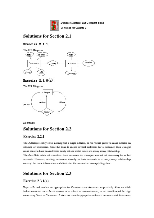
Database Systems: The Complete BookSolutions for Chapter 2Solutions for Section 2.1Exercise 2.1.1The E/R Diagram.Exercise 2.1.8(a)The E/R DiagramKobvxybzSolutions for Section 2.2Exercise 2.2.1The Addresses entity set is nothing but a single address, so we would prefer to make address an attribute of Customers. Were the bank to record several addresses for a customer, then it might make sense to have an Addresses entity set and make Lives-at a many-many relationship.The Acct-Sets entity set is useless. Each customer has a unique account set containing his or her accounts. However, relating customers directly to their accounts in a many-many relationship conveys the same information and eliminates the account-set concept altogether.Solutions for Section 2.3Exercise 2.3.1(a)Keys ssNo and number are appropriate for Customers and Accounts, respectively. Also, we think it does not make sense for an account to be related to zero customers, so we should round the edge connecting Owns to Customers. It does not seem inappropriate to have a customer with 0 accounts;they might be a borrower, for example, so we put no constraint on the connection from Owns to Accounts. Here is the The E/R Diagram,showing underlined keys andthe numerocity constraint.Exercise 2.3.2(b)If R is many-one from E1 to E2, then two tuples (e1,e2) and (f1,f2) of the relationship set for R must be the same if they agree on the key attributes for E1. To see why, surely e1 and f1 are the same. Because R is many-one from E1 to E2, e2 and f2 must also be the same. Thus, the pairs are the same.Solutions for Section 2.4Exercise 2.4.1Here is the The E/R Diagram.We have omitted attributes other than our choice for the key attributes of Students and Courses. Also omitted are names for the relationships. Attribute grade is not part of the key for Enrollments. The key for Enrollements is studID from Students and dept and number from Courses.Exercise 2.4.4bHere is the The E/R Diagram Again, we have omitted relationship names and attributes other than our choice for the key attributes. The key for Leagues is its own name; this entity set is not weak. The key for Teams is its own name plus the name of the league of which the team is a part, e.g., (Rangers, MLB) or (Rangers, NHL). The key for Players consists of the player's number and the key for the team on which he or she plays. Since the latter key is itself a pair consisting of team and league names, the key for players is the triple (number, teamName, leagueName). e.g., JeffGarcia is (5, 49ers, NFL).Database Systems: The Complete BookSolutions for Chapter 3Solutions for Section 3.1Exercise 3.1.2(a)We can order the three tuples in any of 3! = 6 ways. Also, the columns can be ordered in any of 3! = 6 ways. Thus, the number of presentations is 6*6 = 36.Solutions for Section 3.2Exercise 3.2.1Customers(ssNo, name, address, phone)Flights(number, day, aircraft)Bookings(ssNo, number, day, row, seat)Being a weak entity set, Bookings' relation has the keys for Customers and Flights and Bookings' own attributes.Notice that the relations obtained from the toCust and toFlt relationships are unnecessary. They are:toCust(ssNo, ssNo1, number, day)toFlt(ssNo, number, day, number1, day1)That is, for toCust, the key of Customers is paired with the key for Bookings. Since both include ssNo, this attribute is repeated with two different names, ssNo and ssNo1. A similar situation exists for toFlt.Exercise 3.2.3Ships(name, yearLaunched)SisterOf(name, sisterName)Solutions for Section 3.3Exercise 3.3.1Since Courses is weak, its key is number and the name of its department. We do not have arelation for GivenBy. In part (a), there is a relation for Courses and a relation for LabCourses that has only the key and the computer-allocation attribute. It looks like:Depts(name, chair)Courses(number, deptName, room)LabCourses(number, deptName, allocation)For part (b), LabCourses gets all the attributes of Courses, as:Depts(name, chair)Courses(number, deptName, room)LabCourses(number, deptName, room, allocation)And for (c), Courses and LabCourses are combined, as:Depts(name, chair)Courses(number, deptName, room, allocation)Exercise 3.3.4(a)There is one relation for each entity set, so the number of relations is e. The relation for the root entity set has a attributes, while the other relations, which must include the key attributes, have a+k attributes.Solutions for Section 3.4Exercise 3.4.2Surely ID is a key by itself. However, we think that the attributes x, y, and z together form another key. The reason is that at no time can two molecules occupy the same point.Exercise 3.4.4The key attributes are indicated by capitalization in the schema below:Customers(SSNO, name, address, phone)Flights(NUMBER, DAY, aircraft)Bookings(SSNO, NUMBER, DAY, row, seat)Exercise 3.4.6(a)The superkeys are any subset that contains A1. Thus, there are 2^{n-1} such subsets, since each of the n-1 attributes A2 through An may independently be chosen in or out.Solutions for Section 3.5Exercise 3.5.1(a)We could try inference rules to deduce new dependencies until we are satisfied we have them all.A more systematic way is to consider the closures of all 15 nonempty sets of attributes.For the single attributes we have A+ = A, B+ = B, C+ = ACD, and D+ = AD. Thus, the only new dependency we get with a single attribute on the left is C->A.Now consider pairs of attributes:AB+ = ABCD, so we get new dependency AB->D. AC+ = ACD, and AC->D is nontrivial. AD+ = AD, so nothing new. BC+ = ABCD, so we get BC->A, and BC->D. BD+ = ABCD, giving usBD->A and BD->C. CD+ = ACD, giving CD->A.For the triples of attributes, ACD+ = ACD, but the closures of the other sets are each ABCD. Thus, we get new dependencies ABC->D, ABD->C, and BCD->A.Since ABCD+ = ABCD, we get no new dependencies.The collection of 11 new dependencies mentioned above is: C->A, AB->D, AC->D, BC->A, BC->D, BD->A, BD->C, CD->A, ABC->D, ABD->C, and BCD->A.Exercise 3.5.1(b)From the analysis of closures above, we find that AB, BC, and BD are keys. All other sets either do not have ABCD as the closure or contain one of these three sets.Exercise 3.5.1(c)The superkeys are all those that contain one of those three keys. That is, a superkey that is not a key must contain B and more than one of A, C, and D. Thus, the (proper) superkeys are ABC, ABD, BCD, and ABCD.Exercise 3.5.3(a)We must compute the closure of A1A2...AnC. Since A1A2...An->B is a dependency, surely B is in this set, proving A1A2...AnC->B.Exercise 3.5.4(a)Consider the relationThis relation satisfies A->B but does not satisfy B->A.Exercise 3.5.8(a)If all sets of attributes are closed, then there cannot be any nontrivial functional dependenc ies. For suppose A1A2...An->B is a nontrivial dependency. Then A1A2...An+ contains B and thus A1A2...An is not closed.Exercise 3.5.10(a)We need to compute the closures of all subsets of {ABC}, although there is no need to think about the empty set or the set of all three attributes. Here are the calculations for the remaining six sets: A+ = AB+ = BC+ = ACEAB+ = ABCDEAC+ = ACEBC+ = ABCDEWe ignore D and E, so a basis for the resulting functional dependencies for ABC are: C->A and AB->C. Note that BC->A is true, but follows logically from C->A, and therefore may be omitted from our list.Solutions for Section 3.6Exercise 3.6.1(a)In the solution to Exercise 3.5.1 we found that there are 14 nontrivial dependencies, including the three given ones and 11 derived dependencies. These are: C->A, C->D, D->A, AB->D, AB-> C, AC->D, BC->A, BC->D, BD->A, BD->C, CD->A, ABC->D, ABD->C, and BCD->A.We also learned that the three keys were AB, BC, and BD. Thus, any dependency above that does not have one of these pairs on the left is a BCNF violation. These are: C->A, C->D, D->A, AC->D, and CD->A.One choice is to decompose using C->D. That gives us ABC and CD as decomposed relations. CD is surely in BCNF, since any two-attribute relation is. ABC is not in BCNF, since AB and BC are its only keys, but C->A is a dependency that holds in ABCD and therefore holds in ABC. We must further decompose ABC into AC and BC. Thus, the three relations of the decomposition are AC, BC, and CD.Since all attributes are in at least one key of ABCD, that relation is already in 3NF, and no decomposition is necessary.Exercise 3.6.1(b)(Revised 1/19/02) The only key is AB. Thus, B->C and B->D are both BCNF violations. The derived FD's BD->C and BC->D are also BCNF violations. However, any other nontrivial, derived FD will have A and B on the left, and therefore will contain a key.One possible BCNF decomposition is AB and BCD. It is obtained starting with any of the four violations mentioned above. AB is the only key for AB, and B is the only key for BCD.Since there is only one key for ABCD, the 3NF violations are the same, and so is the decomposition.Solutions for Section 3.7Exercise 3.7.1Since A->->B, and all the tuples have the same value for attribute A, we can pair the B-value from any tuple with the value of the remaining attribute C from any other tuple. Thus, we know that R must have at least the nine tuples of the form (a,b,c), where b is any of b1, b2, or b3, and c is any of c1, c2, or c3. That is, we can derive, using the definition of a multivalued dependency, that each of the tuples (a,b1,c2), (a,b1,c3), (a,b2,c1), (a,b2,c3), (a,b3,c1), and (a,b3,c2) are also in R.Exercise 3.7.2(a)First, people have unique Social Security numbers and unique birthdates. Thus, we expect the functional dependencies ssNo->name and ssNo->birthdate hold. The same applies to children, so we expect childSSNo->childname and childSSNo->childBirthdate. Finally, an automobile has a unique brand, so we expect autoSerialNo->autoMake.There are two multivalued dependencies that do not follow from these functional dependencies. First, the information about one child of a person is independent of other information about that person. That is, if a person with social security number s has a tuple with cn,cs,cb, then if there isany other tuple t for the same person, there will also be another tuple that agrees with t except that it has cn,cs,cb in its components for the child name, Social Security number, and birthdate. That is the multivalued dependencyssNo->->childSSNo childName childBirthdateSimilarly, an automobile serial number and make are independent of any of the other attributes, so we expect the multivalued dependencyssNo->->autoSerialNo autoMakeThe dependencies are summarized below:ssNo -> name birthdatechildSSNo -> childName childBirthdateautoSerialNo -> autoMakessNo ->-> childSSNo childName childBirthdatessNo ->-> autoSerialNo autoMakeExercise 3.7.2(b)We suggest the relation schemas{ssNo, name, birthdate}{ssNo, childSSNo}{childSSNo, childName childBirthdate}{ssNo, autoSerialNo}{autoSerialNo, autoMake}An initial decomposition based on the two multivalued dependencies would give us {ssNo, name, birthDate}{ssNo, childSSNo, childName, childBirthdate}{ssNo, autoSerialNo, autoMake}Functional dependencies force us to decompose the second and third of these.Exercise 3.7.3(a)Since there are no functional dependencies, the only key is all four attributes, ABCD. Thus, each of the nontrvial multivalued dependencies A->->B and A->->C violate 4NF. We must separate out the attributes of these dependencies, first decomposing into AB and ACD, and then decomposing the latter into AC and AD because A->->C is still a 4NF violation for ACD. The final set of relations are AB, AC, and AD.Exercise 3.7.7(a)Let W be the set of attributes not in X, Y, or Z. Consider two tuples xyzw and xy'z'w' in the relation R in question. Because X ->-> Y, we can swap the y's, so xy'zw and xyz'w' are in R. Because X ->-> Z, we can take the pair of tuples xyzw and xyz'w' and swap Z's to get xyz'w and xyzw'. Similarly, we can take the pair xy'z'w' and xy'zw and swap Z's to get xy'zw' and xy'z'w.In conclusion, we started with tuples xyzw and xy'z'w' and showed that xyzw' and xy'z'w must also be in the relation. That is exactly the statement of the MVD X ->-> Y-union-Z. Note that the above statements all make sense even if there are attributes in common among X, Y, and Z.Exercise 3.7.8(a)Consider a relation R with schema ABCD and the instance with four tuples abcd, abcd', ab'c'd, and ab'c'd'. This instance satisfies the MVD A->-> BC. However, it does not satisfy A->-> B. For example, if it did satisfy A->-> B, then because the instance contains the tuples abcd and ab'c'd, we would expect it to contain abc'd and ab'cd, neither of which is in the instance.Database Systems: The Complete BookSolutions for Chapter 4Solutions for Section 4.2Exercise 4.2.1class Customer {attribute string name;attribute string addr;attribute string phone;attribute integer ssNo;relationship Set<Account> ownsAcctsinverse Account::ownedBy;}class Account {attribute integer number;attribute string type;attribute real balance;relationship Set<Customer> ownedByinverse Customer::ownsAccts}Exercise 4.2.4class Person {attribute string name;relationship Person motherOfinverse Person::childrenOfFemalerelationship Person fatherOfinverse Person::childrenOfMalerelationship Set<Person> childreninverse Person::parentsOfrelationship Set<Person> childrenOfFemaleinverse Person::motherOfrelationship Set<Person> childrenOfMaleinverse Person::fatherOfrelationship Set<Person> parentsOfinverse Person::children}Notice that there are six different relationships here. For example, the inverse of the relationship that connects a person to their (unique) mother is a relationship that connects a mother (i.e., a female person) to the set of her children. That relationship, which we call childrenOfFemale, is different from the children relationship, which connects anyone -- male or female -- to their children.Exercise 4.2.7A relationship R is its own inverse if and only if for every pair (a,b) in R, the pair (b,a) is also in R. In the terminology of set theory, the relation R is ``symmetric.''Solutions for Section 4.3Exercise 4.3.1We think that Social Security number should me the key for Customer, and account number should be the key for Account. Here is the ODL solution with key and extent declarations.class Customer(extent Customers key ssNo){attribute string name;attribute string addr;attribute string phone;attribute integer ssNo;relationship Set<Account> ownsAcctsinverse Account::ownedBy;}class Account(extent Accounts key number){attribute integer number;attribute string type;attribute real balance;relationship Set<Customer> ownedByinverse Customer::ownsAccts}Solutions for Section 4.4Exercise 4.4.1(a)Since the relationship between customers and accounts is many-many, we should create a separate relation from that relationship-pair.Customers(ssNo, name, address, phone)Accounts(number, type, balance)CustAcct(ssNo, number)Exercise 4.4.1(d)Ther is only one attribute, but three pairs of relationships from Person to itself. Since motherOf and fatherOf are many-one, we can store their inverses in the relation for Person. That is, for each person, childrenOfMale and childrenOfFemale will indicate that persons's father and mother. The children relationship is many-many, and requires its own relation. This relation actually turns out to be redundant, in the sense that its tuples can be deduced from the relationships stored with Person. The schema:Persons(name, childrenOfFemale, childrenOfMale)Parent-Child(parent, child)Exercise 4.4.4Y ou get a schema like:Studios(name, address, ownedMovie)Since name -> address is the only FD, the key is {name, ownedMovie}, and the FD has a left side that is not a superkey.Exercise 4.4.5(a,b,c)(a) Struct Card { string rank, string suit };(b) class Hand {attribute Set theHand;};For part (c) we have:Hands(handId, rank, suit)Notice that the class Hand has no key, so we need to create one: handID. Each hand has, in the relation Hands, one tuple for each card in the hand.Exercise 4.4.5(e)Struct PlayerHand { string Player, Hand theHand };class Deal {attribute Set theDeal;}Alternatively, PlayerHand can be defined directly within the declaration of attribute theDeal. Exercise 4.4.5(h)Since keys for Hand and Deal are lacking, a mechanical way to design the database schema is to have one relation connecting deals and player-hand pairs, and another to specify the contents of hands. That is:Deals(dealID, player, handID)Hands(handID, rank, suit)However, if we think about it, we can get rid of handID and connect the deal and the player directly to the player's cards, as:Deals(dealID, player, rank, suit)Exercise 4.4.5(i)First, card is really a pair consisting of a suit and a rank, so we need two attributes in a relation schema to represent cards. However, much more important is the fact that the proposed schema does not distinguish which card is in which hand. Thus, we need another attribute that indicates which hand within the deal a card belongs to, something like:Deals(dealID, handID, rank, suit)Exercise 4.4.6(c)Attribute b is really a bag of (f,g) pairs. Thus, associated with each a-value will be zero or more (f,g) pairs, each of which can occur several times. We shall use an attribute count to indicate the number of occurrences, although if relations allow duplicate tuples we could simply allow duplicate (a,f,g) triples in the relation. The proposed schema is:C(a, f, g, count)Solutions for Section 4.5Exercise 4.5.1(b)Studios(name, address, movies{(title, year, inColor, length,stars{(name, address, birthdate)})})Since the information about a star is repeated once for each of their movies, there is redundancy. To eliminate it, we have to use a separate relation for stars and use pointers from studios. That is: Stars(name, address, birthdate)Studios(name, address, movies{(title, year, inColor, length,stars{*Stars})})Since each movie is owned by one studio, the information about a movie appears in only one tuple of Studios, and there is no redundancy.Exercise 4.5.2Customers(name, address, phone, ssNo, accts{*Accounts})Accounts(number, type, balance, owners{*Customers})Solutions for Section 4.6Exercise 4.6.1(a)We need to add new nodes labeled George Lucas and Gary Kurtz. Then, from the node sw (which represents the movie Star Wars), we add arcs to these two new nodes, labeled direc tedBy and producedBy, respectively.Exercise 4.6.2Create nodes for each account and each customer. From each customer node is an arc to a node representing the attributes of the customer, e.g., an arc labeled name to the customer's name. Likewise, there is an arc from each account node to each attribute of that account, e.g., an arc labeled balance to the value of the balance.To represent ownership of accounts by customers, we place an arc labeled owns from each customer node to the node of each account that customer holds (possibly jointly). Also, we placean arc labeled ownedBy from each account node to the customer node for each owner of that account.Exercise 4.6.5In the semistructured model, nodes represent data elements, i.e., entities rather than entity sets. In the E/R model, nodes of all types represent schema elements, and the data is not represented at all. Solutions for Section 4.7Exercise 4.7.1(a)<STARS-MOVIES><STAR starId = "cf" starredIn = "sw, esb, rj"><NAME>Carrie Fisher</NAME><ADDRESS><STREET>123 Maple St.</STREET><CITY>Hollywood</CITY></ADDRESS><ADDRESS><STREET>5 Locust Ln.</STREET><CITY>Malibu</CITY></ADDRESS></STAR><STAR starId = "mh" starredIn = "sw, esb, rj"><NAME>Mark Hamill</NAME><ADDRESS><STREET>456 Oak Rd.<STREET><CITY>Brentwood</CITY></ADDRESS></STAR><STAR starId = "hf" starredIn = "sw, esb, rj, wit"><NAME>Harrison Ford</NAME><ADDRESS><STREET>whatever</STREET><CITY>whatever</CITY></ADDRESS></STAR><MOVIE movieId = "sw" starsOf = "cf, mh"><TITLE>Star Wars</TITLE><YEAR>1977</YEAR></MOVIE><MOVIE movieId = "esb" starsOf = "cf, mh"><TITLE>Empire Strikes Back</TITLE><YEAR>1980</YEAR></MOVIE><MOVIE movieId = "rj" starsOf = "cf, mh"><TITLE>Return of the Jedi</TITLE><YEAR>1983</YEAR></MOVIE><MOVIE movieID = "wit" starsOf = "hf"><TITLE>Witness</TITLE><YEAR>1985</YEAR></MOVIE></STARS-MOVIES>Exercise 4.7.2<!DOCTYPE Bank [<!ELEMENT BANK (CUSTOMER* ACCOUNT*)><!ELEMENT CUSTOMER (NAME, ADDRESS, PHONE, SSNO)> <!A TTLIST CUSTOMERcustId IDowns IDREFS><!ELEMENT NAME (#PCDA TA)><!ELEMENT ADDRESS (#PCDA TA)><!ELEMENT PHONE (#PCDA TA)><!ELEMENT SSNO (#PCDA TA)><!ELEMENT ACCOUNT (NUMBER, TYPE, BALANCE)><!A TTLIST ACCOUNTacctId IDownedBy IDREFS><!ELEMENT NUMBER (#PCDA TA)><!ELEMENT TYPE (#PCDA TA)><!ELEMENT BALANCE (#PCDA TA)>]>Database Systems: The CompleteBookSolutions for Chapter 5Solutions for Section 5.2Exercise 5.2.1(a)PI_model( SIGMA_{speed >= 1000} ) (PC)Exercise 5.2.1(f)The trick is to theta-join PC with itself on the condition that the hard disk sizes are equal. That gives us tuples that have two PC model numbers with the same value of hd. However, these two PC's could in fact be the same, so we must also require in the theta-join that the model numbers be unequal. Finally, we want the hard disk sizes, so we project onto hd.The expression is easiest to see if we write it using some temporary values. We start by renaming PC twice so we can talk about two occurrences of the same attributes.R1 = RHO_{PC1} (PC)R2 = RHO_{PC2} (PC)R3 = R1 JOIN_{PC1.hd = PC2.hd AND PC1.model <> PC2.model} R2R4 = PI_{PC1.hd} (R3)Exercise 5.2.1(h)First, we find R1, the model-speed pairs from both PC and Laptop. Then, we find from R1 those computers that are ``fast,'' at least 133Mh. At the same time, we join R1 with Product to connect model numbers to their manufacturers and we project out the speed to get R2. Then we join R2 with itself (after renaming) to find pairs of different models by the same maker. Finally, we get our answer, R5, by projecting onto one of the maker attributes. A sequence of steps giving the desired expression is: R1 = PI_{model,speed} (PC) UNION PI_{model,speed} (Laptop)R2 = PI_{maker,model} (SIGMA_{speed>=700} (R1) JOIN Product)R3 = RHO_{T(maker2, model2)} (R2)R4 = R2 JOIN_{maker = maker2 AND model <> model2} (R3)R5 = PI_{maker} (R4)Exercise 5.2.2Here are figures for the expression trees of Exercise 5.2.1 Part (a)Part (f)Part (h). Note that the third figure is not really a tree, since it uses a common subexpression. We could duplicate the nodes to make it a tree, but using common subexpressions is a valuable form of query optimization. One of the benefits one gets from constructing ``trees'' for queries is the ability to combine nodes that represent common subexpressions.Exercise 5.2.7The relation that results from the natural join has only one attribute from each pair of equated attributes. The theta-join has attributes for both, and their columns are identical.Exercise 5.2.9(a)If all the tuples of R and S are different, then the union has n+m tuples, and this number is the maximum possible.The minimum number of tuples that can appear in the result occurs if every tuple of one relation also appears in the other. Surely the union has at least as many tuples as the larger of R and that is, max(n,m) tuples. However, it is possible for every tuple of the smaller to appear in the other, so it is possible that there are as few as max(n,m) tuples in the union.Exercise 5.2.10In the following we use the name of a relation both as its instance (set of tuples) and as its schema (set of attributes). The context determines uniquely which is meant.PI_R(R JOIN S) Note, however, that this expression works only for sets; it does not preserve the multipicity of tuples in R. The next two expressions work for bags.R JOIN DELTA(PI_{R INTERSECT S}(S)) In this expression, each projection of a tuple from S onto the attributes that are also in R appears exactly once in the second argument of the join, so it preserves multiplicity of tuples in R, except for those thatdo not join with S, which disappear. The DELTA operator removes duplicates, as described in Section 5.4.R - [R - PI_R(R JOIN S)] Here, the strategy is to find the dangling tuples of R and remove them.Solutions for Section 5.3Exercise 5.3.1As a bag, the value is {700, 1500, 866, 866, 1000, 1300, 1400, 700, 1200, 750, 1100, 350, 733}. The order is unimportant, of course. The average is 959.As a set, the value is {700, 1500, 866, 1000, 1300, 1400, 1200, 750, 1100, 350, 733}, and the average is 967. H3>Exercise 5.3.4(a)As sets, an element x is in the left-side expression(R UNION S) UNION Tif and only if it is in at least one of R, S, and T. Likewise, it is in the right-side expressionR UNION (S UNION T)under exactly the same conditions. Thus, the two expressions have exactly the same members, and the sets are equal.As bags, an element x is in the left-side expression as many times as the sum of the number of times it is in R, S, and T. The same holds for the right side. Thus, as bags the expressions also have the same value.Exercise 5.3.4(h)As sets, element x is in the left sideR UNION (S INTERSECT T)if and only if x is either in R or in both S and T. Element x is in the right side(R UNION S) INTERSECT (R UNION T)if and only if it is in both R UNION S and R UNION T. If x is in R, then it is in both unions. If x is in both S and T, then it is in both union. However, if x is neither in R nor in both of S and T, then it cannot be in both unions. For example, suppose x is not in R and not in S. Then x is not in R UNION S. Thus, the statement of when x is in the right side is exactly the same as when it is in the left side: x is either in R or in both of S and T.Now, consider the expression for bags. Element x is in the left side the sum of the number of times it is in R plus the smaller of the number of times x is in S and the number of times x is in T. Likewise, the number of times x is in the right side is the smaller ofThe sum of the number of times x is in R and in S.The sum of the number of times x is in R and in T.A moment's reflection tells us that this minimum is the sum of the number of times x is in R plus the smaller of the number of times x is in S and in T, exactly as for the left side.Exercise 5.3.5(a)For sets, we observe that element x is in the left side(R INTERSECT S) - T。
Chapter 6 - Solid Solutions
Solid Solutions
22. P A I R P R O B A B I L I T Y F U N C T I O N S : THERMODYNAMIC PROPERTIES
A solid phase containing two or more kinds of atom, the relative proportions of which may be varied within limits, is described as a solid solution. Terminal solid solutions are based on the structures of the component metals; intermediate solid solutions may have structures which are different from any of those of the constituents. Most solid solutions are of the substitutional type, in which the different atoms are distributed over one or more sets of common sites, and may interchange positions on the sites. In interstitial solutions, the solute atoms occupy sites in the spaces between the positions of the atoms of the solvent metal; this can only happen when the solute atoms are much smaller than the atoms of the solvent. We must also distinguish between ordered and disordered solid solutions. In the fully ordered state each set of atoms occupies one set of positions, so that the atomic arrangement is similar to that of a compound. This is only possible at compositions where the ratios of the numbers of atoms of different kinds are small integral numbers, but the atomic arrangement may still be predominantly ordered in this way for alloys of arbitrary composition. In disordered solid solutions, the atoms are distributed among the sites they occupy in a nearly random manner. This classification is only approximate, and we shall formulate these concepts more precisely. The definition of the unit cell, and the concept of the translational periodicity of the lattice, lose their strict validity when applied to a disordered solid solution. The mean positions of the atoms, considered as mathematical points, will no longer be specified exactly by (5.8), since there will be local distortions depending on the details of the local configurations. Moreover, a knowledge of the type of atom at one end of a given interatomic vector no longer implies knowledge of the atom at the other end, as it does for a pure component or a fully ordered structure. In a solid solution, precise statements of this nature have to be replaced by statements in terms of the probability of the atom being of a certain type. For many purposes, the strict non-periodicity of the structure is not important, since most physical properties are averages over reasonably large numbers of atoms. Thus the positions of X-ray diffraction maxima depend only on the average unit cell dime Theory of Transformations in Metals and Alloys
HullFund8eCh06ProblemSolutions【范本模板】
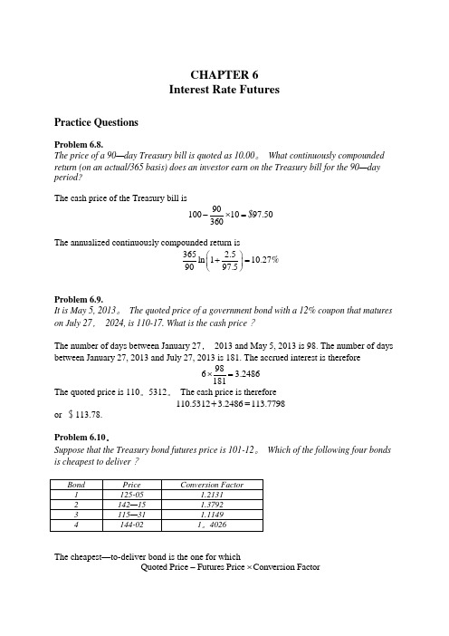
CHAPTER 6Interest Rate FuturesPractice QuestionsProblem 6.8.The price of a 90—day Treasury bill is quoted as 10.00。
What continuously compounded return (on an actual/365 basis) does an investor earn on the Treasury bill for the 90—day period?The cash price of the Treasury bill is 90100109750360$-⨯=.The annualized continuously compounded return is 36525ln 1102790975%.⎛⎫+=. ⎪.⎝⎭Problem 6.9.It is May 5, 2013。
The quoted price of a government bond with a 12% coupon that matures on July 27, 2024, is 110-17. What is the cash price ?The number of days between January 27, 2013 and May 5, 2013 is 98. The number of days between January 27, 2013 and July 27, 2013 is 181. The accrued interest is therefore 98632486181⨯=. The quoted price is 110。
5312。
The cash price is therefore1105312324861137798.+.=.or $113.78.Problem 6.10。
Solutions (6)

Chapter 66.1 When an LED has 2V applied to its terminals, it draws 100mA and produces 2mW of optical power. What is LED ’s conversion efficiency from electrical to optical power? Solution:210020021%200e o e P UI V mA mWP mW P mW η==⨯====6.2 A GaAs laser diode has a 1.5-nm gain linewidth, and its cavity length is 0.5mm, Sketch the output spectrum, including as many details as you can ( for example, the emitted wavelength and the number of the modes ) . Solution:()26230.9100.24222 3.350.5101.560.242c nm nL nm N λλ--⨯∆===⨯⨯⨯=≈6.3 An erbium-doped fiber amplifier has a noise figure of 6 and a gain of 100. The input signal has a 30-dB signal-to-noise ratio and a signal power of 10 W μ. Computer the signal power ( in dBm) and signal-to-noise ratio ( in dB) at the amplifier ’s output.Solution:102010log67.78307.7822.222010lg1000in out in out P W dBmF dB S S F dB dB dBP dBm dBmμ==-===-=-==-+=λ6.4 For an LED, compute the fraction of inject charges that produce photons if 2 mW of optical power are radiated with a drive current of 50mA at 1.3m μ. Solution:198346P 2 1.610 4.2%3106.62610501.310g g i Pe W e W i mW C m s J s mA mηη---⎛⎫=⇒= ⎪⎝⎭⨯⨯==⨯⨯⋅⨯⨯⨯6.5 Source emitting at different wavelength can be multiplexed onto a single fiber, providing multiple channels of information. Assuming a spectral width of 0.02nm for each laser source and a channel separation of 0.05nm (to avoid crosstalk), how many channels can be fitted into the C band.Solution:()():1530~156515651530357000.050.05C band nm nmnm nm N nmnm --===6.6 An erbium- doped fiber amplifiers at 1550nm and is pumped at 980nm. Compute the amplifier efficiency if the only energy loss is due to the fact that it takes one 980nm photon to produce one 1550nm photon. Solution:211298063.2%1550ch nm c nmh λληλλ==== 6.7 Raman scattering results in a downshift in the optical frequency of about 13.2 Thz. If the input wavelength is 1540 nm, compute both the input frequency and the downshifted frequency. Solution:88310193.551550193.5513.2180.35310 1.663180.35shift shift cm s f THz nmf THz THz THz m s m THzλλμ⨯====-=⨯==。
ch06partSolution
Selected Solutions for Exercises inNumerical Methods with Matlab:Implementations and ApplicationsGerald W.RecktenwaldChapter6Finding the Roots of f(x)=0The following pages contain solutions to selected end-of-chapter Exercisesfrom the book Numerical Methods with Matlab:Implementations andApplications,by Gerald W.Recktenwald,c 2000,Prentice-Hall,Upper Saddle River,NJ.The solutions are c 2000Gerald W.Recktenwald.ThePDF version of the solutions may be downloaded or stored or printed onlyfor noncommercial,educational use.Repackaging and sale of these solutionsin any form,without the written consent of the author,is prohibited.The latest version of this PDFfile,along with other supplemental material for the book,can be found at /recktenwald.2Finding the Roots of f(x)=0 6–2The function f(x)=sin(x2)+x2−2x−0.09has four roots in the interval−1≤x≤3.Given the m-file fx.m,which containsfunction f=fx(x)f=sin(x.^2)+x.^2-2*x-0.09;the statement>>brackPlot(’fx’,-1,3)produces only two brackets.Is this result due to a bug in brackPlot or fx?What needs to be changed so that all four roots are found?Demonstrate that your solution works.Partial Solution:The statement>>Xb=brackPlot(’fx’,-1,3)Xb=-0.15790.05262.1579 2.3684returns two brackets.A close inspection of the plot of f(x)reveals that f(x)crosses the x-axis twice near x=1.3.These two roots are missed by brackPlot because there default search interval is too coarse.There is no bug in brackPlot.Implementing a solution using afiner search interval is left as an exercise.6–11Use the bisect function to evaluate the root of the Colebrook equation(see Exercise8) for /D=0.02and Re=105.Do not modify bisect.m.This requires that you write an appropriate function m-file to evaluate the Colebrook equation.Partial Solution:Using bisect requires writing an auxiliary function to evaluate the Cole-brook equation in the form F(f)=0,where f is the friction factor.The following form of F(f)is used in the colebrkz function listed below.F(f)=1√f+2log10/D3.7+2.51Re D√fMany other forms of F(f)will work.function ff=colebrkz(f)%COLEBRKZ Evaluates the Colebrook equation in the form F(f)=0%for use with root-finding routines.%%Input:f=the current guess at the friction factor%%Global Variables:%EPSDIA=ratio of relative roughness to pipe diameter%REYNOLDS=Reynolds number based on pipe diameter%%Output:ff=the"value"of the Colebrook function written y=F(f)%Global variables allow EPSDIA and REYNOLDS to be passed into%colebrkz while bypassing the bisect.m or fzero functionglobal EPSDIA REYNOLDSff=1.0/sqrt(f)+2.0*log10(EPSDIA/3.7+2.51/(REYNOLDS*sqrt(f)));Because the bisect function(unlike fzero)does not allow additional parameters to be passed through to the F(f)function,the values of /D and Re are passed to colebrkz via global variables.Running bisect with colebrkz is left to the reader.For Re=1×10⁵and /D=0.02the solution is f=0.0490.Copyright c 2000,Gerald W.Recktenwald.Photocopying is permitted only for non-commercial educational purposes.Chapter6:Finding the Roots of f(x)=03 6–13Derive the g3(x)functions in Example6.4and Example6.5.(Hint:What is thefixed-pointformula for Newton’s method?)Partial Solution:Thefixed point iteration formulas designated as g3(x)in Example6.4 and Example6.5are obtained by applying Newton’s method.The general form of Newton’smethod for a scalar variable isx k+1=x k−f(x k) f (x k)Example6.4:The f(x)function and its derivative aref(x)=x−x1/3−2f (x)=1−13x−2/3Substituting these expressions into the formula for Newton’s method and simplifying givesx k+1=x k−x k−x1/3k−21−(1/3)x−2/3k=x k(1−(1/3)x−2/3k)−(x k−x1/3k−2)1−(1/3)x−2/3k=x k−(1/3)x1/3k−x k+x1/3k+21−(1/3)x−2/3k=(2/3)x1/3k+21−(1/3)x k=2x1/3k+63−x−2/3kRepeating this analysis for Example6.5is left as an exercise.Copyright c 2000,Gerald W.Recktenwald.Photocopying is permitted only for non-commercial educational purposes.4Finding the Roots of f(x)=0 6–17K.Wark and D.E.Richards(Thermodynamics,6th ed.,1999,McGraw-Hill,Boston,Example 14-2,pp.768–769)compute the equilibrium composition of a mixture of carbon monoxide and oxygen gas at one atmosphere.Determining thefinal composition requires solving3.06=(1−x)(3+x)1/2 x(1+x)1/2for x.Obtain afixed-point iteration formula forfinding the roots of this equation.Implement your formula in a Matlab function and use your function tofind x.If your formula does not converge,develop one that does.Partial Solution:Onefixed point iteration formula is obtained by isolating the factor of (3+x)in the numerator.3.06x(1+x)1/21−x =(3+x)1/2=⇒x=3.06x(1+x)1/21−x2−3=⇒g1(x)=3.06x(1+x)1/21−x2−3Anotherfixed point iteration formula is obtained by solving for the isolated x in the denomi-nator to getx=(1−x)(3+x)1/23.06(1+x)=⇒g2(x)=(1−x)(3+x)1/23.06(1+x)Performing10fixed point iterations with g1(x)givesit xnew1-7.6420163e-012-2.5857113e+003-1.0721050e+014-7.9154865e+015-7.1666488e+026-6.6855377e+037-6.2575617e+048-5.8590795e+059-5.4861826e+0610-5.1370394e+07Thus,g1(x)does not converge.The g2(x)function does converge to the true root of x= 0.340327....Matlab implementations of thefixed point iterations are left as an Exercise. Copyright c 2000,Gerald W.Recktenwald.Photocopying is permitted only for non-commercial educational purposes.Chapter6:Finding the Roots of f(x)=05 6–24Create a modified newton function(say,newtonb)that takes a bracket interval as input instead of a single initial guess.From the bracket limits take one bisection step to determine x0,the initial guess for Newton e the bracket limits to develop relative tolerances on x and f(x)as in the bisect function in Listing6.4.Solution:The newtonb function is listed below.The demoNewtonb function,also listed below, repeats the calculations in Example6.8with the original newton function and with the new newtonb function.Running demoNewtonb gives>>demoNewtonbOriginal newton function:Newton iterations for fx3n.mk f(x)dfdx x(k+1)1-4.422e-018.398e-01 3.526644293139032 4.507e-038.561e-01 3.521380147397333 3.771e-078.560e-01 3.521379706804574 2.665e-158.560e-01 3.5213797068045750.000e+008.560e-01 3.52137970680457newtonb function:Newton iterations for fx3n.mk f(x)dfdx x(k+1)1-4.422e-018.398e-01 3.526644293139032 4.507e-038.561e-01 3.521380147397333 3.771e-078.560e-01 3.521379706804574 2.665e-158.560e-01 3.5213797068045750.000e+008.560e-01 3.52137970680457The two implementations of Newton’s method give identical results because the input to newtonb is the bracket[2,4].This causes the initial bisection step to produce the same initial guess for the Newton iterations that is used in the call to newton.function demoNewtonb%demoNewtonb Use newton and newtonb to find the root of f(x)=x-x^(1/3)-2%%Synopsis:demoNewton%%Input:none%%Output print out of convergence history,and comparison of methodsfprintf(’\nOriginal newton function:\n’);r=newton(’fx3n’,3,5e-16,5e-16,1);fprintf(’\nnewtonb function:\n’);rb=newtonb(’fx3n’,[24],5e-16,5e-16,1);Copyright c 2000,Gerald W.Recktenwald.Photocopying is permitted only for non-commercial educational purposes.6Finding the Roots of f(x)=0 function r=newtonb(fun,x0,xtol,ftol,verbose)%newtonb Newton’s method to find a root of the scalar equation f(x)=0%Initial guess is a bracket interval%%Synopsis:r=newtonb(fun,x0)%r=newtonb(fun,x0,xtol)%r=newtonb(fun,x0,xtol,ftol)%r=newtonb(fun,x0,xtol,ftol,verbose)%%Input:fun=(string)name of mfile that returns f(x)and f’(x).%x0=2-element vector providing an initial bracket for the root%xtol=(optional)absolute tolerance on x.Default:xtol=5*eps%ftol=(optional)absolute tolerance on f(x).Default:ftol=5*eps%verbose=(optional)flag.Default:verbose=0,no printing.%%Output:r=the root of the functionif nargin<3,xtol=5*eps;endif nargin<4,ftol=5*eps;endif nargin<5,verbose=0;endxeps=max(xtol,5*eps);feps=max(ftol,5*eps);%Smallest tols are5*epsif verbosefprintf(’\nNewton iterations for%s.m\n’,fun);fprintf(’k f(x)dfdx x(k+1)\n’);endxref=abs(x0(2)-x0(1));%Use initial bracket in convergence testfa=feval(fun,x0(1));fb=feval(fun,x0(2));fref=max([abs(fa)abs(fb)]);%Use max f in convergence testx=x0(1)+0.5*(x0(2)-x0(1));%One bisection step for initial guessk=0;maxit=15;%Current and max iterationswhile k<=maxitk=k+1;[f,dfdx]=feval(fun,x);%Returns f(x(k-1))and f’(x(k-1))dx=f/dfdx;x=x-dx;if verbose,fprintf(’%3d%12.3e%12.3e%18.14f\n’,k,f,dfdx,x);endif(abs(f/fref)<feps)|(abs(dx/xref)<xeps),r=x;return;endendwarning(sprintf(’root not found within tolerance after%d iterations\n’,k));Copyright c 2000,Gerald W.Recktenwald.Photocopying is permitted only for non-commercial educational purposes.Chapter6:Finding the Roots of f(x)=07 6–27Implement the secant method using Algorithm6.5and Equation(6.13).Test your program by re-creating the results in Example6.10.What happens if10iterations are performed?Replace the formula in Equation(6.13)withx k+1=x k−f(x k)(x k−x k−1)f(x k k−1,whereεis a small number on the order ofεm.How and why does this change the results? Partial Solution:The demoSecant function listed below implements Algorithm(6.5)using Equation(6.13).The f(x)function,Equation6.3,is hard-coded into demoSecant.Note also that demoSecant performs ten iterations without checking for convergence.function demoSecant(a,b);%demoSecant Secant method for finding the root of f(x)=x-x^(1/3)-2=0%Implement Algorithm6.5,using Equation(6.13)%%Synopsis:demoSecant(a,b)%%Input:a,b=initial guesses for the iterations%%Output:print out of iterations;no return values.%copy initial guesses to local variablesxk=b;%x(k)xkm1=a;%x(k-1)fk=fx3(b);%f(x(k))fkm1=fx3(a);%f(x(k-1))fprintf(’\nSecant method:Algorithm6.5,Equation(6.13)\n’);fprintf(’n x(k-1)x(k)f(x(k))\n’);fprintf(’%3d%12.8f%12.8f%12.5e\n’,0,xkm1,xk,fk);for n=1:10x=xk-fk*(xk-xkm1)/(fk-fkm1);%secant formula for updating the rootf=fx3(x);fprintf(’%3d%12.8f%12.8f%12.5e\n’,n,xk,x,f);xkm1=xk;xk=x;%set-up for next iterationfkm1=fk;fk=f;endCopyright c 2000,Gerald W.Recktenwald.Photocopying is permitted only for non-commercial educational purposes.8Finding the Roots of f(x)=0 Running demoSecant with an initial bracket of[3,4](the same bracket used in Example6.10) gives>>demoSecant(3,4)Secant method:Algorithm6.5,Equation(6.13)n x(k-1)x(k)f(x(k))0 3.00000000 4.00000000 4.12599e-011 4.00000000 3.51734262-3.45547e-032 3.51734262 3.52135125-2.43598e-053 3.52135125 3.52137971 1.56730e-094 3.52137971 3.52137971-8.88178e-165 3.52137971 3.52137971-2.22045e-166 3.52137971 3.521379710.00000e+007 3.52137971 3.521379710.00000e+00Warning:Divide by zero.>In/werk/MATLAB_Book/SolutionManual/roots/mfiles/demoSecant.m at line228 3.52137971NaN NaN9NaN NaN NaN10NaN NaN NaNThe secant method has fully converged in6iterations.Continuing the calculations beyond convergence gives afloating point exception because f(x k)−f(x k−1)=0in the denominator of Equation(6.13).In general,it is possible to have f(x k)−f(x k−1)=0before the secant iterations reach convergence.Thus,thefloating point exception exposed by demoSecant should be guarded against in any implementation of the secant method.Implementing thefix suggested in the problem statement is left as an exercise for the reader.Copyright c 2000,Gerald W.Recktenwald.Photocopying is permitted only for non-commercial educational purposes.Chapter6:Finding the Roots of f(x)=09 6–33Write an m-file function to compute h,the depth to which a sphere of radius r,and specific gravity s,floats.(See Example6.12on page281.)The inputs are r and s,and the output ish.Only compute h when s<0.5.The s≥0.5case is dealt with in the following Exercise.If s≥0.5is input,have your function print an error message and stop.(The built-in error function will be useful.)Your function needs to include logic to select the correct root from the list of values returned by the built-in roots function.Partial Solution:The floata function listed below performs the desired computations.We briefly discuss three of the key statements in floata The coefficients of the polynomial are stored in the p vector.Thenc=getreal(roots(p));finds the real roots of the polynomial.The getreal subfunction returns only the real elements of a ing getreal is a defensive programming strategy.The sample calculation in Example6.12obtained only real roots of the polynomial,so getreal would not be necessary in that case.Thek=find(c>0&c<r);statement extracts the indices in the c vector satisfying the criteria0≤c k≤r.Then h=c(k);copies those roots satisfying the criteria to the h vector.No assumption is made that only one root meets the criteria.If more than one root is found a warning message is issued before leaving floata.Testing of floata is left to the reader.Copyright c 2000,Gerald W.Recktenwald.Photocopying is permitted only for non-commercial educational purposes.10Finding the Roots of f(x)=0 function h=floata(r,s)%float Find water depth on a floating,solid sphere with specific gravity<0.5%%Synopsis:h=floata(r,s)%%Input:r=radius of the sphere%s=specific gravity of the sphere(0<s<1)%%Output:h=depth of the sphereif s>=0.5error(’s<0.5required in this version’)elsep=[1-3*r04*s*r^3];%h^3-3*r*h+4*s*r^3=0c=getreal(roots(p));k=find(c>0&c<r);%indices of elements in c such that0<c(k)<rh=c(k);%value of elements in c satisfying above criterionendif length(h)>1,warning(’More than one root found’);end%==============================function cr=getreal(c)%getreal Copy all real elements of input vector to output vector%%Synopsis:cr=getreal(c)%%Input:c=vector of numerical values%%Output cr=vector of only the real elements of c%cr=[]if c has only imaginary elementsn=0;for k=1:length(c)if isreal(c(k))n=n+1;cr(n)=c(k);endendif n==0,cr=[];warning(’No real elements in the input vector’);endCopyright c 2000,Gerald W.Recktenwald.Photocopying is permitted only for non-commercial educational purposes.。
供应链管理英文 Chapter 6 answers to problems
Chapter 6: Designing Global Supply Chain NetworksExercise Solutions1.Answer:Using a decision tree to analyze this decision reveals a dominant answer. Not only does outsourcing to Molectron result in a higher expected incremental profit, but also in every possible outcome, the Molectron option results in a higher profit. Therefore, according to the financial analysis, no matter what the risk tolerance of the management at Moon, they should choose to outsource rather than to increase their own facility.There are other factors that could play into this decision, however, which are harder to quantify. Two are particularly important: the performance of Molectron and the strategic decision regarding where Moon should focus its efforts. It’s possible that Molectron’s quality and delivery performance would be worse than if Moon made the machines themselves. If this is the case, it could counter the financial advantage Molectron presents. Secondly, building the additional plant may increase Moon’s manufacturin g competence and this may be a key to their success down the road. Conversely, the new plant could distract Moon from other aspects of their business making outsourcing more attractive. All these factors should be considered when making the decision. Solution using Decision Tree:Input:Current demand: D0 =10,000Probability of demand goes up in next year: P up = 80%Probability of demand remains the same: P same = 20%Demand increasing rate: u d=150%Increased capacity: M = 10,000Annual fixed cost of new capacity: C fix = $10,000,000Labor cost per server of new capacity: C labor = $500Raw material cost per server: C raw = $ 8,000Labor cost per server by Molectron: C Molectron = $2,000Price per server: P = $15,000Probability of Molectron’s price goes up in the second year: 50%Probability of Molectron’s price remains the same in the second year: 50% Molectron’s cost increasing rate: u c = 120%Output:To draw the decision tree and analyze this problem, we need to calculate for each scenario the total demand and cost per server for both 1st and 2nd years.1st yr. demand if it goes up: D u = D0 * 150% = 15,0001st yr. demand if it remains the same: D d = 10,000There are four scenarios of 2nd demand: D uu, D ud, D dd, D du. The subscripts mean the demand changes. For example, D uu means demand has been going up for two years, and D ud means the demand went up and went down or remained the same.D uu = D0 * u d * u d = 10,000 * 150% * 150% = 22,500D ud = D0 * u d = 10,000 * 150% = 15,000D dd = D0 = 10,000D du = D0 * u d = 10,000 * 150% = 15,000Please note that D uu = 22,500 exceeds the capacity of 20,000, hence Moon Micro can only set 20,000 demand in this scenario. And we should calculate revenue of this scenario accordingly.Independent of demand changes, cost per server by Molectron in the 2nd yr. also has two scenarios. It can remain the same at C Molectron = $2,000, or goes up to C Molectron * u c = $2,000 * 120% = $2,400. Together with the four possible variations due to demand changes, there are eight scenarios in the second year. For each scenario, we need to evaluate its probability, incremental revenue, and profit.We present here how to compute these critical quantifications for one scenario. Analyses for other scenarios are summarized in the table following this analysis. In this scenario, the demand has been going up and up for two years and Molectron raised the cost per server in the second year. This scenario is represented in the decision tree as the upper right-hand node.1. The total probability of D uu and cost per server by Molectron going up is:80% * 80% * 50% = 32%.2. The incremental revenue of this scenario should we take first option is:{ min(capacity, D u ) + min(capacity, D uu) – D0 } * P = $225,000,0003. The incremental revenue of this scenario should we take second option is:( D u + D uu– D0 ) * P = $262,500,000Please note that under the first option, Moon Micro has only 20,000 capacities hence exceeding demand can not be satisfied. However under the second option, Molectron has capacities to handle extra demands.4. The incremental cost of this scenario should we take option one is:C fix * 2 + { min(capacity,D u ) + min(capacity, D uu) – D0 } * (C labor + C raw) =$147,500,0005. The incremental cost of this scenario should we take option two is:( D u - D0 ) * ( C Molectron + C raw) + (D uu– D0) * (C Molectron * u c + C raw ) = $180,000,0006. Hence for the scenario of D uu and cost per server by Molectron also going up, the incremental profit of option one is $225,000,000 - $147,500,000 = $77,500,000; while the incremental profit of option two is $262,500,000 - $180,000,000 = $82,500,000. Similarly we can calculate the profits of option one and option two for each one of the eight scenarios. The details are shown in the following table. The expected incremental profit is calculated by the sum of products of incremental profits and associated probabilities.Table: Incremental Profits for all scenarios scenarios Option 1 Option 21Demand 22500 Revenue $225,000,000 $262,500,000 Molectron cost $2,000 Cost $147,500,000 $175,000,000 Probability 32% Profit $77,500,000 $87,500,0002Demand 22,500 Revenue $225,000,000 $262,500,000 Molectron cost $2,400 Cost $147,500,000 $180,000,000 Probability 32% Profit $77,500,000 $82,500,0003Demand 15,000 Revenue $150,000,000 $150,000,000 Molectron cost $2,000 Cost $105,000,000 $100,000,000 Probability 8% Profit $45,000,000 $50,000,0004Demand 15,000 Revenue $150,000,000 $150,000,000 Molectron cost $2,400 Cost $105,000,000 $102,000,000 Probability 8% Profit $45,000,000 $48,000,0005Demand 15000 Revenue 75,000,000 75,000,000 Molectron cost $2,000 Cost 62,500,000 50,000,000 Probability 8% Profit 12,500,000 25,000,0006Demand 15,000 Revenue 75,000,000 75,000,000 Molectron cost $2,400 Cost 62,500,000 52,000,000 Probability 8% Profit 12,500,000 23,000,0007Demand 10,000 Revenue 0 0 Molectron cost $2,000 Cost 20,000,000 0 Probability 2% Profit -20,000,000 08Demand 10,000 Revenue 0 0 Molectron cost $2,400 Cost 20,000,000 0 Probability 2% Profit -20,000,000 0Solution using Excel Spreadsheet:CELL INPUT SYMBOL FORMULAS QUANTIFIC ATIONC3 Current demand D010,000D18 Probability of demand goes up innext yearP up80%D20 Probability of demand remains thesameP same20%F5 Annual fixed cost of new capacity C fix$10,000,000F6 Labor cost per server of newcapacityC labor$500C5 Raw material cost per server C raw$ 8,000 F9 Labor cost per server by Molectron C Molectron$2,000 C4 Price per server P $15,000 F18 1st yr. demand (up) D u D0 * 150% 15,000 F38 1st yr. demand (down) D d D010,000 I17 2nd yr. demand (up and up) D uu D0 * u d * u d22,500 I21 2nd yr. demand (up and down) D ud D0 * u d 15,000 I41 2nd yr. demand (down and down) D dd D010,000 I33 2nd yr. demand (down and up) D du D0 * u d15,000K17 total probability of D uu and cost perserver by Molectron going upP uu80% * 80% *50%32%N17 incremental revenue of this scenario(first option)R uu_1{ min(capacity, D u )+ min(capacity, D uu)– D0 } * P$225,000,000G17 incremental revenue of this scenario(second option)R uu_2 ( Du + Duu – D0 ) *P$262,500,000N18 incremental cost of this scenario(first option)C uu_1Cfix * 2 +{ min(capacity, Du )+ min(capacity, Duu)– D0 } * (C labor +Craw)$147,500,000O18 incremental cost of this scenario(second option)C uu_2( Du - D0 ) *( CMolectron +Craw) + (Duu – D0)* (CMolectron * uc +Craw )$180,000,000N19 incremental profit of this scenario(first option)F uu_1 R uu_1 – C uu_1$77,500,000O19 incremental profit of this scenario(second option)F uu_2 R uu_2 – C uu_2$82,500,000Workbook Description:Workbook 6-1.xls contains the decision tree showing the:•Basic input data to the analysis•Decision tree with the different potential outcomes•Probabilities of each outcome•Financial impact of each outcome•Expected value calculation for each of the two options that can be chosen.2.Answer:Unlike the Moon Micro example, there is not a dominant choice in the Unipart example. When MRO use is relatively low, the Parts4U option proves to be lower cost. When MRO use is high, AllMRO provides the lower cost. Upon examining the expected value of each, choosing AllMRO has the lower cost.Solution using Decision Tree:Input:Discount rate of Unipart: D = 20%Commission charged by Parts4u: R1 = 5%Commission charged by AllMRO: R2 = 1%Fixed cost charged by AllMRO: C = $10,000,000Current Unipart MRO consumption: M0 = $150,000,000Consumption dropping rate: r = 90%Output:1st yr. consumption (keep): M u = M0 = $150,000,0001st yr. year probability (keep): P u = 75%1st yr. consumption (drop): M d = M0 * r = $135,000,0001st yr. probability (drop): P d = 1 - 75% = 25%2nd yr. consumption (keep and keep): M uu= M0 = 150,000,0002nd yr. probability (keep and keep): P uu = 75% * 50% = 37.5%2nd yr. consumption (keep and drop): M ud= M0 * r = 135,000,0002nd yr. probability (keep and drop): P ud = 75% * 50% = 37.5%2nd yr. consumption (drop and keep): M du= M0 = 150,000,0002nd yr. probability (drop and keep): P du = 25% * 50% = 12.5%2nd yr. consumption (drop and drop): M dd= M0 * r * r = 121,500,0002nd yr. probability (drop and drop): P dd = 25% * 50% = 12.5%As shown above and in the decision tree, there are four demand scenarios. This is independent of which MRO suppliers that Unipart will choose. Hence for each of Parts4u (option 1) and AllMRO(option 2), we need to calculate the NPV cost incurred should Unipart chose it.For the scenario where the demand has been kept at the same level for two successive years, corresponding to the upper-right-hand node in the decision tree and denoted as‘keep and keep’, we calculate the NPV cost as following:Total cost of option Parts4u (keep and keep):C uu_1 = M u * R1 / (1+D) + M uu * R1 /(1+D)^2Total costs of option AllMRO (keep and keep):C uu_2 = C / (1+ D) + M u * R2 / (1+D) + M uu * R2 /(1+D)^2Similarly we can compute NVP costs under other three scenarios for both option one and two. The symbols are also similarly named. These computing results are listed in the following table.Once we know the NVP costs for each scenario, we proceed to calculate the expected cost under each option, and choose the one with lower cost. The calculation is as following:E(Parts4u) = C uu_1 * P uu_1 + C ud_1 * P ud_1 + C du_1 * P du_1 + C dd_1 * P dd_1 = $10,917,969E(AllMRO) = C uu_2 * P uu_2 + C ud_2 * P ud_2 + C du_2 * P du_2 + C dd_2 * P dd_2 = $10,516,927 Since AllMRO provides lower expected cost, it is wise to choose AllMRO.Table: costs for all scenariosdemand scenarios NPV of cost1st yr. 2nd yr. option Parts4u option AllMROkeep keep C uu_1=$11,458,333 C uu_2=$10,625,000keep drop C ud_1=$10,937,500 C ud_2=$10,520,833drop keep C du_1=$10,312,500 C du_2=$10,395,833drop drop C dd_1=$9,843,750 C dd_2=$10,302,083Solution using Excel Spreadsheet:CELL INPUT SYMBOL FORMULAS QUANTIFIC ATIONB3 Discount rate of Unipart D20%E4 Commission charged by Parts4u R15%E8 Commission charged by AllMRO R21%E7 Fixed cost charged by AllMRO C $10,000,000 B31 Current Unipart MRO consumption M0$150,000,000 E21 1st yr. consumption (keep): M u M0$150,000,000 C21 1st yr. probability (keep): P u75%E41 1st yr. consumption (drop) M d M0 * r $135,000,000 C41 1st yr. probability (drop): P d 1 - 75% 25%H16 2nd yr. consumption (keep and keep) M uu M0150,000,000 J16 2nd yr. probability (keep and keep) P uu75% * 50% 37.5%H28 2nd yr. consumption (keep and drop) M ud M0 * r 135,000,000 J28 2nd yr. probability (keep and drop) P ud75% * 50% 37.5%H36 2nd yr. consumption (drop and keep) M du M0 * r 135,000,000 J36 2nd yr. probability (drop and keep) P du25% * 50% 12.5%H48 2nd yr. consumption (drop and drop) M dd M0 * r * r 121,500,000 J48 2nd yr. probability (drop and drop) P dd25% * 50% 12.5%M16 Cost (option one, keep and keep) C uu_1 M u * R1 / (1+D) +M uu * R1 /(1+D)^2$11,458,333N16 Cost (option two, keep and keep): C uu_2 C / (1+ D) + M u *R2 / (1+D) + M uu *R2 /(1+D)^2$10,625,000Workbook Description:Workbook 6-2 .xls contains the decision tree showing the:•Basic input data to the analysis•Decision tree with the different potential outcomes•Probabilities of each outcome•Financial impact of each outcome•Expected value calculation for each of the two options that can be chosen.3.Answer:The high reliability but more costly supplier, Multichem, turns out to have the lower expected cost. This type of outcome is often the case as the increased flexibility that Multichem providesmore than makes up for the significantly higher price that they charge. Although there are situations where Multichem is more expensive (when demand is low in both years), it’s clear that Multichem is the better choice.In addition to the financials, one would also want to consider the quality of the product itself. If Multichem’s product is of higher quality and would lead to less rework on the double cap, this is even more reason to select them as the supplier. Additionally, understanding how quickly each company can respond to changes would be helpful in determining the supplier.Solution using Decision Tree:Input:Discount rate: D = 20 %Cost per unit ( Multichem): C1 = $1.20Cost per unit (Mixemat): C2 = $0.90High demand max (Mixemat) : M = 90,000High demand price (spot market): C3 = $4.00Low demand price (spot market): C4 = $2.00Current sales: S0 = 100,000Probability ( up): P u = 75%Probability ( down): P d = 25%First year sale (up): S u = 110,000First year sale (down): S d = 100,000Output:Second year sale (up and up): S uu = S u* R u = 312,000Probability (up and up): P uu = 75%*75% = 56%Second year sale (up and down): S ud = S d * R d = 99,000Probability (up and down): P ud = 75% * 25% =19%Second year sale (down and up): S du = S d* R u = 120,000Probability (down and up) : P du = 25%*75% = 19%Second year sale (down and down): S dd = S d * R d = 99,000Probability (down and down): P dd = 25% * 25% = 6%As shown above and in the decision tree, there are four demand scenarios. This is independent of which raw material suppliers Alphacap will choose. Hence for each of MultiChem (option 1) and Mixemat (option 2), we need to calculate the NPV cost incurred should Alphacap chose it.For the scenario where the demand will be high in two successive years, corresponding to the upper-right-hand node in the deci sion tree and denoted as ‘up and up’, we calculate the NPV cost as following:Cost (MultiChem, up and up):C uu_1 = S u * C1 / (1 + D) + S uu * C1 / (1 + D) ^2 = $220,000Cost (Mixemat, up and up):C uu_2 = (M* C2 + (S u– M) * C3 )/( 1 + D) + (M* C2 + (S uu– M) * C3)/(1+D)^2 = $307,083The above formula for Mixemat is rather complex, this is because Alphacap needs more than what Mixemat can supply under this scenario. Hence Alphacap has to make up shortfalls from the spot market at a higher price.For other demand scenarios, similar analysis applies, and these are summarized in the following table.Table: Cost for all scenariosdemand scenarios NPV of cost1st yr. 2nd yr. option MultiChem option Mixematup up C uu_1=$220,000 C uu_2=$307,083up down C ud_1=$192,500 C ud_2=$196,042down up C du_1=$200,000 C du_2=$214,583down down C dd_1=$175,000 C dd_2=$131,250And then we proceed to calculate the expected cost under each option, and choose the one with lower cost. The calculation is as following:E(MultiChem) = C uu_1 * P uu_1 + C ud_1 * P ud_1 + C du_1 * P du_1 + C dd_1 * P dd_1 = $208,281 E(Mixemat) = C uu_2 * P uu_2 + C ud_2 * P ud_2 + C du_2 * P du_2 + C dd_2 * P dd_2 = $257,930 Since MultiChem provides lower expected cost, it is wise to choose it.Solution using Excel Spreadsheet: .CELL INPUT SYMBOL FORMULAS QUANTIFIC ATIONC3 Discount rate D 20 %F2 Cost per unit ( Multichem) C1 $1.20F5 Cost per unit (Mixemat) C2 $0.90F6 High demand max (Mixemat) M 90,000 F9 High demand price (spot market) C3 $4.00F10 Low demand price (spot market) C4 $2.00C29 Current sales S0 100,000 D19 Probability ( up) P u 75%D39 Probability ( down) P d 25%F19 First year sale (up) S u 110,000 F39 First year sale (down) S d 100,000 I14 Second year sale (up and up) S uu S u* R u 312,000 K14 Probability (up and up) P uu 75%*75% 56%I26 Second year sale (up and down) S ud S d * R d 99,000 K26 Probability (up and down) P ud 75% * 25% 19%I34 Second year sale (down and up) S du S d* R u 120,000 K34 Probability (down and up) P du 25%*75% 19%I46 Second year sale (down and down) S dd S d * R d 99,000 K46 Probability (down and down) P dd 25% * 25% 6%N14 Cost (option 1, up and up) C uu_1 S u * C1 / (1 + D) +S uu * C1 / (1 + D) ^2$220,000O14 Cost (option 2, up and up) C uu_2 (M* C2 + (S u– M) *C3 )/( 1 + D) + (M*C2 + (S uu – M) *C3)/(1+D)^2$307,083Workbook Description:Workbook 6-3 .xls contains the decision tree showing the:•Basic input data to the analysis•Decision tree with the different potential outcomes•Probabilities of each outcome•Financial impact of each outcome•Expected value calculation for each of the two options that can be chosen.Answer:In making their decision, Bell’s managers must consider the following:•Financial impact of both options in terms of amount that will be paid to either software company to supply either the license or the service, as well as the other costs to implement each alternative•Flexibility provided by each option•Expertise required within the company to execute each option•Expertise built up within the company through the execution of each option•Whether or not the supply chain and its IT system are an area that Bell believes is a core competence of their company•Reliability of each option•Performance and functionality of the solution provided by each option•Changes in personnel that would be required by each option including hiring or firing and their impact on moraleBell should analyze each choice according to the above criteria and, depending on the dynamics of the industry, weight each criterion differently. After taking into account Bell’s tolerance for risk, a quality decision can be made.5.The relevant data for Reliable and the expected outcomes of the decision tree are presented below: Discount factor 0.1Current Capacity in Asia = 2,400,000Current Capacity in N. America = 4,200,000Current Annual Demand in Asia = 2,000,000Current Annual Demand in N.America = 4,000,000Year 1 Demand ProbabilityAsia = 3,000,000 0.7 2,820,000 2,400,000 0.3N. America = 4,400,000 0.5 4,000,000 3,600,000 0.5Year 2 DemandAsia = 4,500,000 0.49 3,976,200 3,600,000 0.212,880,000 0.09N. America = 4,840,000 0.25 4,032,400 3,960,000 0.253,960,000 0.253,240,000 0.26Sale Price of Phone = $ 40.00Variable production cost in Asia = $ 15.00Variable production cost in N. America= $ 17.00Ship between markets $ 3.00Capacity of large addition = 2,000,000Cost of large addition = $18,000,000.00Capacity of small addition = 1,500,000Cost of small addition = $15,000,000.00Given this information, we can calculate the NPV of the expected profits for both the smaller and larger additions. The NPV for the smaller addition is $432,269,587, while the larger addition is $430,529,091.Reliable should only add the 1,500,000 units of capacity to the Asia plant.The problem is worked out in the excel worksheet Problems 6.5,6.6,6.7.xls.6.The relevant data for the European apparel manufacturer and the expected outcomes of the decision tree are presented below:Discount factor 0.1Current Capacity in Italy = 1,000,000Current Capcity in China = 1,000,000Current Annual Demand = 1,900,000Year 1 Currency Exchange ProbabilityChina = 8.05 0.5 7.35 6.65 0.5Year 2 Currency ExchangeChina 9.26 0.25 7.72 7.65 0.257.65 0.25Year 3 Currency ExchangeChina 10.65 0.125 8.10 8.79 0.1258.79 0.1257.27 0.1258.79 0.1257.27 0.1257.27 0.1256.00 0.125Variable production cost in Italy = 10.00Variable production cost in China = 7.00Change in capacity 500,000Cost of moving capacity 2,000,000.00Given this information, we can calculate the NPV of the expected costs of keeping the capacity as is, or moving the capacity to the China plant. The calculation makes the assumption that we maximize production at the cheaper of the two plants, China first and then satisfy the remaining demand from Italy. The NPV for keeping the capacity as is, is $57,529,771, while the NPV of moving capacity to China is $63,256,313.The European manufacturer should keep the capacity as it currently is configured.The problem is worked out in the excel worksheet Problems 6.5,6.6,6.7.xls.7.The relevant data for the chemical manufacturer and the expected outcomes of the decision tree are presented below:Discount factor 0.1N. American CapcityEurope capacity =Current Annual Demand = 4,000,000Year 1 Currency Exchange ProbabilityN. America = 1.20 0.5 1.30 1.40 0.5Year 2 Currency ExchangeN. America 1.38 0.25 1.36 1.14 0.251.61 0.251.33 0.25Year 3 Currency ExchangeN. America 1.58 0.125 1.43 1.31 0.1251.31 0.1251.08 0.1251.85 0.1251.53 0.1251.53 0.1251.26 0.125Variable production cost in Europe = 9.00 eurosVariable production cost in N. America= 10.00 dollarsExchange rate 1.33Cost of building two facilities 2,000,000Given this information, we can calculate the NPV of the expected costs of building all the capacity in N. America or building capacity in both N. America and Europe. The NPV for building all the capacity in N. America, is $216,720,175, while the NPV of building capacity in both N. America and Europe is $158,928,785.The chemical manufacturer should build a plant in both N. America and Europe.The problem is worked out in the excel worksheet Problems 6.5,6.6,6.7.xls.。
- 1、下载文档前请自行甄别文档内容的完整性,平台不提供额外的编辑、内容补充、找答案等附加服务。
- 2、"仅部分预览"的文档,不可在线预览部分如存在完整性等问题,可反馈申请退款(可完整预览的文档不适用该条件!)。
- 3、如文档侵犯您的权益,请联系客服反馈,我们会尽快为您处理(人工客服工作时间:9:00-18:30)。
Chapter 6Variable Costing and Segment Reporting: Tools for ManagementSolutions to Questions6-1Absorption and variable costing differ in how they handle fixed manufacturing overhead. Under absorption costing, fixed manufacturing overhead is treated as a product cost and hence is an asset until products are sold. Under variable costing, fixed manufacturing overhead is treated as a period cost and is expensed on the current period’s income statement.6-2Selling and administrative expenses are treated as period costs under both variable costing and absorption costing.6-3Under absorption costing, fixed manufacturing overhead costs are included in product costs, along with direct materials, direct labor, and variable manufacturing overhead. If some of the units are not sold by the end of the period, then they are carried into the next period as inventory. When the units are finally sold, the fixed manufacturing overhead cost that has been carried over with the units is included as part of that period’s cos t of goods sold.6-4Absorption costing advocates argue that absorption costing does a better job of matching costs with revenues than variable costing. They argue that all manufacturing costs must be assigned to products to properly match the costs of producing units of product with the revenues from the units when they are sold. They believe that no distinction should be made between variable and fixed manufacturing costs for the purposes of matching costs and revenues.6-5Advocates of variable costing argue that fixed manufacturing costs are not really the cost of any particular unit of product. If a unit is made or not, the total fixed manufacturing costs will be exactly the same. Therefore, how can one say that these costs are part of the costs of the products? These costs are incurred to have the capacity to make products during a particular period and should be charged against that period as period costs according to the matching principle.6-6If production and sales are equal, net operating income should be the same under absorption and variable costing. When production equals sales, inventories do not increase or decrease and therefore under absorption costing fixed manufacturing overhead cost cannot be deferred in inventory or released from inventory.6-7If production exceeds sales, absorption costing will usually show higher net operating income than variable costing. When production exceeds sales, inventories increase and under absorption costing part of the fixed manufacturing overhead cost of the current period is deferred in inventory to the next period. In contrast, all of the fixed manufacturing overhead cost of the current period is immediately expensed under variable costing.6-8If fixed manufacturing overhead cost is released from inventory, then inventory levels must have decreased and therefore production must have been less than sales.6-9Under absorption costing net operating income can be increased by simply increasing the level of production without any increase in sales. If production exceeds sales, units of product are added to inventory. These units carry a portion of the current period’s fixed manufacturing overhead costs into the inventory account, reducing the current period’s reported expenses and causing net operating income to increase.6-10Differences in reported net operating income between absorption and variable costing arise because of changing levels of inventory. In lean production, goods are produced strictly to customers’ orders. With production geared to sales, inventories are largely (or entirely) eliminated. If inventories are completely eliminated, they cannot change from one period to another and absorption costing and variable costing will report the same net operating income.6-11 A segment is any part or activity of an organization about which a manager seeks cost, revenue, or profit data. Examples of segments include departments, operations, sales territories, divisions, and product lines.6-12Under the contribution approach, costs are assigned to a segment if and only if the costs are traceable to the segment (i.e., couldbe avoided if the segment were eliminated). Common costs are not allocated to segments under the contribution approach.6-13 A traceable cost of a segment is a cost that arises specifically because of the existence of that segment. If the segment were eliminated, the cost would disappear. A common cost, by contrast, is a cost that supports more than one segment, but is not traceable in whole or in part to any one of the segments. If the departments of a company are treated as segments, then examples of the traceable costs of a department would include the salary of the department’s supervisor, depreciation of machines used exclusively by the department, and the costs of supplies used by the department. Examples of common costs would include the salary of the general counsel of the entire company, the lease cost of the headquarters building, corporate image advertising, and periodic depreciation of machines shared by several departments.6-14The contribution margin is the difference between sales revenue and variable expenses. The segment margin is the amount remaining after deducting traceable fixed expenses from the contribution margin. The contribution margin is useful as a planning tool for many decisions, particularly those in which fixed costs don’t change. The segment margin is useful in assessing the overall profitability of a segment.6-15If common costs were allocated to segments, then the costs of segments would be overstated and their margins would be understated. As a consequence, some segments may appear to be unprofitable and managers may be tempted to eliminate them. If a segment were eliminated because of the existence of arbitrarily allocated common costs, the overall profit of the company would decline and the common cost that had been allocated to the segment would be reallocated to the remaining segments—making them appear less profitable.6-16There are often limits to how far down an organization a cost can be traced. Therefore, costs that are traceable to a segment may become common as that segment is divided into smaller segment units. For example, the costs of national TV and print advertising might be traceable to a specific product line, but be a common cost of the geographic sales territories in which that product line is sold.The Foundational 151. and2.The unit product costs under variable costing and absorption costing are computed as follows:Variable Costing Absorption CostingDirect materials ................................... $24 $24Direct labor ......................................... 14 14Variable manufacturing overhead ......... 2 2Fixed manufacturing overhead($800,000 ÷ 40,000 units) ................ — 20Unit product cost ................................. $40 $603. and4.The total contribution margin and net operating income under variable costing are computed as follows:Sales ................................................. $2,800,000Variable expenses:Variable cost of goods sold(35,000 units × $40 per unit)......... $1,400,000Variable selling and administrative(35,000 units × $4 per unit) .......... 140,000 1,540,000 Contribution margin ............................ 1,260,000Fixed expenses:Fixed manufacturing overhead .......... 800,000Fixed selling and administrative ........ 496,000 1,296,000Net operating loss .............................. $ (36,000)5. and6.The total gross margin and net operating income under absorptioncosting are computed as follows:Sales (35,000 units × $80 per unit) ........................... $2,800,000Cost of goods sold (35,000 units × $60 per unit) ........ 2,100,000Gross margin ........................................................... 700,000Selling and administrative expenses[(35,000 units × $4 per unit) + $496,000] .............. 636,000Net operating income ............................................... $ 64,0007. The difference between the absorption and variable costing netoperating incomes is explained as follows:Variable costing net operating income ...................... $(36,000)Add fixed manufacturing overhead cost deferred ininventory under absorption costing* ..................... 100,000Absorption costing net operating income ................. $ 64,000* The fixed manufacturing overhead deferred in inventory is computed as follows: 5,000 units × $20 per unit = $100,000.8. The break-even point in units is computed as follows:Profit = Unit CM × Q − Fixed expenses$0 = ($80 − $44) × Q − $1,296,000$0 = ($36) × Q − $1,296,000$36Q = $1,296,000Q = $1,296,000 ÷ $36Q = 36,000 unitsThe break-even point is above the actual sales volume; however, inquestion 6, the absorption costing net operating income is $64,000. This counter-intuitive result emerges because $100,000 of fixedmanufacturing overhead is deferred in inventory under absorptioncosting.9. The breakeven point of 36,000 units would remain the same. Thisoccurs because the contribution margin per unit is the same regardless of whether a unit is sold in the East or West region. The total fixed cost also remains unchanged so the break-even point stays at 36,000 units.10. and 11.The variable costing net operating income would be the same as the answer to question 4 as shown below:Sales ................................................. $2,800,000Variable expenses:Variable cost of goods sold(35,000 units × $40 per unit)......... $1,400,000Variable selling and administrative(35,000 units × $4 per unit) .......... 140,000 1,540,000 Contribution margin ............................ 1,260,000Fixed expenses:Fixed manufacturing overhead .......... 800,000Fixed selling and administrative ........ 496,000 1,296,000Net operating loss .............................. $ (36,000)When the number of units produced equals the number of units sold, absorption costing net operating income equals the variable costing net operating income. Therefore, the answer to question 11 is that theabsorption costing net operating loss would be $36,000.12. Absorption costing income will be lower than variable costing income.The variable costing income statement will only include the fixedmanufacturing overhead costs incurred during the second year ofoperations, whereas the absorption costing cost of goods sold willinclude all of the fixed manufacturing overhead costs incurred during the second year of operations plus some of the fixed manufacturingoverhead costs that were deferred in inventory at the end of the prior year.13. The segment margins for the East and West regions are computed as follows:Total East WestSales* ......................................... $2,800,000 $2,000,000 $800,000 Variable expenses** ..................... 1,540,000 1,100,000 440,000 Contribution margin ...................... 1,260,000 900,000 360,000 Traceable fixed expenses .............. 400,000 150,000 250,000 Region segment margin ................ 860,000 $ 750,000 $110,000 Common fixed expenses not traceable to regions($800,000 + $96,000) ............... 896,000 Net operating loss ........................ $ (36,000)* ** East: 25,000 units × $80 per unit = $2,000,000; West: 10,000 units × $80 per unit= $800,000. East: 25,000 units × $44 per unit = $1,100,000; West: 10,000 units × $44 per unit= $440,000.14. Diego has apparently determined that the total gross margin in theWest region equals $200,000. As computed in requirement 1, the unit product cost under absorption costing is $60; therefore the gross margin per unit is $20 ($80 – $60). The West region’s total gross margin of $200,000 (10,000 units × $20 per unit) is less than its traceable fixed expenses of $250,000. This mode of analysis creates the illusion that the West region should be discontinued.The correct way to answer this question is to focus on the informationin the contribution format segmented income statements as follows:Forgone segment margin in the West region ............. $(110,000) Additional contribution margin in East region* .......... 45,000 Decrease in profits if the West region is dropped ...... $ (65,000)* $900,000 × 5% = $45,000.15. The profit impact is computed as follows:Additional advertising .............................................. $(30,000) Additional contribution margin in the West region*.... 72,000 Increase in profits ................................................... $ 42,000 * $360,000 × 20% = $72,000.1. Under absorption costing, all manufacturing costs (variable and fixed)are included in product costs. (All currency values are in thousands of rupees, denoted by R.)Direct materials .................................................................. R120 Direct labor (140)Variable manufacturing overhead (50)Fixed manufacturing overhead (R600,000 ÷ 10,000 units) (60)Absorption costing unit product cost .................................... R3702. Under variable costing, only the variable manufacturing costs areincluded in product costs. (All currency values are in thousands ofrupees, denoted by R.)Direct materials .................................. R120Direct labor (140)Variable manufacturing overhead (50)Variable costing unit product cost ........ R310Note that selling and administrative expenses are not treated as product costs under either absorption or variable costing. These expenses are always treated as period costs and are charged against the currentperiod’s revenue.1. 2,000 units in ending inventory × R60 fixed manufacturing overhead perunit = R120,000.2. The variable costing income statement appears below:Sales ................................................. R4,000,000Variable expenses:Variable cost of goods sold(8,000 units × R310 per unit) ........ R2,480,000Variable selling and administrative(8,000 units × R20 per unit) .......... 160,000 2,640,000 Contribution margin ............................ 1,360,000Fixed expenses:Fixed manufacturing overhead .......... 600,000Fixed selling and administrative ........ 400,000 1,000,000Net operating income ......................... R 360,000The difference in net operating income between variable and absorption costing can be explained by the deferral of fixed manufacturingoverhead cost in inventory that has taken place under the absorption costing approach. Note from part (1) that R120,000 of fixedmanufacturing overhead cost has been deferred in inventory to the next period. Thus, net operating income under the absorption costingapproach is R120,000 higher than it is under variable costing.1. Year 1 Year 2 Year 3Beginning inventories .......... 180 150 160Ending inventories ............... 150 160 200Change in inventories .......... (30) 10 40Fixed manufacturingoverhead in beginninginventories (@$450 perunit) ................................. $ 81,000 $ 67,500 $72,000Fixed manufacturingoverhead in endinginventories (@$450 perunit) ................................. 67,500 72,000 90,000Fixed manufacturingoverhead deferred in(released from)inventories (@$450 perunit) ................................. $(13,500) $ 4,500 $ 18,000Variable costing netoperating income .............. $292,400 $269,200 $251,800Add (deduct) fixedmanufacturing overheadcost deferred in (releasedfrom) inventory underabsorption costing ............ (13,500) 4,500 18,000Absorption costing netoperating income .............. $278,900 $273,700 $269,8002. Because absorption costing net operating income was greater thanvariable costing net operating income in Year 4, inventories must have increased during the year and hence, fixed manufacturing overhead was deferred in inventories. The amount of the deferral is just the difference between the two net operating incomes or $27,000 = $267,200 –$240,200.Total CDDVDSales* ................................................ $750,000 $300,000 $450,000 Variable expenses** ........................... 435,000 120,000 315,000 Contribution margin ............................ 315,000 180,000 135,000 Traceable fixed expenses .................... 183,000 138,000 45,000 Product line segment margin ............... 132,000 $ 42,000 $ 90,000Common fixed expenses not traceableto products ...................................... 105,000 Net operating income .......................... $ 27,000* ** CD: 37,500 packs × $8.00 per pack = $300,000; DVD: 18,000 packs × $25.00 per pack= $450,000. CD: 37,500 packs × $3.20 per pack = $120,000; DVD: 18,000 packs × $17.50 per pack= $315,000.Sales were above the company’s break-even sales and yet the company sustained a loss. The apparent contradiction is explained by the fact that the CVP analysis is based on variable costing, whereas the income reported to shareholders is prepared using absorption costing. Because sales were above the breakeven, the variable costing net operating income would have been positive. However, the absorption costing net operating income was negative. Ordinarily, this would only happen if inventories decreased and fixed manufacturing overhead deferred in inventories was released to the income statement on the absorption costing income statement. This added fixed manufacturing overhead cost resulted in a loss on an absorption costing basis even though the company operated above its breakeven point on a variable costing basis.1. The company is using variable costing. The computations are:Variable Costing Absorption CostingDirect materials .............................. $10 $10Direct labor .................................... 5 5Variable manufacturing overhead .... 2 2Fixed manufacturing overhead($90,000 ÷ 30,000 units) ............. — 3Unit product cost ............................ $17 $20Total cost, 5,000 units ....................2. a. No, $85,000 is not the correct figure to use, because variable costingis not generally accepted for external reporting purposes or for taxpurposes.b. The finished goods inventory account should be stated at $100,000,which represents the absorption cost of the 5,000 unsold units. Thus, the account should be increased by $15,000 for external reportingpurposes. This $15,000 consists of the amount of fixedmanufacturing overhead cost that is allocated to the 5,000 unsoldunits under absorption costing (5,000 units × $3 per unit fixedmanufacturing overhead cost = $15,000).1. a. The unit product cost under absorption costing would be:Direct materials ................................................................ $18 Direct labor . (7)Variable manufacturing overhead (2)Total variable manufacturing costs (27)Fixed manufacturing overhead ($200,000 ÷ 20,000 units) .. 10 Absorption costing unit product cost .................................. $37b. The absorption costing income statement:Sales (16,000 units × $50 per unit) ........................... $800,000 Cost of goods sold (16,000 units × $37 per unit) ........ 592,000 Gross margin ............................................................ 208,000 Selling and administrative expenses[(16,000 units × $2 per unit) + $110,000] .............. 142,000 Net operating income ............................................... $ 66,0002. a. The unit product cost under variable costing would be:Direct materials ................................ $18Direct labor (7)Variable manufacturing overhead (2)Variable costing unit product cost ...... $27b. The variable costing income statement:Sales (16,000 units × $50 per unit) .............. $800,000 Less variable expenses:Variable cost of goods sold(16,000 units × $27 per unit) .................. $432,000Variable selling expense(16,000 units × $2 per unit) ................... 32,000 464,000 Contribution margin ..................................... 336,000 Less fixed expenses:Fixed manufacturing overhead ................... 200,000Fixed selling and administrative ................. 110,000 310,000 Net operating income .................................. $ 26,0003. The price increase appears to be a good idea from an absorption costingperspective because it increases net operating income by $4,000, but a variable costing income statement reveals that the price increase would actually decrease net operating income by $6,000. The incomestatements are shown below:The absorption costing income statement:Sales (15,000 units × $51 per unit) ........................... $765,000Cost of goods sold (15,000 units × $37 per unit) ........ 555,000Gross margin ............................................................ 210,000Selling and administrative expenses[(15,000 units × $2 per unit) + $110,000] .............. 140,000Net operating income ............................................... $ 70,000 The variable costing income statement:Sales (15,000 units × $51 per unit) .............. $765,000Less variable expenses:Variable cost of goods sold(15,000 units × $27 per unit) .................. $405,000Variable selling expense(15,000 units × $2 per unit) ................... 30,000 435,000 Contribution margin ..................................... 330,000Less fixed expenses:Fixed manufacturing overhead ................... 200,000Fixed selling and administrative ................. 110,000 310,000Net operating income .................................. $ 20,000© The McGraw-Hill Companies, Inc., 2013. All rights reserved. Solutions Manual, Chapter 616The completed segmented income statement should appear as follows: Divisions Total Company East WestSales ............................................... $600,000 100.0 $400,000 100.0 $200,000 100.0 Variable expenses ............................ 300,000 50.0 250,000 62.5 50,000 25.0 Contribution margin ......................... 300,000 50.0 150,000 37.5 150,000 75.0 Traceable fixed expenses ................. 190,000 31.7 80,000 20.0 110,000 55.0 Territorial segment margin ............... 110,000 18.3 $ 70,000 17.5 $40,000 20.0Common fixed expenses .................. 60,000 10.0 Net operating income ....................... $ 50,0008.31. Under variable costing, only the variable manufacturing costs areincluded in product costs.Direct materials .................................... $ 60Direct labor (30)Variable manufacturing overhead (10)Variable costing unit product cost .......... $100Note that selling and administrative expenses are not treated as product costs; that is, they are not included in the costs that are inventoried.These expenses are always treated as period costs.2. The variable costing income statement appears below:Sales ................................................. $1,800,000Variable expenses:Variable cost of goods sold(9,000 units × $100 per unit) ......... $900,000Variable selling and administrative(9,000 units × $20 per unit) .......... 180,000 1,080,000 Contribution margin ............................ 720,000Fixed expenses:Fixed manufacturing overhead .......... 300,000Fixed selling and administrative ........ 450,000 750,000Net operating loss .............................. $ (30,000)3. The break-even point in units sold can be computed using thecontribution margin per unit as follows:Selling price per unit ..................... $200Variable cost per unit (120)Contribution margin per unit ......... $ 80Break-even unit sales = Fixed expenses ÷ Unit contribution margin= $750,000 ÷ $80 per unit= 9,375 units1. Under absorption costing, all manufacturing costs (variable and fixed)are included in product costs.Direct materials .................................. $ 60Direct labor (30)Variable manufacturing overhead (10)Fixed manufacturing overhead($300,000 ÷ 10,000 units) (30)Unit product cost ................................ $1302. The absorption costing income statement appears below:Sales (9,000 units × $200 per unit) ............................... $1,800,000 Cost of goods sold (9,000 units × $130 per unit) ............ 1,170,000 Gross margin ................................................................ 630,000 Selling and administrative expenses(9,000 units × $20 per unit) + $450,000 ..................... 630,000 Net operating income ................................................... $ 0 Note: The company apparently has exactly zero net operating income even though its sales are below the break-even point computed in Exercise 6-9. This occurs because $30,000 of fixed manufacturing overhead has been deferred in inventory and does not appear on the income statement prepared using absorption costing.1.Total Geographic MarketCompany South Central North Sales ................................ $1,500,000 $400,000 $600,000 $500,000 Variable expenses ............. 588,000 208,000 180,000 200,000 Contribution margin .......... 912,000 192,000 420,000 300,000 Traceable fixed expenses .. 770,000 240,000 330,000 200,000 Geographic marketsegment margin ............. 142,000 $(48,000) $ 90,000 $100,000 Common fixed expensesnot traceable togeographic markets* ...... 175,000Net operating income(loss) ............................. $ (33,000)*$945,000 – $770,000 = $175,000.2. Incremental sales ($600,000 × 15%) ................... $90,000Contribution margin ratio ($420,000 ÷ $600,000) . × 70%Incremental contribution margin .......................... 63,000Less incremental advertising expense ................... 25,000Incremental net operating income ........................ $38,000Yes, the advertising program should be initiated.1 a. Under variable costing, only the variable manufacturing costs arei ncluded in product costs.Year 1 Year 2 Direct materials .................................... $20 $20Direct labor .......................................... 12 12Variable manufacturing overhead .......... 4 4Variable costing unit product cost .......... $36 $36Note that selling and administrative expenses are not treated asproduct costs; that is, they are not included in the costs that areinventoried. These expenses are always treated as period costs.1 b.Year 1 Year 2 Sales ......................................................... $2,000,000 $2,500,000 Variable expenses:Variable cost of goods sold @ $36 per unit 1,440,000 1,800,000 Variable selling and administrative @ $3per unit ................................................ 120,000 150,000 Total variable expenses ............................... 1,560,000 1,950,000 Contribution margin .................................... 440,000 550,000 Fixed expenses:Fixed manufacturing overhead .................. 200,000 200,000 Fixed selling and administrative ................ 80,000 80,000 Total fixed expenses ................................... 280,000 280,000 Net operating income (loss) ........................ $ 160,000 $ 270,0002 a. The unit product costs under absorption costing:Year 1 Year 2Direct materials .................................... $20 $20Direct labor .......................................... 12 12Variable manufacturing overhead .......... 4 4Fixed manufacturing overhead .............. *4 **5Absorption costing unit product cost ...... $40 $41* $200,000 ÷ 50,000 units = $4 per unit.** $200,000 ÷ 40,000 units = $5 per unit.。