Scaling laws and simulation results for the self--organized critical forest--fire model

合集下载

Research of the parameters of SL scaling law

Research of the parameters of SL scaling law ZHANG Ke;LI Wan-ping【期刊名称】《哈尔滨工业大学学报（英文版）》【年(卷),期】2011(018)004【摘要】As a universal principle of turbulence cascade,scaling law is important in the research on statistics of turbulence.In the thesis PIV system is used to measure the streamwise velocity vector(u') and the component of vorti-city (dv'/dx) in order to analyze the parameters of SL scaling law in the boundary layer at Reθ=2694 (Reθ is obtained by the momentum thickness and free flow velocity).The method of wavelet and statistics are used in this paper.Then,the parameters of SL scaling law are fitted with the scaling law of extended self similarity,extended of refined similarity hypothesis and a new form of refined similarity.At different distances from the wall and different scale,the results show that the fitted curves of u' is in accordance with experimental curves.For dv'/dx,the fitted curves which are fitted with extended of refined similarity hypothesis and a new form of refined similarity is in accordance with experimental curves.【总页数】9页(P104-112)【作者】ZHANG Ke;LI Wan-ping【作者单位】School of Urban Construction, Anhui Radio & TV University, Hefei 230001 , China;Academy of Civil Engineering and Mechanics, Huazhong University of Science and Technology, Wuhan 430074, China 【正文语种】中文【中图分类】O357因版权原因，仅展示原文概要，查看原文内容请购买。

Membrane adhesion via competing receptorligand bonds

c EDP Sciences
2
EUROPHYSICS LETTERS
Fig. 1 – (Left) A membrane containing long and short receptor molecules (top) adhering to a membrane with complementary ligands. In our model, the membranes are discretized into small patches (indicated by dashed lines). A membrane patch can contain a single receptor or ligand molecule. The membrane conformations are described by the local separation zi of each pair i of apposing membrane patches. – (Right) Summing over all possible distributions of receptor and ligand molecules in the partition function leads to an eﬀective double-well potential Vef for the membranes. The potential well at short separations z1 < zi < z2 reﬂects the interactions of the short receptor/ligand bonds, the well at larger separations z3 < zi < z4 reﬂects the interactions of the long receptor/ligand b610020v1 [cond-mat.soft] 1 Oct 2006

Entropy scaling laws for diffusion

a r X iv :cond-m a t /0411357v 1 [c o n d -m a t .s t a t -m e c h ] 12 N o v 2004Entropy scaling laws for diﬀusionSorin Bastea ∗Lawrence Livermore National Laboratory,P.O.BOX 808,Livermore,CA 94550PACS numbers:66.10.Cb Recently,Samanta et al.[1]set out to understand the low density failure of the entropy scaling law for the self-diﬀusion coeﬃcient D conjectured by Dzugutov [2]and to provide a simple alternative.After an interesting derivation,that however contains a number of uncontrolled approximations,they arrive at Eq.7of [1],which reduces for a hard sphere ﬂuid to:D 1−s e /k B (1)with D E =D B /χand D B =3(k B T/πm )1σ2ΓE =B exp (s e /k B )(2)which assumes that the natural length and time scales for diﬀusion are given by a suitably deﬁned hard sphere diameter σand the Enskog collision frequency ΓE =4σ2χρ D B χ=exp (γs e /k B )(3)where we introduced a diﬀerent constant γ.The test of this dependence is shown in Fig.1for hard spheres,with γ=0.8.Furthermore,Eq.3holds for Van der Waals ﬂuids as well [8].Samanta et al.also propose a generalized Stokes-Einstein relation.However,such a relation is hardly necessary given that the usual Stokes-Einstein formula with the ’slip’boundary condition holds well for both hard spheres [9]and Van der Waals ﬂuids [8].This work was performed under the auspices of the U.S.Department of Energy by University of California LawrenceLivermore National Laboratory under Contract No.W-7405-Eng-48.∗Electronic address:bastea2@[1]A.Samanta et al.,Phys.Rev.Lett.92,145901(2004).[2]M.Dzugutov,Nature(London)381,137(1996).[3]S.Chapman,T.G.Cowling,The Mathematical Theory of Non-uniform Gases (Cambridge University Press,Cambridge,England,1970).2012340123−s e /k BD /D EFIG.1:Comparison of the hard spheres diﬀusion coeﬃcient (Ref.[5])-circles,with scaling relation of Ref.[1](Eq.1)-dashed line,Dzugutov scaling law [2](Eq.2)-dot-dashed line,and new entropy scaling (Eq.3)-solid line.[4]J.-P.Hansen,I.R.McDonald,Theory of Simple Liquids ,2nd edition,(Academic Press,London,1986).[5]J.J.Erpenbeck,W.W.Wood,Phys.Rev.A 43,4254(1991).[6]Y.Rosenfeld,Phys.Rev.A 15,2545(1977).[7]E.G.D.Cohen,L.Rondoni,Phys.Rev.Lett.84,394(2000).[8]S.Bastea,Phys.Rev.E 68,031204(2003).[9]B.J.Alder et al.,J.Chem.Phys.53,3813(1970).。

Singularity of the density of states in the two-dimensional Hubbard model from finite size

a r X i v :c o n d -m a t /9503139v 1 27 M a r 1995Singularity of the density of states in the two-dimensional Hubbard model from ﬁnitesize scaling of Yang-Lee zerosE.Abraham 1,I.M.Barbour 2,P.H.Cullen 1,E.G.Klepﬁsh 3,E.R.Pike 3and Sarben Sarkar 31Department of Physics,Heriot-Watt University,Edinburgh EH144AS,UK 2Department of Physics,University of Glasgow,Glasgow G128QQ,UK 3Department of Physics,King’s College London,London WC2R 2LS,UK(February 6,2008)A ﬁnite size scaling is applied to the Yang-Lee zeros of the grand canonical partition function for the 2-D Hubbard model in the complex chemical potential plane.The logarithmic scaling of the imaginary part of the zeros with the system size indicates a singular dependence of the carrier density on the chemical potential.Our analysis points to a second-order phase transition with critical exponent 12±1transition controlled by the chemical potential.As in order-disorder transitions,one would expect a symmetry breaking signalled by an order parameter.In this model,the particle-hole symmetry is broken by introducing an “external ﬁeld”which causes the particle density to be-come non-zero.Furthermore,the possibility of the free energy having a singularity at some ﬁnite value of the chemical potential is not excluded:in fact it can be a transition indicated by a divergence of the correlation length.A singularity of the free energy at ﬁnite “exter-nal ﬁeld”was found in ﬁnite-temperature lattice QCD by using theYang-Leeanalysisforthechiral phase tran-sition [14].A possible scenario for such a transition at ﬁnite chemical potential,is one in which the particle den-sity consists of two components derived from the regular and singular parts of the free energy.Since we are dealing with a grand canonical ensemble,the particle number can be calculated for a given chem-ical potential as opposed to constraining the chemical potential by a ﬁxed particle number.Hence the chem-ical potential can be thought of as an external ﬁeld for exploring the behaviour of the free energy.From the mi-croscopic point of view,the critical values of the chemical potential are associated with singularities of the density of states.Transitions related to the singularity of the density of states are known as Lifshitz transitions [15].In metals these transitions only take place at zero tem-perature,while at ﬁnite temperatures the singularities are rounded.However,for a small ratio of temperature to the deviation from the critical values of the chemical potential,the singularity can be traced even at ﬁnite tem-perature.Lifshitz transitions may result from topological changes of the Fermi surface,and may occur inside the Brillouin zone as well as on its boundaries [16].In the case of strongly correlated electron systems the shape of the Fermi surface is indeed aﬀected,which in turn may lead to an extension of the Lifshitz-type singularities into the ﬁnite-temperature regime.In relating the macroscopic quantity of the carrier den-sity to the density of quasiparticle states,we assumed the validity of a single particle excitation picture.Whether strong correlations completely distort this description is beyond the scope of the current study.However,the iden-tiﬁcation of the criticality using the Yang-Lee analysis,remains valid even if collective excitations prevail.The paper is organised as follows.In Section 2we out-line the essentials of the computational technique used to simulate the grand canonical partition function and present its expansion as a polynomial in the fugacity vari-able.In Section 3we present the Yang-Lee zeros of the partition function calculated on 62–102lattices and high-light their qualitative diﬀerences from the 42lattice.In Section 4we analyse the ﬁnite size scaling of the Yang-Lee zeros and compare it to the real-space renormaliza-tion group prediction for a second-order phase transition.Finally,in Section 5we present a summary of our resultsand an outlook for future work.II.SIMULATION ALGORITHM AND FUGACITY EXPANSION OF THE GRAND CANONICALPARTITION FUNCTIONThe model we are studying in this work is a two-dimensional single-band Hubbard HamiltonianˆH=−t <i,j>,σc †i,σc j,σ+U i n i +−12 −µi(n i ++n i −)(1)where the i,j denote the nearest neighbour spatial lat-tice sites,σis the spin degree of freedom and n iσis theelectron number operator c †iσc iσ.The constants t and U correspond to the hopping parameter and the on-site Coulomb repulsion respectively.The chemical potential µis introduced such that µ=0corresponds to half-ﬁlling,i.e.the actual chemical potential is shifted from µto µ−U412.(5)This transformation enables one to integrate out the fermionic degrees of freedom and the resulting partition function is written as an ensemble average of a product of two determinantsZ ={s i,l =±1}˜z = {s i,l =±1}det(M +)det(M −)(6)such thatM ±=I +P ± =I +n τ l =1B ±l(7)where the matrices B ±l are deﬁned asB ±l =e −(±dtV )e −dtK e dtµ(8)with V ij =δij s i,l and K ij =1if i,j are nearestneigh-boursand Kij=0otherwise.The matrices in (7)and (8)are of size (n x n y )×(n x n y ),corresponding to the spatial size of the lattice.The expectation value of a physical observable at chemical potential µ,<O >µ,is given by<O >µ=O ˜z (µ){s i,l =±1}˜z (µ,{s i,l })(9)where the sum over the conﬁgurations of Ising ﬁelds isdenoted by an integral.Since ˜z (µ)is not positive deﬁnite for Re(µ)=0we weight the ensemble of conﬁgurations by the absolute value of ˜z (µ)at some µ=µ0.Thus<O >µ= O ˜z (µ)˜z (µ)|˜z (µ0)|µ0|˜z (µ0)|µ0(10)The partition function Z (µ)is given byZ (µ)∝˜z (µ)N c˜z (µ0)|˜z (µ0)|×e µβ+e −µβ−e µ0β−e −µ0βn (16)When the average sign is near unity,it is safe to as-sume that the lattice conﬁgurations reﬂect accurately thequantum degrees of freedom.Following Blankenbecler et al.[1]the diagonal matrix elements of the equal-time Green’s operator G ±=(I +P ±)−1accurately describe the fermion density on a given conﬁguration.In this regime the adiabatic approximation,which is the basis of the ﬁnite-temperature algorithm,is valid.The situa-tion diﬀers strongly when the average sign becomes small.We are in this case sampling positive and negative ˜z (µ0)conﬁgurations with almost equal probability since the ac-ceptance criterion depends only on the absolute value of ˜z (µ0).In the simulations of the HSﬁelds the situation is dif-ferent from the case of fermions interacting with dynam-ical bosonﬁelds presented in Ref.[1].The auxilary HS ﬁelds do not have a kinetic energy term in the bosonic action which would suppress their rapidﬂuctuations and hence recover the adiabaticity.From the previous sim-ulations on a42lattice[3]we know that avoiding the sign problem,by updating at half-ﬁlling,results in high uncontrolledﬂuctuations of the expansion coeﬃcients for the statistical weight,thus severely limiting the range of validity of the expansion.It is therefore important to obtain the partition function for the widest range ofµ0 and observe the persistence of the hierarchy of the ex-pansion coeﬃcients of Z.An error analysis is required to establish the Gaussian distribution of the simulated observables.We present in the following section results of the bootstrap analysis[17]performed on our data for several values ofµ0.III.TEMPERATURE AND LATTICE-SIZEDEPENDENCE OF THE YANG-LEE ZEROS The simulations were performed in the intermediate on-site repulsion regime U=4t forβ=5,6,7.5on lat-tices42,62,82and forβ=5,6on a102lattice.The ex-pansion coeﬃcients given by eqn.(14)are obtained with relatively small errors and exhibit clear Gaussian distri-bution over the ensemble.This behaviour was recorded for a wide range ofµ0which makes our simulations reli-able in spite of the sign problem.In Fig.1(a-c)we present typical distributions of theﬁrst coeﬃcients correspond-ing to n=1−7in eqn.(14)(normalized with respect to the zeroth power coeﬃcient)forβ=5−7.5for diﬀer-entµ0.The coeﬃcients are obtained using the bootstrap method on over10000conﬁgurations forβ=5increasing to over30000forβ=7.5.In spite of diﬀerent values of the average sign in these simulations,the coeﬃcients of the expansion(16)indicate good correspondence between coeﬃcients obtained with diﬀerent values of the update chemical potentialµ0:the normalized coeﬃcients taken from diﬀerentµ0values and equal power of the expansion variable correspond within the statistical error estimated using the bootstrap analysis.(To compare these coeﬃ-cients we had to shift the expansion by2coshµ0β.)We also performed a bootstrap analysis of the zeros in theµplane which shows clear Gaussian distribution of their real and imaginary parts(see Fig.2).In addition, we observe overlapping results(i.e.same zeros)obtained with diﬀerent values ofµ0.The distribution of Yang-Lee zeros in the complexµ-plane is presented in Fig.3(a-c)for the zeros nearest to the real axis.We observe a gradual decrease of the imaginary part as the lattice size increases.The quantitative analysis of this behaviour is discussed in the next section.The critical domain can be identiﬁed by the behaviour of the density of Yang-Lee zeros’in the positive half-plane of the fugacity.We expect toﬁnd that this density is tem-perature and volume dependent as the system approaches the phase transition.If the temperature is much higher than the critical temperature,the zeros stay far from the positive real axis as it happens in the high-temperature limit of the one-dimensional Ising model(T c=0)in which,forβ=0,the points of singularity of the free energy lie at fugacity value−1.As the temperature de-creases we expect the zeros to migrate to the positive half-plane with their density,in this region,increasing with the system’s volume.Figures4(a-c)show the number N(θ)of zeros in the sector(0,θ)as a function of the angleθ.The zeros shown in theseﬁgures are those presented in Fig.3(a-c)in the chemical potential plane with other zeros lying further from the positive real half-axis added in.We included only the zeros having absolute value less than one which we are able to do because if y i is a zero in the fugacity plane,so is1/y i.The errors are shown where they were estimated using the bootstrap analysis(see Fig.2).Forβ=5,even for the largest simulated lattice102, all the zeros are in the negative half-plane.We notice a gradual movement of the pattern of the zeros towards the smallerθvalues with an increasing density of the zeros nearθ=πIV.FINITE SIZE SCALING AND THESINGULARITY OF THE DENSITY OF STATESAs a starting point for theﬁnite size analysis of theYang-Lee singularities we recall the scaling hypothesis forthe partition function singularities in the critical domain[11].Following this hypothesis,for a change of scale ofthe linear dimension LLL→−1),˜µ=(1−µT cδ(23)Following the real-space renormalization group treatmentof Ref.[11]and assuming that the change of scaleλisa continuous parameter,the exponentαθis related tothe critical exponentνof the correlation length asαθ=1ξ(θλ)=ξ(θ)αθwe obtain ξ∼|θ|−1|θ|ναµ)(26)where θλhas been scaled to ±1and ˜µλexpressed in terms of ˜µand θ.Diﬀerentiating this equation with respect to ˜µyields:<n >sing =(−θ)ν(d −αµ)∂F sing (X,Y )ν(d −αµ)singinto the ar-gument Y =˜µαµ(28)which deﬁnes the critical exponent 1αµin terms of the scaling exponent αµof the Yang-Lee zeros.Fig.5presents the scaling of the imaginary part of the µzeros for diﬀerent values of the temperature.The linear regression slope of the logarithm of the imaginary part of the zeros plotted against the logarithm of the inverse lin-ear dimension of the simulation volume,increases when the temperature decreases from β=5to β=6.The re-sults of β=7.5correspond to αµ=1.3within the errors of the zeros as the simulation volume increases from 62to 82.As it is seen from Fig.3,we can trace zeros with similar real part (Re (µ1)≈0.7which is also consistentwith the critical value of the chemical potential given in Ref.[22])as the lattice size increases,which allows us to examine only the scaling of the imaginary part.Table 1presents the values of αµand 1αµδ0.5±0.0560.5±0.21.3±0.3∂µ,as a function ofthe chemical potential on an 82lattice.The location of the peaks of the susceptibility,rounded by the ﬁnite size eﬀects,is in good agreement with the distribution of the real part of the Yang-Lee zeros in the complex µ-plane (see Fig.3)which is particularly evident in the β=7.5simulations (Fig.4(c)).The contribution of each zero to the susceptibility can be singled out by expressing the free energy as:F =2n x n yi =1(y −y i )(29)where y is the fugacity variable and y i is the correspond-ing zero of the partition function.The dotted lines on these plots correspond to the contribution of the nearby zeros while the full polynomial contribution is given by the solid lines.We see that the developing singularities are indeed governed by the zeros closest to the real axis.The sharpening of the singularity as the temperature de-creases is also in accordance with the dependence of the distribution of the zeros on the temperature.The singularities of the free energy and its derivative with respect to the chemical potential,can be related to the quasiparticle density of states.To do this we assume that single particle excitations accurately represent the spectrum of the system.The relationship between the average particle density and the density of states ρ(ω)is given by<n >=∞dω1dµ=ρsing (µ)∝1δ−1(32)and hence the rate of divergence of the density of states.As in the case of Lifshitz transitions the singularity of the particle number is rounded at ﬁnite temperature.However,for suﬃciently low temperatures,the singular-ity of the density of states remains manifest in the free energy,the average particle density,and particle suscep-tibility [15].The regular part of the density of states does not contribute to the criticality,so we can concentrate on the singular part only.Consider a behaviour of the typedensity of states diverging as the−1ρsing(ω)∝(ω−µc)1δ.(33)with the valueδfor the particle number governed by thedivergence of the density of states(at low temperatures)in spite of theﬁnite-temperature rounding of the singu-larity itself.This rounding of the singularity is indeedreﬂected in the diﬀerence between the values ofαµatβ=5andβ=6.V.DISCUSSION AND OUTLOOKWe note that in ourﬁnite size scaling analysis we donot include logarithmic corrections.In particular,thesecorrections may prove signiﬁcant when taking into ac-count the fact that we are dealing with a two-dimensionalsystem in which the pattern of the phase transition islikely to be of Kosterlitz-Thouless type[23].The loga-rithmic corrections to the scaling laws have been provenessential in a recent work of Kenna and Irving[24].In-clusion of these corrections would allow us to obtain thecritical exponents with higher accuracy.However,suchanalysis would require simulations on even larger lattices.The linearﬁts for the logarithmic scaling and the criti-cal exponents obtained,are to be viewed as approximatevalues reﬂecting the general behaviour of the Yang-Leezeros as the temperature and lattice size are varied.Al-though the bootstrap analysis provided us with accurateestimates of the statistical error on the values of the ex-pansion coeﬃcients and the Yang-Lee zeros,the smallnumber of zeros obtained with suﬃcient accuracy doesnot allow us to claim higher precision for the critical ex-ponents on the basis of more elaborateﬁttings of the scal-ing behaviour.Theﬁnite-size eﬀects may still be signiﬁ-cant,especially as the simulation temperature decreases,thus aﬀecting the scaling of the Yang-Lee zeros with thesystem rger lattice simulations will therefore berequired for an accurate evaluation of the critical expo-nent for the particle density and the density of states.Nevertheless,the onset of a singularity atﬁnite temper-ature,and its persistence as the lattice size increases,areevident.The estimate of the critical exponent for the diver-gence rate of the density of states of the quasiparticleexcitation spectrum is particularly relevant to the highT c superconductivity scenario based on the van Hove sin-gularities[25],[26],[27].It is emphasized in Ref.[25]thatthe logarithmic singularity of a two-dimensional electrongas can,due to electronic correlations,turn into a power-law divergence resulting in an extended saddle point atthe lattice momenta(π,0)and(0,π).In the case of the14.I.M.Barbour,A.J.Bell and E.G.Klepﬁsh,Nucl.Phys.B389,285(1993).15.I.M.Lifshitz,JETP38,1569(1960).16.A.A.Abrikosov,Fundamentals of the Theory ofMetals North-Holland(1988).17.P.Hall,The Bootstrap and Edgeworth expansion,Springer(1992).18.S.R.White et al.,Phys.Rev.B40,506(1989).19.J.E.Hirsch,Phys.Rev.B28,4059(1983).20.M.Suzuki,Prog.Theor.Phys.56,1454(1976).21.A.Moreo, D.Scalapino and E.Dagotto,Phys.Rev.B43,11442(1991).22.N.Furukawa and M.Imada,J.Phys.Soc.Japan61,3331(1992).23.J.Kosterlitz and D.Thouless,J.Phys.C6,1181(1973);J.Kosterlitz,J.Phys.C7,1046(1974).24.R.Kenna and A.C.Irving,unpublished.25.K.Gofron et al.,Phys.Rev.Lett.73,3302(1994).26.D.M.Newns,P.C.Pattnaik and C.C.Tsuei,Phys.Rev.B43,3075(1991);D.M.Newns et al.,Phys.Rev.Lett.24,1264(1992);D.M.Newns et al.,Phys.Rev.Lett.73,1264(1994).27.E.Dagotto,A.Nazarenko and A.Moreo,Phys.Rev.Lett.74,310(1995).28.A.A.Abrikosov,J.C.Campuzano and K.Gofron,Physica(Amsterdam)214C,73(1993).29.D.S.Dessau et al.,Phys.Rev.Lett.71,2781(1993);D.M.King et al.,Phys.Rev.Lett.73,3298(1994);P.Aebi et al.,Phys.Rev.Lett.72,2757(1994).30.E.Dagotto, A.Nazarenko and M.Boninsegni,Phys.Rev.Lett.73,728(1994).31.N.Bulut,D.J.Scalapino and S.R.White,Phys.Rev.Lett.73,748(1994).32.S.R.White,Phys.Rev.B44,4670(1991);M.Veki´c and S.R.White,Phys.Rev.B47,1160 (1993).33.C.E.Creﬃeld,E.G.Klepﬁsh,E.R.Pike and SarbenSarkar,unpublished.Figure CaptionsFigure1Bootstrap distribution of normalized coeﬃcients for ex-pansion(14)at diﬀerent update chemical potentialµ0for an82lattice.The corresponding power of expansion is indicated in the topﬁgure.(a)β=5,(b)β=6,(c)β=7.5.Figure2Bootstrap distributions for the Yang-Lee zeros in the complexµplane closest to the real axis.(a)102lat-tice atβ=5,(b)102lattice atβ=6,(c)82lattice at β=7.5.Figure3Yang-Lee zeros in the complexµplane closest to the real axis.(a)β=5,(b)β=6,(c)β=7.5.The correspond-ing lattice size is shown in the top right-hand corner. Figure4Angular distribution of the Yang-Lee zeros in the com-plex fugacity plane Error bars are drawn where esti-mated.(a)β=5,(b)β=6,(c)β=7.5.Figure5Scaling of the imaginary part ofµ1(Re(µ1)≈=0.7)as a function of lattice size.αm u indicates the theﬁt of the logarithmic scaling.Figure6Electronic susceptibility as a function of chemical poten-tial for an82lattice.The solid line represents the con-tribution of all the2n x n y zeros and the dotted line the contribution of the six zeros nearest to the real-µaxis.(a)β=5,(b)β=6,(c)β=7.5.。

耗散粒子动力学的简单介绍和应用前景.

耗散粒子动力学的简单介绍和应用前景mg0424112 徐源一．耗散粒子动力学的发展耗散粒子动力学（dissipative particle dynamics）是一种新欣的计算机模拟和描述流体的方法，是对分子动力学（MD）和LGA 模拟的继承和发展。

分子动力学描述的精度较高，但是计算的代价较高，到目前为止，只能用来成功地处理一些简单的流体。

另外，分子动力学应用条件比较苛刻，只能处理两维问题。

LGA （lattice-gas automata）是1986 年Frisch, Hasslacher, Pomeau,Wolfram 提出的描述流体行为的模拟方法，随后Rothman 和Keller 发展这个方法，使它能描绘不能互融的流体行为。

但是LGA模拟有一个不足：模拟中，LGA引入一个重要的概念：格子(lattice), 格子的存在导致伽利略不变性的消失，因此，在描述压缩流体和多相流体时，误差较大。

耗散粒子动力学，集合了以上两种方法的优点：排除了虚拟格子的概念，从而避免了LGA方法的精度的麻烦，另一方面，保留了分离时间步骤的概念，简化了模型，加快了计算的过程。

更重要的是，与前面两者相比较，耗散粒子动力学更容易和精确的模拟了三维状态下流体的行为，因此，具有更重要的意义。

在耗散粒子动力学中，基本颗粒是“格子”，它表示流体材料的一个小区域，相当于MD模拟中我们所熟悉的原子和分子。

假设所有小于一个格子半径的自由度被调整出去只保留格子间粗粒状的相互作用。

在格子之间存在三种力，使得每个格子对保持格子数和线性动量都守恒：简谐守恒相互作用（保守力），表示运动的格子之间的粘滞阻力（耗散力）和为保持不扩散对系统的能量输入（随机力）。

所有这些力都是短程力并具有一个固定的截止半径。

通过选择适当这些力的大小，可得到一个相应于gibbs-cano系统的稳定态。

对于格子运动方程积分可以产生一条通过系统相空间轨迹线，由它可以计算得到所有的热力学可观测量（如密度场，序参量，相关函数，拉伸张量等）。

基于自适应遗传算法的电液弯辊模糊控制系统

在板带材轧制的板形控制系统中，通常采用液压弯辊技术来控制对称浪板形.，具有很多非线性因素，包括伺服阀的不对称性、油温变化引起油液粘度和压缩性的变化、阀控缸的动力方程非线性、放大器死区、库仑摩擦力和管道的影响等，很难精确建立其数学模型. 大量研究资料表明，模糊控制具有很强的鲁棒性，适用于对此类非线性系统的控制.模糊控制是基于人的经验和知识，在选取合适的控制参数时，先验知识就显得很重要，但是这种先验知识往往不够全面，尤其是对非线性系统来说，更加难以获得，这就为设计高精度的模糊控制带来了困难.本文采用自适应遗传算法来全面寻优弯辊模糊控制器参，提高了模糊控制器的动态品质和稳态精度，为进一步提高板形质量奠定了基础.
(Mechanical Engineering Depart m Yanshan University, Qinhuangdao 066004 ,China) ent,
Abstract: In order to improve the efficiency of strip shape' s inner loop and the quality of strip shape, a electr -hydraulic bending fuzzy contr l system based on adaptive genetic algorithm is proposed for 300 four-high o o reversing mill with single stand. The electro hydraulic control system is a typical nonlinear system. In this article , a mathematical model is establishing after considering the nonlinear factor , then the scaling factors, integrating factor,membership function parameters and control r les of a fuzzy controller are optimized by adapu tive genetic algorithm. The results of simulation and experimentation proved that the fuzzy controller optimized is prior to conventional PID controller optimized in robustness performance, dynamic performance and stable precision , which is established the foundation of improving the quality of strip shape. Key words : bending ; adaptive genetic algorithm; fuzzy control; strip shape

一种计算有气隙的磁性元件绕组阻抗的简单办法

Simple analytical approach for the calculation of winding resistance in gapped magnetic components Fermín A. Holguín, Rafael Asensi, Roberto Prieto, José A. CobosUniversidad Politécnica de Madrid (UPM)Centro de Electrónica Industrial (CEI)Madrid, SpainEmail: fermin.holguin@upm.esAbstract—The Dowell expression is the most commonly used method for the analytic calculation of the equivalent resistance in windings of magnetic components. Although this method represents a fast and useful tool to calculate the equivalent resistance of windings, it cannot be applied to components that do not fit with classical 1D assumption, which is the case of gapped magnetic components. These structures can be accurately analyzed using finite-element analysis (FEA) with the time cost that this represents.Modifying the Dowell´s equation, and taking advantage of the orthogonality between skin and proximity effects, a simple solution that allows its application in gapped magnetic components is proposed in this work, which results shows a very good accuracy compared with experimental measurements. Index Terms—Winding resistance, magnetic components, air gap.I.I NTRODUCTIONAccurate estimation of losses in windings of magnetic components used in power electronics applications is a very important task. An imprecise calculation of the equivalent resistances of the windings can lead to under or overestimating the losses in the component, resulting in unexpected temperature rise or a costly component oversize. Several methods have been developed to accurately predict the losses in windingsmade with round conductors [1-6]. The most extended one, often called the Dowell method [1], consists on dividing the windings into portions, considering every portion as an equivalent foil conductor with equal total sectional area and then multiplying the dc resistance of each layer by a corresponding factor to obtain the ac resistance of the winding. This method, however, may have considerable errors at high frequencies [8] and many authors have proposed new models based on modifications of this method [3, 4 and 7]. Another choice to accurately predict the resistance in windings of magnetic components is to use finite element analysis (FEA) tools to model and simulate the component [9-11]. These tools are considered to provide reliable results with the disadvantage of relatively large simulation time.When it comes to gapped magnetic components, Dowell based methods cannot be properly applied because they are only valid when the windings of the magnetic component are arranged in a specific way and the magnetic field along the window breath can be considered as one-dimensional (1D), which clearly is not the case of gapped components. In [12] a solution to calculate the power losses in round conductors in gapped magnetic components is proposed but it can require a big computation time as it uses the mirror-image method [13] to obtain the magnetic field over the considered conductor and the winding must be considered turn by turn.When a fast computation of the equivalent resistance of the windings is needed, the simplicity of the Dowell’s method represents a huge advantage because it can be easily integrated in magnetic modeling and design tools without, practically, penalize the computation time. This simplicity, however, cannot be exploited when gapped magnetic components are being analyzed forcing the designer to use a time consuming calculation method in order to predict the winding resistance in this kind of components. In this paper, a correction factor, based on geometrical parameters of the windings and the local magnetic field in the component, which improves the calculation of the equivalent resistance of the windings in gapped magnetic components (using the foundations of Dowell’s method) is proposed. The results of the proposed method have small errors compared with measurements in many cases.II.ESTIMATING PROXIMITY EFFECT LOSSESA.The Dowell’s equationIn the Dowell method, a layer of round conductors with diameter D is replaced by a single foil conductor with thickness d equal to √⁄ (see figure 1). Given that the equivalent foil conductor has been extended to become a conductor with equal height of the window bread b, it must be corrected by a parameter η, called the porosity factor, equal to ()⁄, where s is the spacing between turns, in order to match its dc resistance with the original winding [1, 2]. Then the ac resistance of the m th layer can be calculated with expression (1), where Rac and Rdc are the ac and dc resistance of a given layer in the winding, m is the number of the layer in consideration and X is equal to ⁄, being δthe skin depth defined as √⁄ where µand σare, respectively, thepermeability and conductivity of the conductor and f is the frequency of the sinusoidal current.[()](1)a)b)c)Figure 1. Obtaining the equivalent foil conductor from round conductors: a)layer of round conductors with diameter D, b) spaced square conductors ofwidth d and c) the equivalent foil conductor of width d’ and height b.Expression (1) assumes constant field along the windowbreath and the factor( )⁄, from now on F(m),represents the increment of the field due to the contribution ofthe corresponding layer to the next one respect to the existingfield. As skin and proximity effects are orthogonal [2, 3], it ispossible to calculate both effects separately and (1) can besplit as follows:[](2)[ ()](3)As Dowell’s approach only considers the proximity effectbetween layers, its influence over the equivalent resistance ofa winding with only one equivalent layer would be zero,neglecting the actual proximity effec t between turns “inside”the equivalent layer. As a consequence, the relative errorbetween the calculated resistances, by means of Dowellmethod and FEA tools, goes bigger as the frequency increases.This situation can be seen in figure 2, where the calculatedresistance of a given component is compared with FEAresults.Moreover, if there is a gap in the magnetic core, thewindings, besides the proximity effect between turns, will beinfluenced by the fringing field of the gap which will bereflected as an increment of the equivalent resistance (seefigure 3). In this situation, although the windings could easilybe converted into equivalent layers, the magnetic field alongthe window breath cannot be considered as one-dimensionaland, therefore, Dowell’s method cannot be properly applied.(a)(b)Figure 2. (a) Axis-symmetric representation of a magnetic component with 13turns (D = 0.6 mm and s = 0.1 mm) and (b) calculatedand FEA simulatedequivalent resistance vs. frequency.Figure 3. Calculated and FEA simulated equivalent resistance vs. frequency inthe component 2a with a central gap of 0.4 mm.Frequency (MHz)Resistance(Ohm)Frequency (MHz)Resistance(Ohm)B.Modifying the Dowell’s modelIf we neglect the edge effect of the core over the conductors and consider that the skin effect contribution in the equivalent resistance of the component only depends on the frequency and the characteristics of the conductive material, it can be assumed that gap and proximity effects are the main contributors of errors in the calculated resistance. In this order, we can divide the total proximity effect (including gap effect) in two components: intra-layer proximity and inter-layer proximity which are, respectively, the proximity effect between turns within an equivalent layer and the proximity effect between layers (the gap effect has been included in this component). Since F(m), in expression (3), represents the increment of the H field from one layer to another, we can modify this factor in order to take into account the influence of both components of the proximity effect and correct the calculations and its contribution in the equivalent resistance of the winding.To do that, many 2-D and 3-D FEA simulations have been run in order to establish a relationship between the current H field along the layers and winding area and the influence of geometrical characteristics of the winding in its equivalent resistance. For this, a simple procedure was followed:1-Three groups of magnetic components, divided in coreless, gapped and non-gapped, are modeled andsimulated.2-The results are processed in order to clear the proximity factor from expression (1) and the resultinginformation is used to make a mathematical regressionand fit the data into a new chosen proximity factor,F X(m), which will replace F(m) in (3) of the form:() ( )(4) Where() (5)() (6) With m equal to the corresponding layer.3-Finally, the coefficients of the new factor are expressed in terms of geometrical and magnetic characteristics ofthe winding.C.Defining the coefficientsThe coefficients a1, a0, b2, b1, and b0in (5) and (6) have been expressed, through a data fitting process from FEA results, as functions of geometrical parameters (diameter of the conductors, distance between conductors and layers) and magnetic field H around the equivalent layer and its distance from the air gap.First, the first component of the proximity factor, the intra-layer factor, was evaluated. For this case, since there should not be any core influence over the windings, a group of coreless components (with one layer of conductors) was simulated in 2D and 3D FEA tools and the coefficients were related with the winding structure (diameter of the conductors and distance between turns). Then, in order to evaluate the second component of the proximity factor, the magnetic core was included in the analysis and the group of non-gapped and multilayered components was simulated to expand the correction factor to multilayered windings in such a way that a1and b1 could be expressed as a function of the wire diameter, distance between turns and layers, d t and d l respectively, and the number of the corresponding layer, m, and b2 as a constant according to expressions (7), (8) and (9), respectively. Coefficients a0 and b0, as the gap influence is not yet taken into account, can be considered as constants equal to -1.171 and 0.12 respectively. At this point, as the proximity factor has been corrected with the intra-layer proximity effect, the modified model can be used to calculate equivalent resistance in both coreless and non-gapped magnetic components.( )(7)(8)(9) Coefficients a0and b0could be modified according to the information of the fringing field and the distance from the corresponding layer to the air gap in order to include its influence in the calculations. If we take, as a reference, the magnetic field, H a, produced by an air cored component with one layer of N turns carrying a current I, and having in consideration that the magnetic field intensity due to the air gap over a given conductor is inversely proportional to its distance from the gap, x, a0and b0can be expressed as functions of the magnetic field factor, H, the number of layers, n, the corresponding layer, m, the length of the reference air cored layer, l a and the length of the air gap, l g, as follows:⁄⁄(10)⁄⁄(11)[()][ ( )](12)()(13)()(14)D.Model validitySince the study was focused on the windings structure and the effect of the air gap over the equivalent resistance, and considering that the model has been developed from the basis of Dowell’s method, it is considered that the characteristics ofthe magnetic core (permeability, shape) have no influence over the calculated resistance of the windings. The study, therefore, was carried out based on the results of FEA simulations of many components in which no especial care has been taken in the shape of the core or the magnetic material used for the simulations. Actually, all FEA simulations were run with POT cores, of different sizes, and a linear generic ferrite with a relative permeability equal to 1000. The windings of the simulated components were modeled with copper round conductors with diameters from 0.1 mm to 1 mm, distance between turns from 0.09 mm to 3 mm and distance between layers from 0.1 mm to 2 mm. Outside these conditions, the validity of the described method has not been tested.III.R ESULTSTo state the accuracy of the proposed model, the equivalent resistance of several components has been calculated using the described model and compared with measurements. The tested devices are coreless (air-cored) inductors of 1 and 2 layers and gapped inductors of 1 and 4 layers (with 15 turns per layer) made with AWG24 magnet wire placed in a RM8/I core (material 3F3 from FERROXCUBE) with two different air gaps: 0.4 mm and 2.2mm. The impedances of all components were measured with a precision impedance analyzer (Agilent 4294A) in a frequency range from 40Hz to 2MHz.The R dc of each layer of conductors was calculated according to its number of turns, length and section of the wire with a copper resistivity for 25°C (room temperature). The calculated resistance in coreless and gapped components, using the proposed method, is compared with classical Dowell, 2-D FEA simulations and experimental data in figures 4 and 5 respectively, where a good agreement with measurements can be appreciated (for visibility issues, due to the resonance between the inductance and parasitic capacitance, the equivalent resistance in the full frequency range of the measurement is not showed in figure 5). Although the results are being compared with Dowell, this information is merely informative because, considering the nature of the considered components, the classical method of Dowell cannot be properly applied to these configurations. For similar reasons, the results obtained for these particular components (gapped) cannot be compared with others solutions, but [12] and FEA (here they are compared with FEA only), because they do not include the influence of the fringing field over conductors.The results in figure 5 do not include the effect of the resonance between the inductance and the parasitic capacitance of the windings. If we include the measured inductance and parasitic capacitance of the component in figure 2d (182.95 µH and 27.03 pF respectively) in the results, the calculated equivalent resistance matches very well with measurements for this component (see figure 6).(a)(b)Figure 4. Equivalent resistance vs. frequency in a coreless component with 9 turns, turn diameter of 8.4 mm, 0.1 mm of distance between turns and wire diameter of 0.6 mm. (a) Single layer and (b) two parallel layers.Frequency (MHz)Resistance(Ohm)Frequency (MHz)Resistance(Ohm)(a)(b)(c)(d)Figure 5. Comparison of equivalent resistance vs. frequency predicted by the proposed model with classic Dowell, 2-D FEA simulations and measurements. (a)And (b) windings of 1 and 4 layers respectively with air gap of 0.4 mm, (c) and (d) windings of 1 and 4 layers respectively with air gap of 2.2 mm.I.C ONCLUSIONSA cor rection factor that allows the application of Dowell’s method in the estimation of equivalent resistance in windings of gapped magnetic components is proposed. This approach has been studied based in 2D and 3D FEA simulations which results has been used to develop a fast and simple semi-empirical method that shows good agreement with measurements in the considered cases. As the relevant coefficients of the proposed method are related with magnetic and geometrical characteristics of the component it can be used, besides gapped components, in other configuration such non-gapped and core-less components but, as it has been developed based on Dowell’s approach, it is restricted to “layered” windings structures.Also, as the model was developed from the basis of Dowell’s method, it is considered that the characteristics of the magnetic core have no influence over the calculated resistance (edge effect neglected). However, from 2D FEA results, it has been observed that the permeability of the magnetic core does have influence over the equivalent resistance of the windings and, therefore, it should be included in the model. In gapped components the influence of the air gap in the equivalent resistance of the windings is much higher than edge effect and it can be neglected. In non-gapped components, edge effect can be significant as the relative permeability of the magnetic material and frequency increase and the functions to obtain the coefficients related with magnetic properties might not be accurate.Frequency (MHz)R e s i s t a n c e (O h m )Frequency (MHz)R e s i s t a n c e (O h m )Frequency (MHz)R e s i s t a n c e (O h m )Frequency (MHz)R e s i s t a n c e (O h m )Figure 6. Equivalent resistance vs. frequency predicted by the proposed model including the effect of the resonance in component of 4 layers with air gap of 2.2 mm.R EFERENCES[1] P.L. Dowell, “Ef fects of eddy currents in transformerwindings”, Proceedings of the IEE , vol. 113, no. 8, pp. 1387–1394, Aug. 1966.[2] J. A. Ferreira, “Improved analytical modeling of conductivelosses in magnetic components”, IEEE Transactions on Power Electronics , vol. 9, no. 1, pp. 127–31, Jan. 1994.[3] Xi Nan and Charles R. Sullivan, “An improved calculation ofproximity effect loss in high frequency windings of round conductors”, in 34th Annual IEEE Power Electronics Specialists Conference , 2003, vol. 2, pp. 853–860.[4] Xi Nan and Charles R. Sullivan, “Simplified high -accuracycalculation of eddy-current loss in round-wire windings”, in 35th Annual IEEE Power ElectronicsSpecialists Conference , 2004, vol. 2, pp. 873 – 879.[5] M.P. Perry, “Multiple layer serie s connected winding design forminimum losses”, IEEE Transactions on Power Apparatus and Systems, vol. PAS-98, pp. 116-123, Jan. /Feb. 1979.[6] M.P. Perry, “Multiple layer parallel connected air -core inductordesign”, IEEE Transactions on Power Apparatus and Systems, vol. PAS-98, pp. 1387-1393, Jul./Aug. 1979.[7] F. Robert, P. Mathys and J. P. Schauwers “A closed -formformula for 2-D ohmic losses calculations in SMPS transformer foils”, IEEE Transactions on Power Electronics, vol. 16, pp. 437-444, May 2001.[8] R. Prieto, J. A. Oliver, J. A. Cobos, J. Uceda and M. Christini“Errors obtained when 1D magnetic component models are not properly applied ”, Annual IEEE Applied Power Electronics and Expositions, 1999, vol. 1, pp. 206-212.[9] R. Asensi, J.A. Cobos, O. García, R. Prieto and J. Uceda “Afull procedure to model high frequency transformer windings”, 25th Annual IEEE Power Electronics Specialists Conference , 1994, vol. 2, pp. 856-863.[10] R. Asensi, R. Prieto, J.A. Cobos and J. Uc eda “Modeling high -frequency multiwinding magnetic components using finite-element analysis”, IEEE Transactions on Magnetics , vol. 43, no. 10, pp. 3840-3850, 2007.[11] R. Prieto, R. Asensi, C. Fernandez, J.J.A. Oliver and J.A.Cobos, “Bridging the gap be tween FEA field solution and the magnetic component model”, IEEE Transactions on Power Electronics , vol. 22, no. 3, pp. 943-951, 2007.[12] Chen Wei, Huang Xiaosheng and Zheng Juanjuan “Improvedwinding loss theoretical calculation of magnetic component with air gap”, 7th International Power Electronics and Motion Control Conference , 2012, vol. 1, pp. 471-475.[13] Jiankun Hu and Charles R. Sullivan “Optimization of shapesfor round-wire high-frequency gapped-inductor w indings”, 33th Annual IEEE Industry Applications Conference , 1998, vol. 2, pp. 907-912.Frequency (MHz)R e s i s t a n c e (O h m )。

The scaling laws of human travel

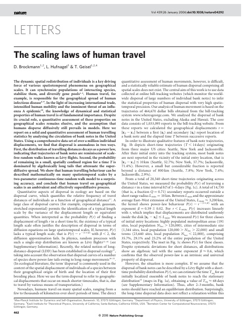
The scaling laws of human travelD.Brockmann 1,2,L.Hufnagel 3&T.Geisel 1,2,4The dynamic spatial redistribution of individuals is a key driving force of various spatiotemporal phenomena on geographical scales.It can synchronize populations of interacting species,stabilize them,and diversify gene pools 1–3.Human travel,for example,is responsible for the geographical spread of human infectious disease 4–9.In the light of increasing international trade,intensiﬁed human mobility and the imminent threat of an inﬂu-enza A epidemic 10,the knowledge of dynamical and statistical properties of human travel is of fundamental importance.Despite its crucial role,a quantitative assessment of these properties on geographical scales remains elusive,and the assumption that humans disperse diffusively still prevails in models.Here we report on a solid and quantitative assessment of human travelling statistics by analysing the circulation of bank notes in the United ing a comprehensive data set of over a million individual displacements,we ﬁnd that dispersal is anomalous in two ways.First,the distribution of travelling distances decays as a power law,indicating that trajectories of bank notes are reminiscent of scale-free random walks known as Le´vy ﬂights.Second,the probability of remaining in a small,spatially conﬁned region for a time T is dominated by algebraically long tails that attenuate the super-diffusive spread.We show that human travelling behaviour can be described mathematically on many spatiotemporal scales by a two-parameter continuous-time random walk model to a surpris-ing accuracy,and conclude that human travel on geographical scales is an ambivalent and effectively superdiffusive process.Quantitative aspects of dispersal in ecology are based on the dispersal curve,which quantiﬁes the relative frequency of travel distances of individuals as a function of geographical distance 11.A large class of dispersal curves (for example,exponential,gaussian,stretched exponential)permits the identiﬁcation of a typical length scale by the variance of the displacement length or equivalent quantities.When interpreted as the probability P (r )of ﬁnding a displacement of length r in a short time d t ,the existence of a typical length scale often justiﬁes the description of dispersal in terms of diffusion equations on large spatiotemporal scales.If,however,P (r )lacks a typical length scale,that is P (r ),r 2(1þb )with b ,2,the diffusion approximation fails.In physics,random processes withsuch a single-step distribution are known as Le´vy ﬂights 12–16(see Supplementary Information).Recently,the related notion of long-distance-dispersal (LDD)has been established in dispersal ecology 17,taking into account the observation that dispersal curves of a number of species show power-law tails owing to long-range movements 18–21.(In ecological literature,the term ‘dispersal’is commonly used in the context of the spatial displacement of individuals of a species between their geographical origin of birth and the location of their ﬁrst breeding place.Here we use the term dispersal to refer to geographi-cal displacements that occur on much shorter timescales,that is,due to travel by various means of transportation.)Nowadays,humans travel on many spatial scales,ranging from a few to thousands of kilometres over short periods of time.The directquantitative assessment of human movements,however,is difﬁcult,and a statistically reliable estimate of human dispersal comprising all spatial scales does not exist.The central aim of this work is to use data collected at online bill-tracking websites (which monitor the world-wide dispersal of large numbers of individual bank notes)to infer the statistical properties of human dispersal with very high spatio-temporal precision.Our analysis of human movement is based on the trajectories of 464,670dollar bills obtained from the bill-tracking system .We analysed the dispersal of bank notes in the United States,excluding Alaska and Hawaii.The core data consists of 1,033,095reports to the bill-tracking website.From these reports we calculated the geographical displacements r ¼j x 22x 1j between a ﬁrst (x 1)and secondary (x 2)report location of a bank note and the elapsed time T between successive reports.In order to illustrate qualitative features of bank note trajectories,Fig.1b depicts short-time trajectories (T ,14days)originating from three major US cities:Seattle,New York and Jacksonville.After their initial entry into the tracking system,most bank notes are next reported in the vicinity of the initial entry location,that is j x 22x 1j #10km (Seattle,52.7%;New York,57.7%;Jacksonville,71.4%).However,a small but considerable fraction is reported beyond a distance of 800km (Seattle,7.8%;New York,7.4%;Jacksonville,2.9%).From a total of 20,540short-time trajectories originating across the United States,we measured the probability P (r )of traversing a distance r in a time interval d T of 1–4days (Fig.1c).A total of 14,730(that is,a fraction Q ¼0.71)secondary reports occurred outside a short range radius L min ¼10km.Between L min and the approximate average East–West extension of the United States,L max <3,200km,the kernel shows power-law behaviour P (r ),r 2(1þb )with an exponent b ¼0.59^0.02.For r ,L min ,P (r )increases linearly with r ,which implies that displacements are distributed uniformly inside the disk j x 22x 1j #L min .We measured P (r )for three classes of initial entry locations:highly populated metropolitan areas (191sites,local population N loc .120,000),cities of intermediate size (1,544sites,local population 120,000.N loc .22,000)and small towns (23,640sites,local population N loc ,22,000),comprising 35.7%,29.1%and 25.2%of the entire population of the United States,respectively.The inset in Fig.1c shows P (r )for these classes.Despite systematic deviations for short distances,all distributions show an algebraic tail with the same exponent b <0.6,which conﬁrms that the observed power-law is an intrinsic and universal property of dispersal.However,the situation is more complex.If we assume that thedispersal of bank notes can be described by a Le´vy ﬂight with a short-time probability distribution P (r ),we can estimate the time T eq for an initially localized ensemble of bank notes to reach the stationary distribution 22(maps in Fig.1a),obtaining a value of T eq <68days (see Supplementary Information).Thus,after 2–3months,bank notes should have reached an equilibrium distribution.Surprisingly,the long-time dispersal data does not reﬂect a relaxation within thisLETTERS1Max-Planck Institute for Dynamics and Self-Organisation,Bunsenstr.10,37073Go¨ttingen,Germany.2Department of Physics,University of Go ¨ttingen,37073Go ¨ttingen,Germany.3Kavli Institute for Theoretical Physics,University of California,Santa Barbara,California 93106,USA.4Bernstein Center for Computational Neuroscience,37073Go¨ttingen,Germany.time.Figure1b shows secondary reports of bank notes with initial entry at Omaha that have dispersed for times T.100days(with an average time k T l¼289days).Only23.6%of the bank notes travelled farther than800km,whereas57.3%travelled an intermediate dis-tance50,r,800km,and a relatively large fraction of19.1% remained within a radius of50km,even after an average time of nearly one year.From the computed value T eq<68days,a much higher fraction of bills is expected to reach the metropolitan areas of the West coast and the New England states after this time.This is sufﬁcient evidence that the simple Le´vyﬂight picture for dispersal is incomplete.What causes this attenuation of dispersal?Two alternative explanations might account for this effect.The slowing down might be caused by strong spatial inhomogeneities of the system.People might be less likely to leave large cities than for example,suburban areas.Alternatively,long periods of rest might be an intrinsic temporal property of dispersal.In as much as an algebraic tail in spatial displacements yields superdiffusive behaviour,a tail in the probability density f(t)for times t between successive spatial displacements of an ordinary random walk can lead to subdiffusion15(see Supplementary Information).Here,the ambivalence between scale-free spatial displacements and scale-free periods of rest can be responsible for the observed attenuation of superdiffusion.In order to address this issue we investigated the relative pro-portion P i0ðtÞof bank notes which are reported in a small(20km) radius of the initial entry location i as a function of time(Fig.1d). The quantity P i0ðtÞestimates the probability of a bank note being reported at the initial location at time t.We computed P i0ðtÞfor metropolitan areas,cities of intermediate size and small towns:for all classes we found the asymptotic behaviour P0(t),At2h,with the same exponent h¼0.6^0.03,which indicates that waiting time and dispersal characteristics are universal.Notice that for a pure Le´vyﬂight with index b in two dimensions,P0(t)scales with time as t22/b(dashed red line)15.For b<0.6(as suggested by Fig.1c)this implies h<3.33.This is aﬁvefold steeper decrease than observed, which clearly shows that dispersal cannot be described by a pure Le´vy ﬂight.The measured decay is even slower than the decay expected from ordinary two-dimensional diffusion(h¼1,dashed black line). Therefore,we conclude that the slow decay in P0(t)reﬂects theeffectFigure1|Dispersal of bank notes and humans on geographical scales. a,Relative logarithmic densities of population(c P¼log r P/k r P l),report (c R¼log r R/k r R l)and initial entry(c IE¼log r IE/k r IE l)as functions of geographical coordinates.Colour-code shows densities relative to the nationwide averages(3,109counties)of k r P l¼95.15,k r R l¼0.34andk r IE l¼0.15individuals,reports and initial entries per km2,respectively. b,Trajectories of bank notes originating from four different places.City names indicate initial location,symbols secondary report locations.Lines represent short-time trajectories with travelling time T,14days.Lines are omitted for the long-time trajectories(initial entry in Omaha)withT.100days.The inset depicts a close-up view of the New Y ork area.Pie charts indicate the relative number of secondary reports coarsely sorted by distance.The fractions of secondary reports that occurred at the initial entry location(dark),at short(0,r,50km),intermediate(50,r,800km) and long(r.800km)distances are ordered by increasing brightness of hue. The total number of initial entries are N¼2,055(Omaha),N¼524 (Seattle),N¼231(New York),N¼381(Jacksonville).c,The short-time dispersal kernel.The measured probability density function P(r)of traversing a distance r in less than T¼4days is depicted in blue symbols. It is computed from an ensemble of20,540short-time displacements.The dashed black line indicates a power law P(r),r2(1þb)with an exponent of b¼0.59.The inset shows P(r)for three classes of initial entry locations (black triangles for metropolitan areas,diamonds for cities of intermediate size,circles for small towns).Their decay is consistent with the measured exponent b¼0.59(dashed line).d,The relative proportion P0(t)of secondary reports within a short radius(r0¼20km)of the initial entry location as a function of time.Blue squares show P0(t)averaged over25,375 initial entry locations.Black triangles,diamonds,and circles show P0(t)for the same classes as c.All curves decrease asymptotically as t2h with an exponent h¼0.60^0.03indicated by the blue dashed line.Ordinary diffusion in two dimensions predicts an exponent h¼1.0(black dashed line).Le´vyﬂight dispersal with an exponent b¼0.6as suggested by b predicts an even steeper decrease,h¼3.33(red dashed line).NATURE|Vol439|26January2006LETTERSof an algebraic tail in the distribution of rests f (t )between displace-ments.Indeed,if f (t ),t 2(1þa )with a ,1,then h ¼a and con-sequently a ¼0.60^0.03.This suggests that an algebraic tail in the distribution of rests f (t )is responsible for slowing down the super-diffusive dispersal advanced by the short time dispersal kernel in Fig.1c.In order to model the antagonistic interplay between scale-free displacements and waiting times,we use the framework of continuous-time random walks (CTRW)introduced by Montroll and Weiss 23.A CTRW consists of a succession of random displace-ments d x n and random waiting times d t n ,each of which is drawn from a corresponding probability density function P (d x n )and f (d t ).After N iterations,the position of the walker and the elapsed time are given by x N ¼P n d x n and t N ¼Pn d t n :The quantity of interest is the position x (t )after time t and the associated probability density W (x ,t )that can be computed within CTRW theory.For displace-ments with ﬁnite variance j 2and waiting times with ﬁnite mean t ,such a CTRW yields ordinary diffusion asymptotically,that is›t W ðx ;t Þ¼D ›2x W ðx ;t Þwith a diffusion coefﬁcient D ¼j 2/t .In contrast,we assume here that both P (d x n )and f (d t )showalgebraic tails,that is P ðd x n Þ,j d x n j2ð1þb Þand f ðd t Þ,j d t j 2ð1þa Þ;for which j 2and t are inﬁnite.In this case we can derive a bifractional diffusion equation for the dynamics of W (x ,t ):›a t W ðx ;t Þ¼D a ;b ›bj x j W ðx ;t Þð1ÞIn this equation,the symbols ›a t and ›bj x j denote fractional derivatives that are non-local and depend on the tail exponents a and b .The constant D a ,b is a generalized diffusion coefﬁcient (see Supplemen-tary Information).Equation (1)represents the core dynamical equation of our ing methods of fractional calculus we can solve this equation and obtain the probability W r (r ,t )of having traversed a distance r at time t :W r ðr ;t Þ¼t 2a =b L a ;b ðr =t a =b Þð2Þwhere L a ,b is a universal scaling function that represents the characteristics of the process.Equation (2)implies that the typical distance travelled scales according to r (t ),t 1/m ,where m ¼b /a .Thus,depending on the ratio of spatial and temporal exponents,the random walk can be effectively either superdiffusive (b ,2a ),subdiffusive (b .2a ),or quasidiffusive (b ¼2a )(see Supplemen-tary Information).For the exponents observed in the dispersal data (b ¼0.59^0.02and a ¼0.60^0.03)the theory predicts a tem-poral scaling exponent in the vicinity of unity,m ¼0.98^0.08.Therefore,dispersal remains superdiffusive despite long periods of rest.The validity of our model can be tested by estimating W r (r ,t )from the entire data set of a little over half a million displacements and elapse times.The scaling property is best extracted from the data by a transformation to logarithmic coordinates z ¼log 10r ,t ¼log 10t and the associated probability density W z (z ,t ).If the original process scales according to r (t ),t 1/m ,the density W z (z ,t )is a function of z 2t /m only.Figure 2a shows that scaling occurs in a time window of approximately seven days to one year.From the slope (blue line),we obtain a scaling exponent m ¼1.05^0.02,which agrees well with our model.Finally,we investigated the degree to which bank note dispersal shows a scaling density as predicted by our model (that is,the relation outlined in equation(2)).Figure 2b shows t 1/m W r (r ,t )extracted from data versus the ratio y ¼r /t 1/m .The exponent m ¼1.05was set to the value obtained in Fig.2a.The collapse of the data on a single curve indicates that in the chosen time interval of 10–365days,bank note dispersal shows a universal scaling function.The asymptotic behaviour of the empirical curve is given by y 2ð12y 1Þand y 2ð1þy 2Þfor small and large arguments,respectively.Both exponents fulﬁl y 1<y 2<0.6.We compared the empirical curve with the theoreti-cal prediction of our model.By series expansions,we can compute the asymptotics of the limiting function L a ,b (y )in equation(2),Figure 2|Spatiotemporal scaling of bank note dispersal.a ,The probability density W z (z ,t )of having travelled a logarithmic distance z ¼log 10r at logarithmic time t ¼log 10t .The middle segment indicates the scaling regime between one week and one year.The superimposed red linerepresents the scaling behaviour r (t ),t 1/m with exponent m ¼1.05^0.05.It is compared to the diffusive scaling (black dashed line)and the scaling of apure Le´vy process with exponent b ¼0.6(white dashed line).The upper dashed grey line shows the approximate linear extent L max ¼3,200km of the United States.b ,The measured radial probability density W r (r ,t )and theoretical scaling function L a ,b (r /t 1/m )(equation (2)).In order to extract the quality of scaling,the function t 1/m W r (r ,t )is shown for various but ﬁxed values of t from 10–365days as a function of the rescaled distance r /t 1/m ,where the exponent m was set to the value determined in a .As the measured (circles)curves collapse on a single curve,the process shows universal scaling.The scaling curve represents the limiting density of the process.The asymptotic behaviour for small (grey dotted line)and large (grey dashed line)arguments y ¼r /t 1/m is given by y 2ð12y 1Þand y 2ð1þy 2Þ,respectively,with estimated exponents y 1¼0.63^0.04and y 2¼0.62^0.02.According to our model,these exponents must fulﬁll y 1¼y 2¼b ,where b is the exponent of the asymptotic short-time dispersal kernel (Fig.1c),that is b <0.6.The superimposed red line represents t 1/m W r (r ,t )predicted by our theory,with spatial and temporal exponents a ¼0.6and b ¼0.6,respectively.The coloured dashed lines represent t 1/m W r (r ,t )for a pure Le´vy ﬂight with b ¼0.6at times t ¼10and t ¼365days.The curves do notcollapse because the pure Le´vy ﬂight shows the wrong spatiotemporal scaling.Furthermore,the limiting curves strongly deviate from the data for small arguments.LETTERSNATURE |Vol 439|26January 2006giving y2(12b)and y2(1þb)for small and large y,respectively. Consequently,as b<0.6(Fig.1c),the theory agrees well will the observed exponents.For the entire range of y we computed L a,b(y) by numeric integration for a¼b¼0.6,and superimposed the theoretical curve on the empirical one.The agreement is very satisfactory.In summary,our analysis gives solid evidence that the dispersal of bank notes can be accounted for by our model.The question remains how the dispersal characteristics of bank notes carry over to the travelling behaviour of humans.In this context,we can conclude that the power law with exponent b¼0.6of the short-time dispersal kernel for bank notes reﬂects the human dispersal kernel,because the exponent remains unchanged for short time intervals of T¼2,4,7and14days.The issue of long waiting times is more subtle.One might speculate that the observed algebraic tail in waiting times of bank notes is a property of bank note dispersal alone.Long waiting times might be caused by bank notes that exit the money-tracking system for a long time,for instance in banks.However,if this were the case the inter-report time statistics would have an algebraic tail as well.Analysing the inter-report time distribution,we found an exponential decay,suggesting that bank notes are passed from person to person at a constant rate.If we assume that humans exit small areas at a constant rate that is equivalent to exponentially distributed waiting times,and that bank notes pass from person to person at a constant rate,the distribution of bank note waiting times would also be exponential,in contrast to the observed power law.To our minds,this reasoning permits no other conclusion than a lack of scale in human waiting-time statistics. We obtained further support for our results from a comparison with two independent human travel data sets:long-distance travel on the United States aviation network8(ﬂight schedules and airport infor-mation,;International Air Transport Association, )and the latest survey on long-distance travel con-ducted by the United States Bureau of Transportation Statistics ()(see Supplementary Information).Both agree well with ourﬁndings and support our conclusions.On the basis of our analysis,we conclude that the dispersal of bank notes and human travel behaviour can be described by a continuous-time random-walk process that incorporates scale-free jumps as well as long waiting times between displacements.To our knowledge,this is theﬁrst empirical evidence for such an ambivalent process in nature.We believe that these results can serve as a starting point for the development of a new class of models for the spread of human infectious diseases,because universal features of human travel can now be accounted for in a quantitative way.Received13July;accepted3October2005.1.Bullock,J.M.,Kenward,R.E.&Hails,R.S.(eds)Dispersal Ecology(Blackwell,Malden,Massachusetts,2002).2.Murray,J.D.Mathematical Biology(Springer-Verlag,New York,1993).3.Clobert,J.,Danchin,E.,Dhondt,A.A.&Nichols,J.D.(eds)Dispersal(OxfordUniv.Press,Oxford,2001).4.Nicholson,K.&Webster,R.G.Textbook of Inﬂuenza(Blackwell,Malden,Massachusetts,1998).5.Grenfell,B.T.,Bjornstadt,O.N.&Kappey,J.Travelling waves and spatialhierarchies in measles epidemics.Nature414,716–-723(2001).6.Keeling,M.J.et al.Dynamics of the2001UK foot and mouth epidemic:stochastic dispersal in a heterogeneous landscape.Science294,813–-817(2001).7.Hudson,P.J.,Rizzoli,A.,Grenfell,B.T.&Heesterbeek,H.(eds)The Ecology ofWildlife Diseases(Oxford Univ.Press,Oxford,2002).8.Hufnagel,L.,Brockmann,D.&Geisel,T.Forecast and control of epidemics in aglobalized world.Proc.Natl A101,15124–-15129(2004).9.Grassly,N.C.,Fraser,C.&Garnett,G.P.Host immunity and synchronizedepidemics of syphilis across the United States.Nature433,417–-421(2005). 10.Webby,R.J.&Webster,R.G.Are we ready for pandemic inﬂuenza?Science302,1519–-1522(2003).11.Kot,M.,Lewis,M.A.&van den Driessche,P.Dispersal data and the spread ofinvading organisms.Ecology77,2027–-2042(1996).12.Shlesinger,M.F.,Zaslavsky,G.M.&Frisch,U.(eds)Le´vy Flights and RelatedTopics in Physics(Springer Verlag,Berlin,1995).13.Klafter,J.,Shlesinger,M.F.&Zumofen,G.Beyond Brownian motion.Phys.Today49,33–-39(1996).14.Brockmann,D.&Geisel,T.Le´vyﬂights in inhomogeneous media.Phys.Rev.Lett.90,170601(2003).15.Metzler,R.&Klafter,J.The random walks guide to anomalous diffusion:afractional dynamics approach.Phys.Rep.339,1–-77(2000).16.Shlesinger,M.F.,Klafter,J.&Wong,Y.M.Random-walks with inﬁnite spatialand temporal moments.J.Stat.Phys.27,499–-512(1982).17.Nathan,R.The challenges of studying dispersal.Trends Ecol.Evol.16,481–-483(2001).18.Viswanathan,G.M.et al.Le´vyﬂight search patterns of wandering albatrosses.Nature381,413–-415(1996).19.Ramos-Fernande´z,G.,Mateos,J.L.,Miramontes,O.&Cocho,G.Le´vy walkpatterns in the foraging movements of spider monkeys.Behav.Ecol.Sociobiol.55,223–-230(2004).20.Levin,S.A.,Muller-Landau,H.C.,Nathan,R.&Chave,J.The ecology andevolution of seed dispersal:A theoretical perspective.Annu.Rev.Ecol.Evol.Syst.34,575–-604(2003).21.Nathan,R.et al.Mechanisms of long-distance dispersal of seeds by wind.Nature418,409–-413(2002).22.Gardiner,C.W.Handbook of Stochastic Methods(Springer Verlag,Berlin,1985).23.Montroll,E.W.&Weiss,G.H.Random walks on lattices.J.Math.Phys.6,167–-181(1965).Supplementary Information is linked to the online version of the paper at /nature.Acknowledgements We would like to thank the initiators of the bill tracking system().We thank cabinetmaker D.Derryberry for discussions and for drawing our attention to the wheresgeorge website,andB.Shraiman,D.Cohen and W.Noyes for critical comments on the manuscript. Author Contributions The project idea was conceived by D.B.and L.H.,datapre-processing was done by L.H.,data analysis by D.B.and L.H.,the theory and model was constructed by D.B.,and the manuscript was written by D.B.,L.H. and T.G.Author Information Reprints and permissions information is available at/reprintsandpermissions.The authors declare no competingﬁnancial interests.Correspondence and requests for materials should be addressed to D.B.(brockmann@ds.mpg.de).NATURE|Vol439|26January2006LETTERS。

1、下载文档前请自行甄别文档内容的完整性，平台不提供额外的编辑、内容补充、找答案等附加服务。
2、"仅部分预览"的文档,不可在线预览部分如存在完整性等问题,可反馈申请退款(可完整预览的文档不适用该条件!)。
3、如文档侵犯您的权益，请联系客服反馈,我们会尽快为您处理(人工客服工作时间：9:00-18:30)。

S. Clar, B. Drossel, and F. Schwabl
We discuss the properties of a self{organized critical forest{ re model which has been introduced recently. We derive scaling laws and de ne critical exponents. The values of these critical exponents are determined by computer simulations in 1 to 8 dimensions. The simulations suggest a critical dimension dc = 6 above which the critical exponents assume their mean{ eld values. Changing the lattice symmetry and allowing trees to be immune against re, we show that the critical exponents are universal. PACS numbers: 05.40.+j, 05.70.Jk, 05.70.Ln
Scaling laws and simulation results for the self{organized critical forest{ re model
Institut fur Theoretische Physik, Physik{Department der Technischen Universitat Munchen, James{Franck{Str., D{85747 Garching, Germany (April 25, 1994)
of the forest{ re model becomes percolation{like above 6 dimensions. In this paper, we present a scaling theory for the statics and dynamics of the system and present simulation results in 1 to 8 dimensions. Additional critical exponents and scaling relations are introduced, and the values of the critical exponents are determined by computer simulations, which are performed closer to the critical point than the earlier simulations. The universality of the values of the critical exponents is investigated by changing the lattice symmetry and by considering the case of nonvanishing immunity. The outline of the paper is as follows: In Sec. II, the rules of the model are introduced and the origin of the SOC behavior is explained. In Sec. III, the scaling theory of the model is presented. In Sec. IV, simulation results in 1 to 8 dimensions are given, and the critical behavior in high dimensions is discussed. Sec. V investigates the universality of the critical exponents. In the nal section, the results are summarized and discussed.
cond-mat/9405008 4 May 94
I. INTRODUCTION
Some years ago, Bak, Tang, and Wiesenfeld introduced the sandpile model which evolves into a critical state irrespective of initial conditions and without ne tuning of parameters 1]. Such systems are called self{ organized critical (SOC) and exhibit power{law correlations in space and time. The concept of SOC has attracted much interest since it might explain the origin of fractal structures and 1=f {noise. Models for earthquakes 2,3], the evolution of populations 4,5], the formation of clouds 6] and river networks 7], and many more have been introduced and investigated by computer simulations, but in contrast to the sandpile model, most of these SOC models are barely understood. For most of them exists no proof that they really are critical, and little analytic treatment has been presented so far. It even has been conjectured that systems without conservation laws cannot be SOC. This conjecture has been refuted when a forest{ re model without conservation laws was shown to be critical under the condition that time scales are separated 8]. In one dimension, where the model is still nontrivial, the exact values of the critical exponents have been calculated 9], thus proving the criticality of the model. A scaling theory presented in 8] suggested classical values for the critical exponents in two and more dimensions but has been shown to be too simple 10{12]. Scaling laws for the static properties of the model have been given in 12]. The values of several critical exponents for the two{dimensional model have been determined by computer simulations 10,12]. These simulations di er in the values of two of the critical exponents. Simulations in up to 6 dimensions 11] suggest that the critical behavior 1
Starting with arbitrary initial conditions, the system approaches after a transition period a steady state the properties of which depend only on the parameter values. Let e , t , and f be the mean density of empty sites, of trees, and of burning trees in the steady state. These densities are related by the equations (2.1) e+ t+ f =1 and (2.2) f = p e: The second relation says that the mean number of growing trees equals the mean number of burning trees in the steady state. Large{scale structures and therefore criticality can only occur when the re density f is small. When the re density is large, trees cannot live long enough to become part of large forest clusters. Eq. (2.2) shows that the re density becomes small when the tree growth rate p approaches zero. In addition, the lightning probability f must satisfy f p: (2.3) Otherwise a tree is destroyed by lightning before its neighbors grow, and no large{scale structures can be formed. These conditions are not yet su cient to bring about critical behavior in the forest{ re model. When lightning strikes a small forest cluster, it burns down very fast, before any tree can grow at its edge. But when lightning strikes a large forest cluster, it needs some time to burn down, and new trees might grow at the edge of this cluster while it is still burning so that the re is never extinguished. In order to observe critical, i.e. self{similar behavior, small and large forest clusters must burn down in the same way. We therefore choose the tree growth rate p so small, that even the largest forest cluster burns down rapidly, before new trees grow at its edge. In this case, the dynamics of the system depend only on the ratio f=p, but not on f and p separately. When f and p are both decreased by the same factor, the overall time scale of the system is also changed by this factor, but not the number of trees that grow between two lightnings and therefore not the size distribution of forest clusters and of res. The condition that forest clusters burn down rapidly can be written in the form p T 1 (smax ) ; (2.4) where T (smax ) is the time the re needs to burn down a large forest cluster and will be determined below (see Eq. (3.20)). In the simulations, this condition is most easily realized by assuming that forest clusters burn down instantaneously, i.e. during one time step. This simplied version of the SOC forest{ re model 8] has been mentioned rst in 18]. The inequalities (2.3) and (2.4) represent a double separatio THE MODEL