mcm模版
基于MCM-41硬模板的镍铁磁性纳米管的合成及其磁性研究

d i a me t e r o f a b o u t 3 . 0 n m.Th e s t r u c t u r e ,c o mp o s i t i o n,a n d mo r p h o l o g y o f a s — p r e p a r e d Ni /
n i n g e l e c t r o n mi c r o s c o p y ,t r a n s mi s s i o n e l e c t r o n mi c r o s c o p y ,a n d X— r a y d i f f r a c t i o n; a n d i t s
与分子筛 MC M一 4 1的结构相似 , 并具有 良好 的磁 学性 能. 这 说明 MC M一 4 1 分 子筛孔道 结构具有 可复制性 , 本研
究 可 望 为 制 备 具 有 适 当 长 径 比的 一 维 纳 米 磁 性 材 料 打 下 良好 基 础 . 关键词 : S i — MC M= 4 1 ; 模板 ; 镍铁氧体纳米管 ; 合成 ; 磁 性
ma g n e t i c p e r f o r ma n c e wa s d e t e r mi n e d wi t h a v i b r a t i n g s a i n p i e ma g n e t o me t e r . Re s u l t s i n d i c a t e
高值耗材模板

根
HC02001030 固定弯诊断用电生理导管(F6QA010RT等规格)
根
HC02001031 固定弯诊断用电生理导管(F6ADP282RT)
根
HC02001033 诊断/消融可调弯头端导管(D7BTDL252RT)
根
HC02001034 一次性使用造影导管(各规格)
根
HC02001035 血管内造影导管(多功能左右冠共用造影导管)(510038ULT4-T45)
单位 个 个 根 套 套 套 套 套 套 套 套 套 套 套 根 套 包 个 根 个 套 套 个 个 个 个 套
HC01201001 颅颌骨内固定夹板(三维数字化塑形钛网)(150*150)
片
HC01201002 颅颌骨内固定夹板(ZZ16)
套
HC01201004 颅颌骨内固定夹板(三维数字化塑形钛网)(100*127)
个
HC01902036 一次性切割吻合器及切割组件(QJ-75-3)
个
HC01902037 一次性使用直线型吻合器及组件(FHY-30/60/90)
把
HC01902038 一次性腔内切割吻合器及组件(JQ(Z)-30、JQ(D)-30)
个
HC01902039 经外周插管的中心静脉导管套件及附件(7617405)
把
HC01902026 一次性腔镜用直线切割吻合器及组件(组件)(JQD-30)
个
HC01902027 一次性腔镜用直线切割吻合器及组件(JQD-45)
个
HC01902028 一次性腔内镜用直线用切割吻合器及组件(组件)(JQD-60)
个
HC01902029 一次性肛肠吻合器
把
HC01902030 一次性管型吻合器(WH-Y)
FPGA分频与倍频的简单总结(涉及自己设计,调用时钟IP核,调用MMCM原语模块)

FPGA分频与倍频的简单总结(涉及⾃⼰设计,调⽤时钟IP核,调⽤MMCM原语模块)原理介绍1、分频FPGA设计中时钟分频是重要的基础知识,对于分频通常是利⽤计数器来实现想要的时钟频率,由此可知分频后的频率周期更⼤。
⼀般⽽⾔实现偶数系数的分频在程序设计上较为容易,⽽奇数分频则相对复杂⼀些,⼩数分频则更难⼀些。
1)偶分频系数=时钟输⼊频率/时钟输出频率=50MHz/5MHz=10,则计数器在输⼊时钟的上升沿或者下降沿从0~(10-1)计数,⽽输出时钟在计数到4和9时翻转。
2)奇分频系数=50MHz/10MHz=5,则两个计数器分别在输⼊时钟的上升沿和下降沿从0~ (5-1)计数,⽽相应的上升沿和下降沿触发的输出时钟在计数到1和4时翻转,最后将两个输出时钟进⾏或运算从⽽得到占空⽐为50%的5分频输出时钟。
下图所⽰为50MHz输⼊时钟进⾏10分频和5分频的仿真波形2、倍频两种思路:PLL(锁相环)或者利⽤门延时来搭建注意:此仿真是利⽤FPGA内部电路延迟来实现的倍频需要在后仿真下才能看到波形,在⾏为仿真下⽆法得到输出波形。
⼀、时钟IP的分频倍频相关参数说明输⼊时钟:clk_in1(125MHz)输出时钟:clk_out1(50MHz),clk_out2(74.25MHz)则VCO Freq=1262.5MHz=clk_in1*CLKFBOUT_MULT_F/DIVCLK_DIVIDE=125*50.5/5clk_out1(50MHz)=VCO_Freq/Divide=1265.5/25.250clk_out2(74.25MHz)=VCO_Freq/Divide=1265.5/17⼆、MMCME4_ADVMMCME4是⼀种混合信号块,⽤于⽀持频率合成、时钟⽹络设计和减少抖动。
基于相同的VCO频率,时钟输出可以有单独的分频、相移和占空⽐。
此外,MMCME4还⽀持动态移相和分数除法(1)Verilog 初始化模板MMCME4_ADV #(.BANDWIDTH("OPTIMIZED"), // Jitter programming.CLKFBOUT_MULT_F(5.0), // Multiply value for all CLKOUT.CLKFBOUT_PHASE(0.0), // Phase offset in degrees of CLKFB.CLKFBOUT_USE_FINE_PS("FALSE"), // Fine phase shift enable (TRUE/FALSE).CLKIN1_PERIOD(0.0), // Input clock period in ns to ps resolution (i.e. 33.333 is 30 MHz)..CLKIN2_PERIOD(0.0), // Input clock period in ns to ps resolution (i.e. 33.333 is 30 MHz)..CLKOUT0_DIVIDE_F(1.0), // Divide amount for CLKOUT0.CLKOUT0_DUTY_CYCLE(0.5), // Duty cycle for CLKOUT0.CLKOUT0_PHASE(0.0), // Phase offset for CLKOUT0.CLKOUT0_USE_FINE_PS("FALSE"), // Fine phase shift enable (TRUE/FALSE).CLKOUT1_DIVIDE(1), // Divide amount for CLKOUT (1-128).CLKOUT1_DUTY_CYCLE(0.5), // Duty cycle for CLKOUT outputs (0.001-0.999)..CLKOUT1_PHASE(0.0), // Phase offset for CLKOUT outputs (-360.000-360.000)..CLKOUT1_USE_FINE_PS("FALSE"), // Fine phase shift enable (TRUE/FALSE).CLKOUT2_DIVIDE(1), // Divide amount for CLKOUT (1-128).CLKOUT2_DUTY_CYCLE(0.5), // Duty cycle for CLKOUT outputs (0.001-0.999)..CLKOUT2_PHASE(0.0), // Phase offset for CLKOUT outputs (-360.000-360.000)..CLKOUT2_USE_FINE_PS("FALSE"), // Fine phase shift enable (TRUE/FALSE).CLKOUT3_DIVIDE(1), // Divide amount for CLKOUT (1-128).CLKOUT3_DUTY_CYCLE(0.5), // Duty cycle for CLKOUT outputs (0.001-0.999)..CLKOUT3_PHASE(0.0), // Phase offset for CLKOUT outputs (-360.000-360.000)..CLKOUT3_USE_FINE_PS("FALSE"), // Fine phase shift enable (TRUE/FALSE).CLKOUT4_CASCADE("FALSE"), // Divide amount for CLKOUT (1-128).CLKOUT4_DIVIDE(1), // Divide amount for CLKOUT (1-128).CLKOUT4_DUTY_CYCLE(0.5), // Duty cycle for CLKOUT outputs (0.001-0.999)..CLKOUT4_PHASE(0.0), // Phase offset for CLKOUT outputs (-360.000-360.000)..CLKOUT4_USE_FINE_PS("FALSE"), // Fine phase shift enable (TRUE/FALSE).CLKOUT5_DIVIDE(1), // Divide amount for CLKOUT (1-128).CLKOUT5_DUTY_CYCLE(0.5), // Duty cycle for CLKOUT outputs (0.001-0.999)..CLKOUT5_PHASE(0.0), // Phase offset for CLKOUT outputs (-360.000-360.000)..CLKOUT5_USE_FINE_PS("FALSE"), // Fine phase shift enable (TRUE/FALSE).CLKOUT6_DIVIDE(1), // Divide amount for CLKOUT (1-128).CLKOUT6_DUTY_CYCLE(0.5), // Duty cycle for CLKOUT outputs (0.001-0.999)..CLKOUT6_PHASE(0.0), // Phase offset for CLKOUT outputs (-360.000-360.000)..CLKOUT6_USE_FINE_PS("FALSE"), // Fine phase shift enable (TRUE/FALSE).COMPENSATION("AUTO"), // Clock input compensation.DIVCLK_DIVIDE(1), // Master division value.IS_CLKFBIN_INVERTED(1'b0), // Optional inversion for CLKFBIN.IS_CLKIN1_INVERTED(1'b0), // Optional inversion for CLKIN1.IS_CLKIN2_INVERTED(1'b0), // Optional inversion for CLKIN2.IS_CLKINSEL_INVERTED(1'b0), // Optional inversion for CLKINSEL.IS_PSEN_INVERTED(1'b0), // Optional inversion for PSEN.IS_PSINCDEC_INVERTED(1'b0), // Optional inversion for PSINCDEC.IS_PWRDWN_INVERTED(1'b0), // Optional inversion for PWRDWN.IS_RST_INVERTED(1'b0), // Optional inversion for RST.REF_JITTER1(0.0), // Reference input jitter in UI (0.000-0.999)..REF_JITTER2(0.0), // Reference input jitter in UI (0.000-0.999)..SS_EN("FALSE"), // Enables spread spectrum.SS_MODE("CENTER_HIGH"), // Spread spectrum frequency deviation and the spread type .SS_MOD_PERIOD(10000), // Spread spectrum modulation period (ns).STARTUP_WAIT("FALSE") // Delays DONE until MMCM is locked)MMCME4_ADV_inst (.CDDCDONE(CDDCDONE), // 1-bit output: Clock dynamic divide done.CLKFBOUT(CLKFBOUT), // 1-bit output: Feedback clock.CLKFBOUTB(CLKFBOUTB), // 1-bit output: Inverted CLKFBOUT.CLKFBSTOPPED(CLKFBSTOPPED), // 1-bit output: Feedback clock stopped.CLKINSTOPPED(CLKINSTOPPED), // 1-bit output: Input clock stopped.CLKOUT0(CLKOUT0), // 1-bit output: CLKOUT0.CLKOUT0B(CLKOUT0B), // 1-bit output: Inverted CLKOUT0.CLKOUT1(CLKOUT1), // 1-bit output: CLKOUT1.CLKOUT1B(CLKOUT1B), // 1-bit output: Inverted CLKOUT1.CLKOUT2(CLKOUT2), // 1-bit output: CLKOUT2.CLKOUT2B(CLKOUT2B), // 1-bit output: Inverted CLKOUT2.CLKOUT3(CLKOUT3), // 1-bit output: CLKOUT3.CLKOUT3B(CLKOUT3B), // 1-bit output: Inverted CLKOUT3.CLKOUT4(CLKOUT4), // 1-bit output: CLKOUT4.CLKOUT5(CLKOUT5), // 1-bit output: CLKOUT5.CLKOUT6(CLKOUT6), // 1-bit output: CLKOUT6.DO(DO), // 16-bit output: DRP data output.DRDY(DRDY), // 1-bit output: DRP ready.LOCKED(LOCKED), // 1-bit output: LOCK.PSDONE(PSDONE), // 1-bit output: Phase shift done.CDDCREQ(CDDCREQ), // 1-bit input: Request to dynamic divide clock.CLKFBIN(CLKFBIN), // 1-bit input: Feedback clock.CLKIN1(CLKIN1), // 1-bit input: Primary clock.CLKIN2(CLKIN2), // 1-bit input: Secondary clock.CLKINSEL(CLKINSEL), // 1-bit input: Clock select, High=CLKIN1 Low=CLKIN2.DADDR(DADDR), // 7-bit input: DRP address.DCLK(DCLK), // 1-bit input: DRP clock.DEN(DEN), // 1-bit input: DRP enable.DI(DI), // 16-bit input: DRP data input.DWE(DWE), // 1-bit input: DRP write enable.PSCLK(PSCLK), // 1-bit input: Phase shift clock.PSEN(PSEN), // 1-bit input: Phase shift enable.PSINCDEC(PSINCDEC), // 1-bit input: Phase shift increment/decrement.PWRDWN(PWRDWN), // 1-bit input: Power-down.RST(RST) // 1-bit input: Reset);(2)本实验仿真所⽤参数配置说明及部分端⼝调⽤1、参数配置说明本实验通过输⼊时钟CLKIN1(150MHz),实现输出反馈时钟CLKFBOUT(150MHz)、输出时钟CLKOUT0(74.25MHz)、输出时钟CLKOUT1(74.25MHz)、输出时钟CLKOUT2(59.4MHz)、输出时钟CLKOUT3(49.5MHz)。
以含模板剂的中孔MCM-41为模板合成类碳纳米管材料

维孔 道结 构 的 中孔 氧化 硅 的孔 道 内壁 上 形 成 涂 层 时, 炭化后 得 到 的产 品去 除模 板 , 这时得 到 的 中孔 炭 材料 将具 有 二种孔 道 结 构 , 种 来 源 于模 板 氧 化 硅 一
的壁 , 一种 来源 于原 先模板 未 被完 全填 实 的孔 , 另 这
一
物 的方法 。 虽 说 这 些 方 法 在 制 备 碳 纳 米 管 方 面 是 成功 和具 有划 时 代 的意 义 , 这 些 方 法 均存 在 一 但
些 缺点 , 前两 种 方法 的制造 成本 过高 , 后一 种方 法虽
系列 中孔 炭 材 料 。 。 当 引 入 的外 来 碳 源 在 三 。
提 出一种模 型 : 当引入 的外 来碳 源 完 全填 实 中孔 氧
来, 人们 对 于碳纳 米 管 的 制备 和应 用 研 究便 产 生 极 大的兴 趣 。 目前 通 常用 于制 备 碳 纳 米 管 的方 法 是 :
电弧放 电技 术 J激光 溅 射 技术 和催 化 裂解 有 机 、
化 硅 的孔道 时 , 炭化 后得 到 的产 品去除 模板 , 这时 得 到 的 中孔 炭材 料将 只 具 有 一种 孔 道 结 构 , 源 于 模 来 板 氧化硅 的壁 , 他将 其称 之 为棒状 模 型 ( o — p ) R dt e , y 使用 这种 方法 , 多研 究 者 通 过 改 变 模板 类 型得 到 许
一
种模 型 称 之 为 管状 模 型 ( u etp ) T b — e 。在 此 我 们 将 y S n与 R R o u . y o的思 想 有 机 的 结 合 起 来 , 用 具 有 使 两维 孔道 结 构的 MC 4 M-1作 为模 板 , 制 备 具 有一 来
mcm家族作用机制

mcm家族作用机制1.引言1.1 概述MCM家族是一类重要的蛋白质家族,被广泛研究以探究其在细胞生物学中的作用机制。
MCM家族成员具有高度保守的结构,并在DNA复制和细胞周期调控中发挥关键作用。
DNA复制是一种精确而复杂的生物学过程,确保细胞能够准确地复制其遗传信息。
MCM家族作为DNA复制的关键组分,在复制起始点的选择、双链DNA解旋和融合等过程中扮演着重要角色。
MCM家族通过形成复合物相互协作,与其他复制相关蛋白质一起协调进行复制的启动和进程。
此外,MCM家族在细胞周期调控中也具有重要功能。
细胞周期是细胞生命的基本分期,包括G1、S、G2和M四个阶段。
MCM家族在细胞周期的不同阶段表达和活性发生变化,从而参与了细胞的生长、DNA复制和染色体分离等重要过程。
MCM家族通过调节细胞周期相关激酶和其他细胞周期相关蛋白质的活性,维持了细胞周期的正常进行。
尽管MCM家族在DNA复制和细胞周期调控中的作用已经得到广泛研究,但其详细的作用机制仍存在许多未知之处。
因此,本文旨在全面概述MCM家族的定义、背景和结构,并深入探讨其在DNA复制和细胞周期调控中的功能。
通过对MCM家族作用机制的总结,我们可以更好地理解细胞生物学中这一关键家族的作用,为未来的研究提供新的方向和思路。
1.2 文章结构文章结构部分的内容主要是介绍本篇长文的组织结构和内容安排。
通过明确文章的结构,可以使读者在阅读过程中更好地理解文章的逻辑和重点。
在本篇长文中,文章结构大致可以分为引言、正文和结论三个部分。
下面将详细介绍每个部分的主要内容。
引言部分(Introduction)是文章的开头部分,旨在引发读者对MCM 家族作用机制的兴趣。
其中,1.1概述部分将简要介绍MCM家族及其相关概念,为后续内容的阐述打下基础。
而1.2文章结构部分则是本文的重点,在这一部分我们将详细介绍文章的组织结构和内容安排,使读者对文章的框架有一个清晰的认识。
最后,1.3目的部分将明确本文的研究目标和意义。
MVI46-MCM学习总结

MVI46-MCM模板说明MVI46-MCM模板自身拥有M0文件与M1文件用于模板设置与数据交换其中M0文件可定义为3000个字,M1文件定义为10000字。
M0文件的说明主要用来对通信端口的类型进行设置。
M0.11字含义为:P1端口使能(设置为0时,端口关闭;设置为1时,端口打开)M0.12字含义为:P1端口类型(设置为0时,设置为主站;设置为1时,设置为从站)M0.16字含义为:P1协议类型(设置为0时,设置为RTU;设置为1时,设置为ASCII)M0.17字含义为:P1端口波特率(设置为19200时,波特率为19200;设置为384时,波特率为38400,设置为576时,波特率为57600,设置为115时,波特率为115000,)M0.18字含义为:P1端口的奇偶校验(设置为0时,为不校验NONE;设置为1时,为奇校验ODD, 设置为2时,为偶校验EVEN.)M0.19字含义为:P1端口数据位(可选数据5-8)M0.20字含义为:P1端口停止位(可选数据1-2)M0.25字含义为:P1端口从站ID 如果主站则为0M0.30字含义为:P1端口指令数最大100条2号端口M0.41字含义为:P2端口使能(设置为0时,端口关闭;设置为1时,端口打开)M0.42字含义为:P2端口类型(设置为0时,设置为主站;设置为1时,设置为从站)M0.46字含义为:P2协议类型(设置为0时,设置为RTU;设置为1时,设置为ASCII)M0.47字含义为:P2端口波特率(设置为19200时,波特率为19200;设置为384时,波特率为38400,设置为576时,波特率为57600,设置为115时,波特率为115000,)M0.48字含义为:P2端口的奇偶校验(设置为0时,为不校验NONE;设置为1时,为奇校验ODD, 设置为2时,为偶校验EVEN.)M0.49字含义为:P2端口数据位(可选数据5-8)M0.50字含义为:P2端口停止位(可选数据1-2)M0.55字含义为:P2端口从站ID 如果主站则为0M0.60字含义为:P2端口指令数最大100条命令定义的说明作为主站端口M1文件的0-4999字数据被自由读写。
国际数学建模竞赛优秀论文英文模板
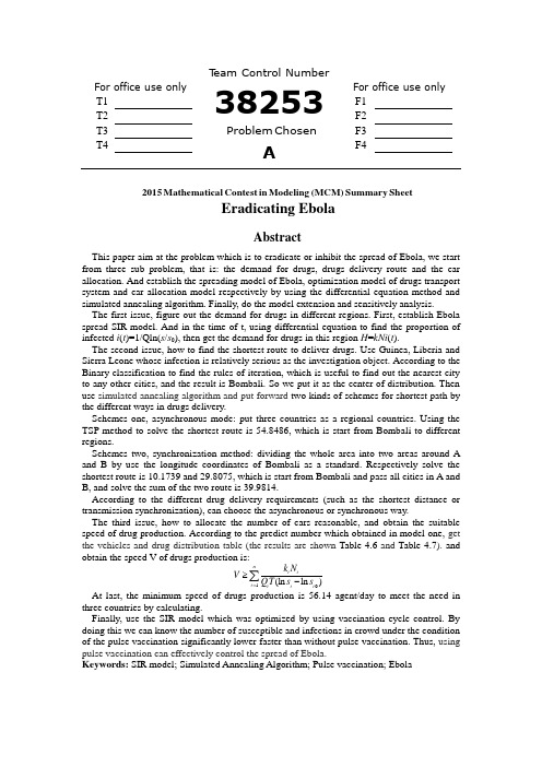
T eam Control NumberFor office use only38253For office use onlyT1F1 T2 F2 T3 Problem ChosenF3 T4 AF42015 Mathematical Contest in Modeling (MCM) Summary SheetEradicating EbolaAbstractThis paper aim at the problem which is to eradicate or inhibit the spread of Ebola, we start from three sub problem, that is: the demand for drugs, drugs delivery route and the car allocation. And establish the spreading model of Ebola, optimization model of drugs transport system and car allocation model respectively by using the differential equation method and simulated annealing algorithm. Finally, do the model extension and sensitively analysis.The first issue, figure out the demand for drugs in different regions. First, establish Ebola spread SIR model. And in the time of t, using differential equation to find the proportion of infected i (t )=1/Qln(s /s 0), then get the demand for drugs in this region H =kNi (t ).The second issue, how to find the shortest route to deliver drugs. Use Guinea, Liberia and Sierra Leone whose infection is relatively serious as the investigation object. According to the Binary classification to find the rules of iteration, which is useful to find out the nearest city to any other cities, and the result is Bombali. So we put it as the center of distribution. Then use simulated annealing algorithm and put forward two kinds of schemes for shortest path by the different ways in drugs delivery.Schemes one, asynchronous mode: put three countries as a regional countries. Using the TSP method to solve the shortest route is 54.8486, which is start from Bombali to different regions.Schemes two, synchronization method: dividing the whole area into two areas around A and B by use the longitude coordinates of Bombali as a standard. Respectively solve the shortest route is 10.1739 and 29.8075, which is start from Bombali and pass all cities in A and B, and solve the sum of the two route is 39.9814.According to the different drug delivery requirements (such as the shortest distance or transmission synchronization), can choose the asynchronous or synchronous way.The third issue, how to allocate the number of cars reasonable, and obtain the suitable speed of drug production. According to the predict number which obtained in model one, get the vehicles and drug distribution table (the results are shown Table 4.6 and Table 4.7). and obtain the speed V of drugs production is:10(ln ln )ni ii i i i k N V Q T s s =≥-∑At last, the minimum speed of drugs production is 56.14 agent/day to meet the need in three countries by calculating.Finally, use the SIR model which was optimized by using vaccination cycle control. By doing this we can know the number of susceptible and infections in crowd under the condition of the pulse vaccination significantly lower faster than without pulse vaccination. Thus, using pulse vaccination can effectively control the spread of Ebola.Keywords: SIR model; Simulated Annealing Algorithm; Pulse vaccination; EbolaEradicating EbolaContent1 Restatement of the Problem (1)1.1 Introduction (1)1.2 The Problem (1)2 General Assumptions (1)3 Variables and Abbreviations (2)4 Modeling and Solving (2)4.1 Model I (2)4.1.1 Analysis of the Problem (2)4.1.2 Model Design (2)4.2 Model II (6)4.2.1 Analysis of the Problem (6)4.2.2 Model Design (6)4.3 Model Ⅲ (8)4.3.1 Analysis of the Problem (8)4.3.2 Model Design (9)4.4 Extent our models (11)5 Sensitivity Analysis (14)5.1 Effect of Daily Contact Rate (14)5.2 Effect of inoculation rate (14)6 Model Analysis (15)6.1 The Advantages of Model (15)6.2 The Disadvantages of Model (15)7 Non-technical Explanation (16)References (18)1Restatement of the Problem1.1IntroductionEbola virus is a very rare kind of virus. It can cause humans and primates produce Ebola hemorrhagic fever virus, and has a high mortality rate. The largest and most complex Ebola outbreak appeared in the West African country in 2014. This outbreak occurred in guinea first, then through various ways to countries such as Sierra Leone, Liberia, Nigeria and Senegal. The number of cases and deaths, which occurred in this outbreak, is more than the sum of all the other epidemic. And outbreak continued to spread between countries. On August 8, 2014, the general-director of the world health organization announced the outbreak of public health emergency of international concern.In this paper, a realistic and reasonable mathematic model, which considers several aspects such as vaccine manufacturing and drug delivery, has been built.Then optimizing the model to eliminate or suppress the harm done by the Ebola virus.1.2The ProblemEstablishing a model to solve the spread of the disease, amount of drugs needed, possible feasible transportation system, transporting position, the speed of a vaccine or drug manufacturing and any other key factor. Thus, we decompose the problem into three sub-problem, modeling and finding the optimization method to face the Ebola virus.♦Building a model, which can solve the spread of the disease and the demand for drugs.♦Building a model to find the best solution.♦Using the goal programming to solve the problems of production and distribution and optimization of other factors..2General AssumptionsTo simplify the problem, we make the following basic assumptions, each of which is properly justified.♦Our assumptions is reasonable and effective.♦Vehicles only run in the path which we have simulated♦This assumption greatly simplify our model and allow us to focus on the shortest path.♦We consider the model that are enclosed.♦People who recovered, will not infected again, and exit the transmission system3Variables and AbbreviationsThe variables and abbreviations used in this paper are listed in Table 3.1.Table 3.1 Assuming variableSymbol DefinitionS the number of susceptible peopleI the number of infected personsR the number of recoveredT a vaccine or drug production cycleH the amount of drugs needed by RegionA a cycle of a vaccine or drug productionL drug reserve area to the shortest path to all affected areasV speed of vaccine or pharmaceutical productionV’vehicle speedλrate of patient contact per dayμday cure rate per dayαn rights of those infected regions weight4Modeling and Solving4.1Model I4.1.1Analysis of the ProblemAccording to the literature that different types of virus has its own different propagation process characteristics, we do not analyze the spread of viruses from a medical point of view, but from the general to analyze the propagation mechanism. So we have to analyze the spread of the Ebola virus and the requirements of drugs through the SIR[1] model.4.1.2Model DesignIn the dynamics of infectious diseases, the main follow Kermack and McKendrick SIR epidemic model which the dynamics of the established method in 1927. SIR model until now is still widely used and continue to develop. SIR model of the total population is divided into the following three categories: susceptibles, the ratio of the number denoted by s(t), at time t is not likely to be infected, but the number of infectious diseases such proportion of the total; infectives, the ratio of the number denoted by i(t), at time t become a patient has been infected and has the proportion of the total number of contagious; recovered, the ratio of the number denoted by r(t), expressed the number of those infected at time t removed from the total proportion (ie, it has quit infected systems). Assuming a total population of N(t), then there are N(t) = s(t) + i(t) + r(t).SIR model is established based on the following two assumptions:In the investigated region-wide spread of the disease is not considered during the births, deaths, population mobility and other dynamic factors. Total population N(t) remainunchanged, the population remains a constant N.The patients’ contact rate (the average number of effective contacts per patient per day) is constant λ, the cure rate (patients be cured proportion of the total number of patients a day) is a constant μ, clearly the average infectious period of 1/μ, infectious period contact number for Q = λ/μ.In the model based on the assumption that we develop a susceptible person to recover fromthe sick person in the process, such as Figure 4.1:Figure 4.1 SIR the model flowchartSIR basis differential equation model can be expressed as:disi i dt dssi dt dri dt λμλμ⎧=-⎪⎪⎪=-⎨⎪⎪=⎪⎩(5.1)But it can see that s(t), i(t) is more difficult to solve, so we use the numerical calculations to esti mate general variation. Assuming λ = 1, μ = 0.3, i(0) = 0.02, s(0) = 0.98 (at the initial time), then we borrow MATLAB software programming to get results. And according to Table 4.1 analyzed i(t), s(t) of the general variation.Figure4.2 s(t),i(t)The patient scale map Figure 4.3 i ~s Phase track diagramFrom Table 4.1 and Figure4.2, we can see that i(t) increased from the initial value to about t = 7(maximum), and then began to decrease.Based on the calculating the numerical and graphical observation, use of phase trajectories discussed i(t), s(t) in nature. Here i ~ s plane is phase plane , the domain (s, i)∈D in phase plane for:{}(,)0,0,1D s i s i s i =≥≥+≤(5.2)According to equation (5.1) and con tact number of the infectious period Q = λ / μ, we can eliminate dt, get:0011(1)(1)i s i s s sdi ds di ds Q Q =-⋅⇒=-⋅⎰⎰(5.3)Calculated using integral characteristics:0001()()ln si t s i s Q s =+-=(5.4)Curve in the domain of definition, equation(5.3) is a phase trajectory.According to equation(5.1) and equation(5.3), have to analyze the changes. If and only if the patient i(t) for some period of growth, it think that in the spread of infectious diseases , then 1/Q is a threshold. If s 0> 1/Q, infectious diseases will spread , and reduce infectious period the number of contacts with Q, namely raising the threshold 1/Q and will make s 0≤1/Q, then it will not spread diseases.And we note that Q = λ/μ in the formula, the higher the level of people's health, the smaller patients’ contact rate; the higher the level of medical, the cure rate is larger and the smaller Q. Therefore, to improve the level of hygiene and medical help to control the spread of infectious diseases. Of course, can also herd immunity and prevention, to reduce s 0.In the process, we analyzed the spread of the disease, then we are going to discuss the amount of medication needed.According to equation(5.4), you can get i(t) values, we can calculate the number of people infected with the disease who I was:()()I i t N t =⋅(5.5)And the amount of drug required, we can be expressed as: H kI =(k is a constant, w> 0)If k> 0, it indicates that the number of infections is still rising, measures to control the virus also needs to be strengthened, and the amount of drugs is a growing demand mode until fluctuation; if k≤0, it means reducing the number of people infected, the virus the measure is better, and the dose of demand is also gradually reduced.According to the data provided by the WHO, we can get the number of infections various,which areas before January 30, 2015. see Table 4.2:Table 4.2 As the number of infections January 30, 2015Region Number Proportion Region Number ProportionNzerekore 2 0.0045 Koinadugu 1 0.0022Macenta 1 0.0022 Kambia 25 0.0558Kissdougou 1 0.0022 Western Urban 105 0.2344Kankan 1 0.0022 Western Rural 64 0.1429Faranah 4 0.0089 Mali 1 0.0022Kono 28 0.0625 Boffa 4 0.0089Bo 6 0.0134 Dubreka 11 0.0246Kenema 2 0.0045 Kindia 2 0.0045Moyamba 8 0.0179 Coyah 11 0.0246Port Loko 78 0.1741 Forecariah 24 0.0536Tonkolili 18 0.0402 Conakry 20 0.0446Bombal 18 0.0402 Montserrado 13 0.029Based on the latest data Ebola virus infections in January 2015, and the regional population and the associated parameter value Ebola assumptions, the model has been solved to a time t proportion of those infected i(t) = 1/Q ln (s/s0), using MATLAB software, we have predict the number of infections each region in February, then get a weight value of those infected forecast for each region in February 2015, as can be show Table 4.3.Table 4.3 As the number of infections February 28, 2015Region Number Proportion Region Number ProportionNzerekore 1 0.00233 Koinadugu 8 0.01864Macenta 3 0.00700 Kambia 24 0.05594Kissdougou 2 0.00470 Western Urban 69 0.16083Kankan 1 0.00233 Western Rural 78 0.18182Faranah 2 0.00470 Mali 4 0.00932Kono 22 0.05130 Boffa 2 0.00470Bo 5 0.01166 Dubreka 10 0.02331 Kenema 5 0.01166 Kindia 1 0.00233Moyamba 1 0.00233 Coyah 9 0.020979Port Loko 100 0.23310 Forecariah 20 0.046620Tonkolili 12 0.02797 Conakry 18 0.041968Bombal 23 0.05361 Montserrado 9 0.020979From Table 4.2 can be known, According to the number of cases of expression,we made a rough prediction that Ebola outbreak in February. it’s provide a reference for the production of vaccines and drugs. Indeed, it have provide a theoretical basis for the relevant departments which take appropriate precautions.4.2Model II4.2.1Analysis of the ProblemBased on the model I, we obtained the equation expression of disease transmission speed and number of drugs. However, in addition to these two factors, we should also consider how to transport drugs to the demanded area quickly and effectively. Thus, it is very important to develop a good transportation system, which can greatly improve the efficiency of drug transport and reduce the cost.4.2.2Model DesignBy searching on Wikipedia, we obtain cities which have erupted Ebola, and the latitude and longitude coordinates[2]. The results are shown in Table 4.4We get the best point, which is Bombali by programming. So, we assume it as the city which produces drugs.Because these cities are breaking points, both as a place of delivery. In order to find out the optimal path, we make following assumptions:♦The demand for each city is same♦The quantity of vehicles can meet the demand of transport♦Vehicles only run in the path which we have simulated4.2.2.1SA modelSA[3] is a random algorithm which is established by imitating metal annealing principle. It can be implemented in large rough search and local fine search by controlling the changes of temperature.Basic principle of SA:♦First, generated initial solution x0 randomly, and make it as the current best solution xopt. Then calculate the value of objective function f (xopt).♦Second, make a random fluctuation on the current solution. Then calculate the value of the new objective function f (x).♦Calculating and judgingΔf = f(x) - f(xopt).IfΔf >0, accept it as the current best solution;Otherwise, accept it in the form of probability P.The calculation method of P is:10=exp[(()())]0opt i f P f x f x f ≤⎧⎨-->⎩ (5.6)In this chapter, the SA algorithm is extended by selecting Bombali as a starting point to solve the optimal path. In the extended SA algorithm.we exploits the exponential cooling strategies and controls the change of temperature, namely10k i T Apha T -=⨯(5.7)Where T i is current controlled temperature, T 0 is the initial temperature, Apha is temperature reduction coefficient, k is the iterations.Solving the initial temperature 0T by means of random iterative and setting Apha = 0.9, the results are shown in Figure 4.4Longitude coordinates of citiesP a r a l l e l v a l u e o f c i t i e sthe total distance:54.8486Figure 4.4 Path graphThe value of the shortest total distance y is 54.8486 The shortest path is presented as follow:Bombali →Tonkolili →Nzerekore →Moyamba →Kambia →Port Loko →Coyah →Mali →Bo →Kindia →Western Urban →Kono →Dubreka →Faranah →Western Rural →Kenema →Kiss-dou gou →Kankan →Forecariah →Boffa →Macenta →Conakry →Montserrado →Koinadugu → Bombali4.2.2.2 SA model refinementSA model got all the shortest path problem of the city, but transport route is single and the efficiency is not high. So we use the longitude coordinates of Bombali as the basis to divide these cities into two parts. Urban classification is shown inTable 4.5, then simulate respectively.Table 4.5 The divided city distributionClassify CitiesLeft half Conakry, Moyamba, Port Loko, Kambia, Western Urban, Western Rural, Boffa, Dubreka, Kindia, Coyah, Forecariah, Bombali.Right halfMontserrado, Nzerekore, Macenta, Kissdougou, Kankan, Faranah, Kono, Bo, Kenema, Tonkolili, Koinadugu, Mali, Bombali .Bombali appears twice, because it is the starting point.After the algorithm simulation result is shown in Figure4.5 and Figure 4.6:Longitude coordinates of citiesP a r a l l e l v a l u e o f c i t i e sLongitude coordinates of citiesP a r a l l e l v a l u e o f c i t i e sthe total distance:28.2716Figure4.5 Left half Figure 4.6 Right halfThe path of left half :Bombali →Port Loko →Boffa →Forecariah →Dubreka →Moyamba →Kindia →Coyah →West e-rnRural →Conakry →Kambia →Western Urban →Bombali The path of right half :Bombali →Kenema →Faranah →Mali →Nzerekore →Bo →Kissdougou →Kankan →Koinadu gu →Kono →Tonkolili →Montserrado →Macenta →Bombali The total distance is:L=10.1739+29.8075=39.9814.It is smaller than the answer before, the transport time is reduced and the efficiency of transportation is improved.4.3 Model Ⅲ4.3.1 Analysis of the ProblemAccording to the above analysis of the first model and the second model, we can learn something about the spreading of Ebola, then finding the shortest path to transport medicines or vaccines. On the basis of the spreading of Ebola, we can know the numbers of illness with Ebola, then, get the quantity demanded of illness. According to the city distribution of infected zone, we find the shortest path to transport medicines, as well as ensure the shortest transporting route.After comprehending the demand for vaccine in infected zones and its the shortest transporting route, the next problem we think about is how to transport the vaccines or drugs from storage zone to infected zone using the maximum efficiency. Besides, we also need to consider whether the production speed can keep up with the demand for drugs and delivery speed. That is to say, the quantity of medicine production must be greater than or equal to the demand for drugs. Only in this method can we give sufficient vaccines or drugs to infected zones by using the fastest speed to control the spread of Ebola. 4.3.2 Model DesignIn the second model, we consider the shortest path and find the shortest path to all infected zones, then get its occurrence of distance. Getting the basic solve of the first model and the second model, the drugs or vaccines transport system can allot cars for infected zones judging by the weight of the numbers of infections in different cities. hypothesis :♦ All allocation cars are the same vehicle size, moreover, have sufficient cars. That is to say, the quantity of vaccines or drugs in all cars is equal.♦ All delivery routes will not block up, and the cars will not break down. That is to say, all allocation cars can reach the infected area on time.♦ In order to avoid Ebola propagate to other place, this area should be isolated immediately once this area burst Ebola.♦ The car allocation in different regions can match up with the pharmaceutical demand in different regions. That is to say, they are positively related♦ By looking for date, we can get the number of infections in different regions :I1,I2,I3….In, then get the weight of the number of infections in different regions:11,2,3nn nnn I n Iα===∑(5.8)The pharmaceutical demand in different regions is:1,2,3n n H C n α==(5.9)C is the total quantity of car ,αn is the weight of the number of infections in different regions.According to the hypothesis, we can know that the pharmaceutical demand in each infected zone is directly related to the car allocation, so, we allot all cars in the light of weight. That is to say, the bigger weight can get more cars, the smaller weight will get less cars. Thus, we not only can save time, but also cost.According to the above analysis, we can know that the model also should meet the follow conditions:123'n A H H H H L T V ≥++++⎧⎪⎨≤⎪⎩(5.10)H n is the pharmaceutical demand in different regions, V 'is vehicle speed, T is theproduction cycle of vaccines or drugs. According to the model I solving scheme, we can get the proportion of infected is i(t)=1/Qln(s/s 0)in t time, At the same time the region's demand for drugs is H=kNi(t), Drug production speed need to meet :10(ln ln )ni ii i i i k N V QT s s =≥-∑(5.11)We seek the latest date information from WTO official website [4], and get the new casedistribution graphs of Guinea 、Sierra Leone 、Liberia .You can see on Figure 4.7Figure 4.7 Geographical distribution of new and total confirmed casesWe can get the number of infections about 24 cities in infected zones from the diagram [5], then figure out the weight of infection numbers in different regions and clear up these dates. You can see on the Table 4.1.According to the model I, it have forecast the number of infections in 2015 February, and calculate the number of infections in various regions of the weight, the allocation of all transport vehicles, and have meet the demand for drugs in February at epidemic area. so, according to the predicted values, We can get the drug distribution table show in Table 4.6 and vehicle allocation table show in Table 4.7.the future of the epidemic and how to reasonable distribution of drugs,.According to the above model analysis, after ensuring the demand for vaccines and medicines in different regions and the shortest transport route, and on the double bind of medicine production speed and medicine delivery speed. we have a discussion ,then get the car allocation in different regions to make sure the medicines or vaccines reach the infected zones by using the fastest speed. So, we can remit current epidemic situation of Ebola.4.4 Extent our modelsIn the model I, we have studied the classical SIR epidemic model, then we have an improved in the model I, the improved model is:()()()()()()()()dSN I S t dt dIS t I t I t dt dRI t R t dt λβλβλμμλ⎧=-+⎪⎪⎪=-+⎨⎪⎪=-⎪⎩(5.12)In the infectious disease model, We've added the μto the population birth rate and natural mortality, ‘β’is the coefficient of the spread of the disease, ‘N’ is the number of species number. In this model assumes that there is no population move out and the death due to illness, the number of population is constant.As mentioned above, the ‘I’ is the number of infected patients, if the ‘S’ ‘I’ ‘R’ have given the initialvalue, By solving the differential equations(5.12), can get the value of ‘I(t)’ at a certain moment. For this model, we expect the people infected can stable at a low level, this means that the spread of infectious diseases has been effectively controlled. Analyzed the infectious disease model, if we want to control effectively to ‘I’, should decrease the coefficient of the spread of the disease β, and improve disease recovery rate λ, In terms of emergency rescue, it’s should ensure that there are have adequate relief drug to patients in emergency treatment, and make the probability of recovery to increase, then , it can control effectively to the increase of ‘I’.At the beginning of the outbreak of infectious diseases, when it ’s have a pulse vaccination for the population cycle T, the spread of the corresponding SIR epidemic model [6] is shown in Figure 4.8, Propagation model expressed in equation (4.13).S λI λRλFigure 4.8 The flow chart of pulse SIR1()()()()()()()()()(1)()()()0,1,2()()()nn nn dSN I S t dt dI S t I t I t t tdt dR I t R t t t T dtS t p S t I t I t t t n R t R t pS t λβλβλμμλ+----⎧=-+⎪⎪⎪=-+≠⎪⎪⎨=-=+⎪⎪=-⎪⎪===⎪=+⎩(5.13)P is vaccination rate.Impulsive vaccination is different from traditional large-scale disposable vaccination, it can ensure to make an effective control by using the spread of lower vaccination rate. We can obtain something from the analysis of the first model that i(t) is the function which increase first and then decrease with the time. Thus, the population infected will tend to zero ultimately. If 0dIdt <, then the critical value of c S is:()(1)(1)T c TT p e pTS T p e λλλγλλβλ+--+=>-+ (5.14)Then the critical value of c p is :()(1)()(1)T c T T e p T e λλλλμβμβλμβ+--=--+- (5.15)We can know that, if the vaccination rate p>p c , system can obtain a stable disease-free periodic solution.When the infectious disease, which is described at model(5.12), burst out at one region, we should firstly know the demand for vaccine in different rescue cycle area before doing vaccinate to the infected populations. On account of epidemical diffusion law that indicated by SIR model(5.13), which possessing the pulse vaccination, we use the following form of demand forecasting that change over time.()k k D pS T -=(5.16)We can know something from the second model that we divide the whole infected zone into two regions. The two regions are assumed to be A and B. There is a stockpile around A and B. Known about the above information, we use the suggested model to do car allocation for A and B.Given the parameters in Ebola spread model(5.13) and its initial value, as shown in the Table 4.8 and Table 4.9. If the pulse vaccination cycle T=50, we use MATLAB programming to figure out the arithmetic solution of Ebola spread model (5.8) and model(5.9), as shown in the follow form:Table 4.8 Infectious disease model parametersParameter λ β μ p T Numerical0.000060.000020.0080.150Table 4.9 A and B area initial values i r Infected area A 830 370 0 Infected area B92278daysn u m b e r sthe SIR model with pulse vaccination in the demand point Adaysn u m b e r sthe SIR model without pulse vaccination in the demand point A(a) (b)daysn u m b e r sthe SIR model with pulse vaccination in the demand point Bdaysn u m b e r sthe SIR model without pulse vaccination in the demand point B(c) (d)Figure 4.9 Numerical solution of diffusion model SIR diseaseCompare Figure 4.9(a) with Figure 4.9(b), we can see that infected people and vulnerable people are going down faster under the circumstance of pulse vaccination. The same circumstance can be seen in the comparison of Figure 4.9(c) and Figure 4.9(d), it indicate that the pulse vaccination can control the spread of Ebola more effective. Because of this, we use the pulse vaccination to make our model solve the spread of Ebola preferably.5 Sensitivity Analysis5.1 Effect of Daily Contact RateIn model Ⅰ, we get the variation of function i (t ) and s (t ) by assuming variable value. So further discuss the value of λ is 2 or 3 whether impact on the result.Based on MATLAB software programming, can get the graphics when λ=2 or λ=3.daysn u m b e r sThe rate of healthy people and patientsdaysn u m b e r sThe rate of healthy people and patientsFigure 5.1 λ=2 or λ=3Conclusion:♦ Through comparing with Figure 4.2 ( λ=1 ) in model Ⅰ, it can be seen that the growth of the I (t) section is slightly reduced.♦ Observe the Figure 5.1, you can see λ=2 or λ=3 graphics haven't changed much5.2 Effect of inoculation rateIn the model Ⅲ, we have introduced the method of pulse vaccination. At the same time drew a conclusion that pulse vaccination can effectively control the spread of the virus.。
MCM品牌介绍PPT精选文档

MCM
MCM品牌1976年创始于德国的慕尼黑,创始人是 好莱坞影星——Michael Cromer 字母“MCM”分
别代表Mode(时尚)、Creation(创造力)、 Munich(慕尼黑)。MCM品牌的产品线以服装、服饰 和皮具为主。 原产地:德国 MCM总裁兼主席:金圣珠(SungJoo Kim) (2005年, 韩国女商人Sung-joo Kim收购了MCM品牌) MCM创意总监:Michael Michalsky(迈克尔.米夏尔斯 基)
2007年MCM立足于世界时尚中心,进入了一个动态增长的时代。在米 兰时装周之后,MCM同时在美国12个主要城市的Bloomingadales、 Fred Segal、 Intermix以及Harrods百货商店与Selfridges 百货商店 开始出售。作为俄国的第一家,MCM品牌在位于莫斯科的Tsum百货 出售,在雅典也开了一家专卖店,继而11月在泰国的Zen百货出售。继 在伦敦奢侈品林立的Sloane Street 开设的两层楼的精品店之后, MCM将在韩国首尔最奢侈的品牌区Chengdam-Dong 开设全球第一家 五层楼高的旗舰店,它还计划在全世界各个地区如纽约、杜塞尔多夫与 澳门等地开办更多的商店。消费者将可以在纽约The Plaza,印度尼西 亚、新加坡与台湾看到更多的MCM商店
MCM皮具最大的特点是纯手工制作,第二大特点 是每一件产品上有一个铜牌,上面标有独一无二的 编号。只有极少的一些国际大牌,才会在自己的每 一件产品上有一个不同的编码,所以MCM每一件 产品都会像一个艺术品非常的精致、珍贵。
2014 flower boys in paradise系列 该系列灵感来源于关于“理想”
著名欧洲新奢侈时装品牌MCM (Mode Creation Munich) 最初以制作高级旅行皮具起 家。在八十年代品牌的全盛时期,MCM生产包 括手表、珠宝、香水、服装、箱包以及小型皮具 等在内的超过五百款的产品。它时髦、奢侈而实 用的产品非常畅销。如今,MCM承袭其一贯的 款式时尚、品质精良的风格与传统,演变成为全 球的奢侈品牌之一。 设计灵感源自于1968-1978年慕尼黑的建筑、电 影、音乐、艺术、摄影、现代生活方式、时尚、 美态、科技、旅行和灵活性,展现了二十世纪七
- 1、下载文档前请自行甄别文档内容的完整性,平台不提供额外的编辑、内容补充、找答案等附加服务。
- 2、"仅部分预览"的文档,不可在线预览部分如存在完整性等问题,可反馈申请退款(可完整预览的文档不适用该条件!)。
- 3、如文档侵犯您的权益,请联系客服反馈,我们会尽快为您处理(人工客服工作时间:9:00-18:30)。
Number of People Entered Shanghai World Expo Park Abstract:Key words:Contents1. Introduction (3)1.1 Why does toll way collects toll? (3)1.2 Toll modes (3)1.3 Toll collection methods (3)1.4 Annoyance in toll plazas (3)1.5 The origin of the toll way problem (3)1.6 Queuing theory (4)2. The Description of Problem (5)2.1 How do we approximate the whole course of paying toll? (5)2.2 How do we define the optimal configuration? (5)2.2.1 From the perspective of motorist (5)2.2.2 From the perspective of the toll plaza (6)2.2.3 Compromise (6)2.3 Overall optimization and local optimization (6)2.4 The differences in weights and sizes of vehicles (7)2.5 What if there is no data available? (7)3. Models (7)3.1 Basic Model (7)3.1.1 Symbols and Definitions (7)3.1.2 Assumptions (8)3.1.3 The Foundation of Model (9)3.1.4 Solution and Result (11)3.1.5 Analysis of the Result (11)3.1.6 Strength and Weakness (13)3.2 Improved Model (14)3.2.1 Extra Symbols (14)3.2.2 Additional Assumptions (14)3.2.3 The Foundation of Model (14)3.2.4 Solution and Result (15)3.2.5 Analysis of the Result (18)3.2.6 Strength and Weakness (19)4. Conclusions (19)4.1 Conclusions of the problem (19)4.2 Methods used in our models (19)4.3 Application of our models (19)5. Future Work (19)5.1 Another model (19)5.2 Another layout of toll plaza (23)5.3 The newly- adopted charging methods (23)6.References (23)7.Appendix (23)Programs and codes (24)I. IntroductionIn order to indicate the origin of the toll way problems, the following background is worth mentioning.1.11.21.31.41.51.6II. The Description of the Problem2.1 How do we approximate the whole course of paying toll?●●●●2.2 How do we define the optimal configuration?1) From the perspective of motorist:2) From the perspective of the toll plaza:3) Compromise:2.3 The local optimization and the overall optimization●●●Virtually:2.4 The differences in weights and sizes of vehicles2.5 What if there is no data available?III. Models3.1 Basic Model3.1.1 Terms, Definitions and SymbolsThe signs and definitions are mostly generated from queuing theory.●●●●●3.1.2 Assumptions●●●●●3.1.3 The Foundation of Model1) The utility function●The cost of toll plaza:●The loss of motorist:●The weight of each aspect:●Compromise:2) The integer programmingAccording to queuing theory, we can calculate the statistical properties as follows.3)The overall optimization and the local optimization●The overall optimization:●The local optimization:●The optimal number of tollbooths:3.1.4 Solution and Result1) The solution of the integer programming:2) Results:3.1.5 Analysis of the Result●Local optimization and overall optimization:●Sensitivity: The result is quite sensitive to the change of the threeparameters●Trend:●Comparison:3.1.6 Strength and Weakness●Strength: In despite of this, the model has proved that . Moreover, wehave drawn some useful conclusions about . T he model is fit for, such as●Weakness: This model just applies to . As we have stated, .That’sjust what we should do in the improved model.3.2 Improved Model3.2.1 Extra SymbolsSigns and definitions indicated above are still valid. Here are some extra signs and definitions.●●●●3.2.2 Additional Assumptions●●●Assumptions concerning the anterior process are the same as the Basic Model.3.2.3 The Foundation of Model1) How do we determine the optimal number?As we have concluded from the Basic Model,3.2.4 Solution and Result1) Simulation algorithmBased on the analysis above, we design our simulation arithmetic as follows.●Step1:●Step2:●Step3:●Step4:●Step5:●Step6:●Step7:●Step8:●Step9:2) Flow chartThe figure below is the flow chart of the simulation.3) Solution3.2.5 Analysis of the Result3.2.6 Strength and Weakness●Strength: The Improved Model aims to make up for the neglect of .The result seems to declare that this model is more reasonable than the Basic Model and much more effective than the existing design.●Weakness: . Thus the model is still an approximate on a large scale. Thishas doomed to limit the applications of it.IV. Conclusions4.1 Conclusions of the problem●●●4.2 Methods used in our models●●●4.3 Applications of our models●●●V. Future Work5.1 Another model5.1.1The limitations of queuing theory 5.1.25.1.35.1.41)●●●●2)●●●3)●●●4)5.2 Another layout of toll plaza5.3 The newly- adopted charging methodsVI. References[1][2][3][4]VII. Appendix。