2012年美国数学建模icm翻译
数学建模美赛经验

23
我们的美赛——分析理解问题
原题给了几个参考文献,但是页数太多,只要关注主要的概念就行。 题目中给的数据来源比较有用。
24
我们的美赛——分析理解问题
为了理解,题目中提到的可持续发展的概念。 我去知网找了中文论文,看了20-30篇文章。最后选出3篇参考。 论文的搜索方法:
知网及其他搜索引擎的检索表达式;通过被引用次数排序选取重要论文;通过参考 文献来寻找节点论文。
9
数学建模的必备能力——模型运用和实现
推荐资料
《数学建模算法与程序》 主编:司守奎 如右图,这本书里面有基本的数学模型和matlab的代码实现。
10
数学建模的必备能力——结果表现
高超的画图技能
11
数学建模的必备能力——结果分析及问题拓 展
1、是否解决了问题。 将模型预测和评价的结果与实际结果相对比。
2、D题交叉学科,更多涉及数据处理。更适合现学现卖。
3、要求20页以内,相对容易完成。
18
我们的美赛——分析理解问题
Problem D - Is it sustainable?
19
我们的美赛——分析理解问题
20
我们的美赛——分析理解问题
21
我们的美赛——分析理解问题
22
我们的美赛——分析理解问题
14
获奖
根据评审流程,摘要写的好,排版没问题,就可以拿二等奖。 多读英文论文,保证论文语法和内容填充的质量。 切合问题的、逻辑严谨的数学模型。 根据自身队伍特点扬长避短选择题目,并且发挥自己的优势把问题引导到自己擅长 的领域。 节约比赛中的时间,能事先做好的工作就不要在比赛中做。
美国大学生数学建模竞赛数据及评阅分析_吴孟达
给出了 MCM 和ICM 中国队和美国队参赛队数的变化。
图1分析:
● MCM 参赛队数10年间年均增长25%,近5年年均增长33.8%,增速明显加快。
● 美国参赛队增长不明显,增长队数主要来自于中国参赛队的增长。
收 稿 日 期 :2012-11-09 通 讯 作 者 :吴 孟 达 ,E-mail:mdwu@nudtwmd.com
摘 要:统计了美国大学生数学建模竞赛近十年的参赛数据,对其评阅过程进行 了 分 析,得 出 了 一 些 有 参 考 价 值 的 结论。 关 键 词 :美 国 大 学 生 数 学 建 模 竞 赛 ;中 国 大 学 生 数 学 建 模 竞 赛 ;获 奖 比 例 ;评 阅 过 程
中 图 分 类 号 :O29 文 献 标 志 码 :A 文 章 编 号 :2095-3070(2012)04-0075-04
3 26 1 273 2 373 687 1 854 332 1 282 342 849 357 627 235 466 194 389 125 295 103 195 105
11(3) 7(6) 8(3) 6(4) 9(2) 4(2) 9(1) 2(1) 9(0) 3(2)
图2 ICM 参赛队数变化图 图3 MCM 获奖比例 图4 ICM 获奖比例
2 评 阅 过 程 分 析
据 美 赛 “评 委 评 论 ”介 绍 ,美 赛 评 阅 过 程 大 致 分 为 三 轮 。 第一轮可以称为“淘汰轮(the Triage Round)”。此轮评阅主要以摘要信息以及论文整体结构为 评 判 依 据 ,时 间 大 约 是 5~10 分 钟 。 每 个 评 委 以 “通 过 ”、“不 通 过 ”计 分 ,事 先 应 当 设 置 有 大 致 的 “通 过 ”比 例 (此 轮 与 国内研赛的网评阶段相类似)。当两位 评 委 意 见 不 一 致 时 可 以 协 商 达 成 一 致 意 见,如 果 仍 不 能 达 成 一 致 意 见 ,则 请 第 三 位 评 委 评 阅 。 有 “评 论 ”介 绍 说 ,这 一 轮 的 淘 汰 率 大 约 为 45% ,通 过 这 一 轮 评 审 的 参 赛 队 大 约 有 80% 的 获 奖 概 率 。 关 于 如 何 通 过 这 一 轮 评 审 ,评 委 给 出 的 建 议 是 : 1)摘 要 至 关 重 要 ,必 须 清 晰 且 信 息 量 充 分 。 评 委 关 心 的 是 你 对 问 题 的 理 解 是 否 准 确 ,你 建 立 的 模 型 及 使 用的方法是否恰当,以及根据你所建模型得到的主要结果和主要结论是否合理 。 过 于 冗 长 的 技 术 性 描 述 将 · 76 ·
美国大学生数学建模竞赛翻译必备知识
Aabsolute value 绝对值accept 接受acceptable region 接受域additivity 可加性adjusted 调整的alternative hypothesis 对立假设analysis 分析analysis of covariance 协方差分析analysis of variance 方差分析arithmetic mean 算术平均值association 相关性assumption 假设assumption checking 假设检验availability 有效度average 均值Bbalanced 平衡的band 带宽bar chart 条形图beta-distribution 贝塔分布between groups 组间的bias 偏倚binomial distribution 二项分布binomial test 二项检验Ccalculate 计算case 个案category 类别center of gravity 重心central tendency 中心趋势chi-square distribution 卡方分布chi-square test 卡方检验classify 分类cluster analysis 聚类分析coefficient 系数coefficient of correlation 相关系数collinearity 共线性column 列compare 比较comparison 对照components 构成,分量compound 复合的confidence interval 置信区间consistency 一致性constant 常数continuous variable 连续变量control charts 控制图correlation 相关covariance 协方差covariance matrix 协方差矩阵critical point 临界点critical value 临界值crosstab 列联表cubic 三次的,立方的cubic term 三次项cumulative distributionfunction 累加分布函数curve estimation 曲线估计Ddata 数据default 默认的definition 定义deleted residual 剔除残差density function 密度函数dependent variable 因变量description 描述design of experiment 试验设计deviations 差异df.(degree of freedom) 自由度diagnostic 诊断dimension 维discrete variable 离散变量discriminant function 判别函数discriminatory analysis 判别分析distance 距离distribution 分布D-optimal design D-优化设计Eeaqual 相等effects of interaction 交互效应efficiency 有效性eigenvalue 特征值equal size 等含量equation 方程error 误差estimate 估计estimation of parameters参数估计estimations 估计量evaluate 衡量exact value 精确值expectation 期望expected value 期望值exponential 指数的exponential distributon 指数分布extreme value 极值Ffactor 因素,因子factor analysis 因子分析factor score 因子得分factorial designs 析因设计factorial experiment 析因试验fit 拟合fitted line 拟合线fitted value 拟合值fixed model 固定模型fixed variable 固定变量fractional factorial design部分析因设计frequency 频数F-test F检验full factorial design 完全析因设计function 函数Ggamma distribution 伽玛分布geometric mean 几何均值group 组Hharmomic mean 调和均值heterogeneity 不齐性histogram 直方图homogeneity 齐性homogeneity of variance 方差齐性hypothesis 假设hypothesis test 假设检验Iindependence 独立independent variable 自变量independent-samples 独立样本index 指数index of correlation 相关指数interaction 交互作用interclass correlation 组内相关interval estimate 区间估计intraclass correlation 组间相关inverse 倒数的iterate 迭代Kkernal 核Kolmogorov-Smirnov test 柯尔莫哥洛夫-斯米诺夫检验kurtosis 峰度Llarge sample problem 大样本问题layer 层least-significant difference 最小显著差数least-square estimation 最小二乘估计least-square method 最小二乘法level 水平level of significance 显著性水平leverage value 中心化杠杆值life 寿命life test 寿命试验likelihood function 似然函数likelihood ratio test 似然比检验linear 线性的linear estimator 线性估计linear model 线性模型linear regression 线性回归linear relation 线性关系linear term 线性项logarithmic 对数的logarithms 对数logistic 逻辑的lost function 损失函数Mmain effect 主效应matrix 矩阵maximum 最大值maximum likelihoodestimation 极大似然估计mean squareddeviation(MSD) 均方差mean sum of square 均方和measure 衡量media 中位数M-estimator M估计minimum 最小值missing values 缺失值mixed model 混合模型mode 众数model 模型Monte Carle method 蒙特卡罗法moving average 移动平均值multicollinearity 多元共线性multiple comparison 多重比较multiple correlation 多重相关multiple correlationcoefficient 复相关系数multiple correlationcoefficient 多元相关系数multiple regression analysis多元回归分析multiple regressionequation 多元回归方程multiple response 多响应multivariate analysis 多元分析Nnegative relationship 负相关nonadditively 不可加性nonlinear 非线性nonlinear regression 非线性回归noparametric tests 非参数检验normal distribution 正态分布null hypothesis 零假设number of cases 个案数Oone-sample 单样本one-tailed test 单侧检验one-way ANOVA 单向方差分析one-way classification 单向分类optimal 优化的optimum allocation 最优配制order 排序order statistics 次序统计量origin 原点orthogonal 正交的outliers 异常值Ppaired observations 成对观测数据paired-sample 成对样本parameter 参数parameter estimation 参数估计partial correlation 偏相关partial correlation coefficient 偏相关系数partial regression coefficient 偏回归系数percent 百分数percentiles 百分位数pie chart 饼图point estimate 点估计poisson distribution 泊松分布polynomial curve 多项式曲线polynomial regression 多项式回归polynomials 多项式positive relationship 正相关power 幂P-P plot P-P概率图predict 预测predicted value 预测值prediction intervals 预测区间principal component analysis 主成分分析proability 概率probability density function 概率密度函数probit analysis 概率分析proportion 比例Qqadratic 二次的Q-Q plot Q-Q概率图quadratic term 二次项quality control 质量控制quantitative 数量的,度量的quartiles 四分位数Rrandom 随机的random number 随机数random number 随机数random sampling 随机取样random seed 随机数种子random variable 随机变量randomization 随机化range 极差rank 秩rank correlation 秩相关rank statistic 秩统计量regression analysis 回归分析regression coefficient 回归系数regression line 回归线reject 拒绝rejection region 拒绝域relationship 关系reliability 可靠性repeated 重复的report 报告,报表residual 残差residual sum of squares 剩余平方和response 响应risk function 风险函数robustness 稳健性root mean square 标准差row 行run 游程run test 游程检验Ssample 样本sample size 样本容量sample space 样本空间sampling 取样sampling inspection 抽样检验scatter chart 散点图S-curve S形曲线separately 单独地sets 集合sign test 符号检验significance 显著性significance level 显著性水平significance testing 显著性检验significant 显著的,有效的significant digits 有效数字skewed distribution 偏态分布skewness 偏度small sample problem 小样本问题smooth 平滑sort 排序soruces of variation 方差来源space 空间spread 扩展square 平方standard deviation 标准离差standard error of mean 均值的标准误差standardization 标准化standardize 标准化statistic 统计量statistical quality control 统计质量控制std. residual 标准残差stepwise regressionanalysis 逐步回归stimulus 刺激strong assumption 强假设stud. deleted residual 学生化剔除残差stud. residual 学生化残差subsamples 次级样本sufficient statistic 充分统计量sum 和sum of squares 平方和summary 概括,综述Ttable 表t-distribution t分布test 检验test criterion 检验判据test for linearity 线性检验test of goodness of fit 拟合优度检验test of homogeneity 齐性检验test of independence 独立性检验test rules 检验法则test statistics 检验统计量testing function 检验函数time series 时间序列tolerance limits 容许限total 总共,和transformation 转换treatment 处理trimmed mean 截尾均值true value 真值t-test t检验two-tailed test 双侧检验Uunbalanced 不平衡的unbiased estimation 无偏估计unbiasedness 无偏性uniform distribution 均匀分布Vvalue of estimator 估计值variable 变量variance 方差variance components 方差分量variance ratio 方差比various 不同的vector 向量Wweight 加权,权重weighted average 加权平均值within groups 组内的ZZ score Z分数Ⅱ.2 最优化方法词汇英汉对照表Aactive constraint 活动约束active set method 活动集法analytic gradient 解析梯度approximate 近似arbitrary 强制性的argument 变量attainment factor 达到因子Bbandwidth 带宽be equivalent to 等价于best-fit 最佳拟合bound 边界Ccoefficient 系数complex-value 复数值component 分量constant 常数constrained 有约束的constraint 约束constraint function 约束函数continuous 连续的converge 收敛cubic polynomialinterpolation method三次多项式插值法curve-fitting 曲线拟合Ddata-fitting 数据拟合default 默认的,默认的define 定义diagonal 对角的direct search method 直接搜索法direction of search 搜索方向discontinuous 不连续Eeigenvalue 特征值empty matrix 空矩阵equality 等式exceeded 溢出的Ffeasible 可行的feasible solution 可行解finite-difference 有限差分first-order 一阶GGauss-Newton method 高斯-牛顿法goal attainment problem 目标达到问题gradient 梯度gradient method 梯度法Hhandle 句柄Hessian matrix 海色矩阵Iindependent variables 独立变量inequality 不等式infeasibility 不可行性infeasible 不可行的initial feasible solution 初始可行解initialize 初始化inverse 逆invoke 激活iteration 迭代iteration 迭代JJacobian 雅可比矩阵LLagrange multiplier 拉格朗日乘子large-scale 大型的least square 最小二乘least squares sense 最小二乘意义上的Levenberg-Marquardtmethod列文伯格-马夸尔特法line search 一维搜索linear 线性的linear equality constraints线性等式约束linear programmingproblem 线性规划问题local solution 局部解Mmedium-scale 中型的minimize 最小化mixed quadratic and cubic polynomial interpolation and extrapolation method 混合二次、三次多项式内插、外插法multiobjective 多目标的Nnonlinear 非线性的norm 范数Oobjective function 目标函数observed data 测量数据optimization routine 优化过程optimize 优化optimizer 求解器over-determined system 超定系统Pparameter 参数partial derivatives 偏导数polynomial interpolation method多项式插值法Qquadratic 二次的quadratic interpolation method 二次内插法quadratic programming 二次规划Rreal-value 实数值residuals 残差robust 稳健的robustness 稳健性,鲁棒性Sscalar 标量semi-infinitely problem 半无限问题Sequential Quadratic Programming method序列二次规划法simplex search method 单纯形法solution 解sparse matrix 稀疏矩阵sparsity pattern 稀疏模式sparsity structure 稀疏结构starting point 初始点step length 步长subspace trust regionmethod 子空间置信域法sum-of-squares 平方和symmetric matrix 对称矩阵Ttermination message 终止信息termination tolerance 终止容限the exit condition 退出条件the method of steepestdescent 最速下降法transpose 转置Uunconstrained 无约束的under-determined system负定系统Vvariable 变量vector 矢量Wweighting matrix 加权矩阵Ⅱ.3 样条词汇英汉对照表Aapproximation 逼近array 数组a spline in b-form/b-splineb样条a spline of polynomial piece/ppform spline分段多项式样条Bbivariate spline function 二元样条函数break/breaks 断点Ccoefficient/coefficients 系数cubic interpolation 三次插值/三次内插cubic polynomial 三次多项式cubic smoothing spline 三次平滑样条cubic spline 三次样条cubic spline interpolation三次样条插值/三次样条内插curve 曲线Ddegree of freedom 自由度dimension 维数Eend conditions 约束条件Iinput argument 输入参数interpolation 插值/内插interval 取值区间Kknot/knots 节点Lleast-squaresapproximation 最小二乘拟合Mmultiplicity 重次multivariate function 多元函数Ooptional argument 可选参数order 阶次output argument 输出参数Ppoint/points 数据点Rrational spline 有理样条rounding error 舍入误差(相对误差)Sscalar 标量sequence 数列(数组)spline 样条spline approximation 样条逼近/样条拟合spline function 样条函数spline curve 样条曲线spline interpolation 样条插值/样条内插spline surface 样条曲面smoothing spline 平滑样条Ttolerance 允许精度Uunivariate function 一元函数Vvector 向量Wweight/weights 权重Ⅱ.4 偏微分方程数值解词汇英汉对照表Aabsolute error 绝对误差absolute tolerance 绝对容限adaptive mesh 适应性网格Bboundary condition 边界条件Ccontour plot 等值线图converge 收敛coordinate 坐标系Ddecomposed 分解的decomposed geometry matrix 分解几何矩阵diagonal matrix 对角矩阵Dirichlet boundary conditionsDirichlet边界条件Eeigenvalue 特征值elliptic 椭圆形的error estimate 误差估计exact solution 精确解Ggeneralized Neumann boundary condition推广的Neumann边界条件geometry 几何形状geometry descriptionmatrix 几何描述矩阵geometry matrix 几何矩阵graphical user interface(GUI)图形用户界面Hhyperbolic 双曲线的Iinitial mesh 初始网格Jjiggle 微调LLagrange multipliers 拉格朗日乘子Laplace equation 拉普拉斯方程linear interpolation 线性插值loop 循环Mmachine precision 机器精度mixed boundary condition混合边界条件NNeuman boundarycondition Neuman边界条件node point 节点nonlinear solver 非线性求解器normal vector 法向量PParabolic 抛物线型的partial differential equation偏微分方程plane strain 平面应变plane stress 平面应力Poisson's equation 泊松方程polygon 多边形positive definite 正定Qquality 质量Rrefined triangular mesh 加密的三角形网格relative tolerance 相对容限relative tolerance 相对容限residual 残差residual norm 残差范数Ssingular 奇异的sparce matrix 稀疏矩阵stiffness matrix 刚度矩阵subregion 子域Ttriangular mesh 三角形网格Uundetermined 未定的uniform refinement 均匀加密uniform triangle net 均匀三角形网络Wwave equation 波动方程Algebraic Equation代数方程Elementary Operations-Addition基础混算-加法ElementaryOperations-Subtaction基础混算-减法ElementaryOperations-Multiplication基础混算-乘法Elementary Operations-Division基础混算-除法Elementary Operation基础四则混算Decimal Operations 小数混算Fractional Operations分数混算Convert fractional no. intodecimal no.分数转小数Convert fractional no. intopercentage.分数转百分数Convert decimal no. intopercentage.小数转百分数Convert percentage into decimal no.百分数转小数Percentage百分数Numerals数字符号Common factors and multiples公因子及公倍数Sorting数字排序Area图形面积Perimeter图形周界Change Units : Time单位转换-时间Change Units : Weight 单位转换-重量Change Units :Length单位转换-长度Directed Numbers 有向数Fractional Operations 分数混算Decimal Operations 小数混算Convert fractional no. into decimal no.分数转小数Convert fractional no. into percentage.分数转百分数Convert decimal no. into percentage.小数转百分数Convert percentage into decimal no.百分数转小数Percentage百分数Indices指数Algebraic Substitution 代数代入Polynomials多项式Co-Geometry坐标几何学Solving Linear Equation解一元线性方程Solving Simultaneous Equation解联立方程Slope直线斜率Equation of Straight Line直线方程x-intercept ( Equation of St. Line )直线x轴截距y-intercept ( Equation of St. Line )直线y轴截距Factorization因式分解Quadratic Equation 二次方程x-intercept ( Quadratic Equation )二次曲线x轴截距Geometry几何学Inequalities不等式Rate and Ratio比和比例Bearing方位角Trigonometry三角学Probability概率Statistics-Graph统计学-统计图表Statistics-Measure of centraltendency统计学-量度集中趋势Salary Tax薪俸税Bridging Game汉英对对碰Indices指数Function函数Rate and Ratio比和比例Trigonometry三角学Inequalities不等式Linear Programming线性规划Co-Geometry坐标几何学Slope直线斜率Equation of Straight Line直线方程x-intercept ( Equation of St. Line )直线x轴截距y-intercept ( Equation of St. Line )直线y轴截距Factorization因式分解Quadratic Equation二次方程x-intercept ( Quadratic Equation )二次曲线x轴截距Method of Bisection分半方法Polynomials多项式Probability概率Statistics-Graph统计学-统计图表Statistics-Measure of centraltendency统计学-量度集中趋势Statistics-Measure of dispersion统计学-量度分布Statistics-Normal Distribution统计学-正态分布Surds根式Probability概率Statistics-Measure of dispersion统计学-量度离差Statistics-Normal Distribution统计学-正态分布Statistics-Binomial Distribution统计学Statistics-Poisson Distribution统计学Statistics-Geometric Distribution统计学Co-Geometry坐标几何学Sequence序列十万Hundred thousand三位数3-digit number千Thousand千万Ten million小数Decimal分子Numerator分母Denominator分数Fraction五位数5-digit number公因子Common factor公倍数Common multiple中国数字Chinese numeral平方Square平方根Square root古代计时工具Ancient timingdevice古代记时工具Ancienttime-recording device古代记数方法Ancient countingmethod古代数字Ancient numeral包含Grouping四位数4-digit number四则计算Mixed operations (Thefour operations)加Plus加法Addition加法交换性质Commutativeproperty of addition未知数Unknown百分数Percentage百万Million合成数Composite number多位数Large number因子Factor折扣Discount近似值Approximation阿拉伯数字Hindu-Arabic numeral定价Marked price括号Bracket计算器Calculator差Difference真分数Proper fraction退位Decomposition除Divide除法Division除数Divisor乘Multiply乘法Multiplication乘法交换性质Commutative property of multiplication乘法表Multiplication table乘法结合性质Associative property of multiplication被除数Dividend珠算Computation using Chinese abacus倍数Multiple假分数Improper fraction带分数mixed number现代计算工具Modern calculating devices售价Selling price万Ten thousand最大公因子Highest Common Factor (H.C.F.)最小公倍数Lowest Common Multiple (L.C.M.)减Minus / Subtract减少Decrease减法Subtraction等分Sharing 等于Equal进位Carrying短除法Short division单数Odd number循环小数Recurring decimal零Zero算盘Chinese abacus亿Hundred million增加Increase质数Prime number积Product整除性Divisibility双数Even number罗马数字Roman numeral数学mathematics, maths(BrE),math(AmE)公理axiom定理theorem计算calculation运算operation证明prove假设hypothesis, hypotheses(pl.)命题proposition算术arithmetic加plus(prep.), add(v.),addition(n.)被加数augend, summand加数addend和sum减minus(prep.), subtract(v.),subtraction(n.)被减数minuend减数subtrahend差remainder乘times(prep.), multiply(v.),multiplication(n.)被乘数multiplicand, faciend乘数multiplicator积product除divided by(prep.), divide(v.),division(n.)被除数dividend除数divisor商quotient等于equals, is equal to, isequivalent to大于is greater than小于is lesser than大于等于is equal or greater than小于等于is equal or lesser than运算符operator平均数mean算术平均数arithmatic mean几何平均数geometric mean n个数之积的n次方根倒数(reciprocal)x的倒数为1/x有理数rational number无理数irrational number实数real number虚数imaginary number数字digit数number自然数natural number整数integer小数decimal小数点decimal point分数fraction分子numerator分母denominator比ratio正positive负negative零null, zero, nought, nil十进制decimal system二进制binary system十六进制hexadecimal system权weight, significance进位carry截尾truncation四舍五入round下舍入round down上舍入round up有效数字significant digit无效数字insignificant digit代数algebra公式formula, formulae(pl.)单项式monomial多项式polynomial, multinomial 系数coefficient未知数unknown, x-factor, y-factor, z-factor等式,方程式equation一次方程simple equation二次方程quadratic equation三次方程cubic equation四次方程quartic equation不等式inequation阶乘factorial对数logarithm指数,幂exponent乘方power二次方,平方square三次方,立方cube四次方the power of four, the fourth powern次方the power of n, the nth power开方evolution, extraction二次方根,平方根square root 三次方根,立方根cube root四次方根the root of four, the fourth rootn次方根the root of n, the nth rootsqrt(2)=1.414sqrt(3)=1.732sqrt(5)=2.236常量constant变量variable坐标系coordinates坐标轴x-axis, y-axis, z-axis横坐标x-coordinate纵坐标y-coordinate原点origin象限quadrant截距(有正负之分)intercede(方程的)解solution几何geometry点point线line面plane 体solid线段segment射线radial平行parallel相交intersect角angle角度degree弧度radian锐角acute angle直角right angle钝角obtuse angle平角straight angle周角perigon底base边side高height三角形triangle锐角三角形acute triangle直角三角形right triangle直角边leg斜边hypotenuse勾股定理Pythagorean theorem钝角三角形obtuse triangle不等边三角形scalene triangle等腰三角形isosceles triangle等边三角形equilateral triangle四边形quadrilateral平行四边形parallelogram矩形rectangle长length宽width周长perimeter面积area相似similar全等congruent三角trigonometry正弦sine余弦cosine正切tangent余切cotangent正割secant余割cosecant反正弦arc sine反余弦arc cosine反正切arc tangent反余切arc cotangent反正割arc secant反余割arc cosecant补充:集合aggregate元素element空集void子集subset交集intersection并集union补集complement映射mapping函数function定义域domain, field ofdefinition值域range单调性monotonicity奇偶性parity周期性periodicity图象image数列,级数series微积分calculus微分differential导数derivative极限limit无穷大infinite(a.) infinity(n.)无穷小infinitesimal积分integral定积分definite integral不定积分indefinite integral复数complex number矩阵matrix行列式determinant圆circle圆心centre(BrE), center(AmE)半径radius直径diameter圆周率pi弧arc半圆semicircle扇形sector环ring椭圆ellipse圆周circumference轨迹locus, loca(pl.)平行六面体parallelepiped立方体cube七面体heptahedron八面体octahedron九面体enneahedron十面体decahedron十一面体hendecahedron十二面体dodecahedron二十面体icosahedron多面体polyhedron旋转rotation轴axis球sphere半球hemisphere底面undersurface表面积surface area体积volume空间space双曲线hyperbola抛物线parabola四面体tetrahedron五面体pentahedron六面体hexahedron菱形rhomb, rhombus, rhombi(pl.), diamond正方形square梯形trapezoid直角梯形right trapezoid等腰梯形isosceles trapezoid五边形pentagon六边形hexagon七边形heptagon八边形octagon九边形enneagon十边形decagon十一边形hendecagon十二边形dodecagon多边形polygon正多边形equilateral polygon相位phase周期period振幅amplitude内心incentre(BrE), incenter(AmE)外心excentre(BrE),excenter(AmE)旁心escentre(BrE),escenter(AmE)垂心orthocentre(BrE),orthocenter(AmE)重心barycentre(BrE),barycenter(AmE)内切圆inscribed circle外切圆circumcircle统计statistics平均数average加权平均数weighted average方差variance标准差root-mean-squaredeviation, standard deviation比例propotion百分比percent百分点percentage百分位数percentile排列permutation组合combination概率,或然率probability分布distribution正态分布normal distribution非正态分布abnormaldistribution图表graph条形统计图bar graph柱形统计图histogram折线统计图broken line graph曲线统计图curve diagram扇形统计图pie diagramEnglish Chineseabbreviation 简写符号;简写abscissa 横坐标absolute complement 绝对补集absolute error 绝对误差absolute inequality 绝不等式absolute maximum 绝对极大值absolute minimum 绝对极小值absolute monotonic 绝对单调absolute value 绝对值accelerate 加速acceleration 加速度acceleration due to gravity 重力加速度; 地心加速度accumulation 累积accumulative 累积的accuracy 准确度act on 施于action 作用; 作用力acute angle 锐角acute-angled triangle 锐角三角形add 加addition 加法addition formula 加法公式addition law 加法定律addition law(of probability) (概率)加法定律additive inverse 加法逆元; 加法反元additive property 可加性adjacent angle 邻角adjacent side 邻边adjoint matrix 伴随矩阵algebra 代数algebraic 代数的algebraic equation 代数方程algebraic expression 代数式algebraic fraction 代数分式;代数分数式algebraic inequality 代数不等式algebraic number 代数数algebraic operation 代数运算algebraically closed 代数封闭algorithm 算法系统; 规则系统alternate angle (交)错角alternate segment 内错弓形alternating series 交错级数alternative hypothesis 择一假设;备择假设; 另一假设altitude 高;高度;顶垂线;高线ambiguous case 两义情况;二义情况amount 本利和;总数analysis 分析;解析analytic geometry 解析几何angle 角angle at the centre 圆心角angle at the circumference 圆周角angle between a line and a plane 直 与平面的交角angle between two planes 两平面的交角angle bisection 角平分angle bisector 角平分线 ;分角线angle in the alternate segment 交错弓形的圆周角angle in the same segment 同弓形内的圆周角angle of depression 俯角angle of elevation 仰角angle of friction 静摩擦角; 极限角angle of greatest slope 最大斜率的角angle of inclination 倾斜角angle of intersection 相交角;交角angle of projection 投射角angle of rotation 旋转角angle of the sector 扇形角angle sum of a triangle 三角形内角和angles at a point 同顶角angular displacement 角移位angular momentum 角动量angular motion 角运动angular velocity 角速度annum(X% per annum) 年(年利率X%)anti-clockwise direction 逆时针方向;返时针方向anti-clockwise moment 逆时针力矩anti-derivative 反导数; 反微商anti-logarithm 逆对数;反对数anti-symmetric 反对称apex 顶点approach 接近;趋近approximate value 近似值approximation 近似;略计;逼近Arabic system 阿刺伯数字系统arbitrary 任意arbitrary constant 任意常数arc 弧arc length 弧长arc-cosine function 反余弦函数arc-sin function 反正弦函数arc-tangent function 反正切函数area 面积Argand diagram 阿根图, 阿氏图argument (1)论证; (2)辐角argument of a complex number 复数的辐角argument of a function 函数的自变量arithmetic 算术arithmetic mean 算术平均;等差中顶;算术中顶arithmetic progression 算术级数;等差级数arithmetic sequence 等差序列arithmetic series 等差级数arm 边array 数组; 数组arrow 前号ascending order 递升序ascending powers of X X 的升幂assertion 断语; 断定associative law 结合律assumed mean 假定平均数assumption 假定;假设asymmetrical 非对称asymptote 渐近asymptotic error constant 渐近误差常数at rest 静止augmented matrix 增广矩阵auxiliary angle 辅助角auxiliary circle 辅助圆auxiliary equation 辅助方程average 平均;平均数;平均值average speed 平均速率axiom 公理axiom of existence 存在公理axiom of extension 延伸公理axiom of inclusion 包含公理axiom of pairing 配对公理axiom of power 幂集公理axiom of specification 分类公理axiomatic theory of probability 概率公理论axis 轴axis of parabola 拋物线的轴axis of revolution 旋转轴axis of rotation 旋转轴axis of symmetry 对称轴back substitution 回代bar chart 棒形图;条线图;条形图;线条图base (1)底;(2)基;基数base angle 底角base area 底面base line 底线base number 底数;基数base of logarithm 对数的底basis 基Bayes' theorem 贝叶斯定理bearing 方位(角);角方向(角)bell-shaped curve 钟形图belong to 属于Bernoulli distribution 伯努利分布Bernoulli trials 伯努利试验bias 偏差;偏倚biconditional 双修件式; 双修件句bijection 对射; 双射; 单满射bijective function 对射函数; 只射函数billion 十亿bimodal distribution 双峰分布binary number 二进数binary operation 二元运算binary scale 二进法binary system 二进制binomial 二项式binomial distribution 二项分布binomial expression 二项式binomial series 二项级数binomial theorem 二项式定理bisect 平分;等分bisection method 分半法;分半方法bisector 等分线 ;平分线Boolean algebra 布尔代数boundary condition 边界条件boundary line 界(线);边界bounded 有界的bounded above 有上界的;上有界的bounded below 有下界的;下有界的bounded function 有界函数bounded sequence 有界序列brace 大括号bracket 括号breadth 阔度broken line graph 折线图calculation 计算calculator 计算器;计算器calculus (1) 微积分学; (2) 演算cancel 消法;相消canellation law 消去律canonical 典型; 标准capacity 容量cardioid 心脏Cartesian coordinates 笛卡儿坐标Cartesian equation 笛卡儿方程Cartesian plane 笛卡儿平面Cartesian product 笛卡儿积category 类型;范畴catenary 悬链Cauchy sequence 柯西序列Cauchy's principal value 柯西主值Cauchy-Schwarz inequality 柯西- 许瓦尔兹不等式central limit theorem 中心极限定理central line 中线central tendency 集中趋centre 中心;心centre of a circle 圆心centre of gravity 重心centre of mass 质量中心centrifugal force 离心力centripedal acceleration 向心加速度centripedal force force 向心力centroid 形心;距心certain event 必然事件chain rule 链式法则chance 机会change of axes 坐标轴的变换change of base 基的变换change of coordinates 坐标轴的变换change of subject 主项变换change of variable 换元;变量的换characteristic equation 特征(征)方程characteristic function 特征(征)函数characteristic of logarithm 对数的首数; 对数的定位部characteristic root 特征(征)根chart 图;图表check digit 检验数位checking 验算chord 弦chord of contact 切点弦circle 圆circular 圆形;圆的circular function 圆函数;三角函数circular measure 弧度法circular motion 圆周运动circular permutation 环形排列;圆形排列; 循环排列circumcentre 外心;外接圆心circumcircle 外接圆circumference 圆周circumradius 外接圆半径circumscribed circle 外接圆cissoid 蔓叶class 区;组;类class boundary 组界class interval 组区间;组距class limit 组限;区限class mark 组中点;区中点classical theory of probability 古典概率论classification 分类clnometer 测斜仪clockwise direction 顺时针方向clockwise moment 顺时针力矩closed convex region 闭凸区域closed interval 闭区间coaxial 共轴coaxial circles 共轴圆coaxial system 共轴系coded data 编码数据coding method 编码法co-domain 上域coefficient 系数coefficient of friction 摩擦系数coefficient of restitution 碰撞系数; 恢复系数coefficient of variation 变差系数cofactor 余因子; 余因式cofactor matrix 列矩阵coincide 迭合;重合collection of terms 并项collinear 共线collinear planes 共线面collision 碰撞column (1)列;纵行;(2) 柱column matrix 列矩阵column vector 列向量combination 组合common chord 公弦common denominator 同分母;公分母common difference 公差。
2012年美国数学建模竞赛
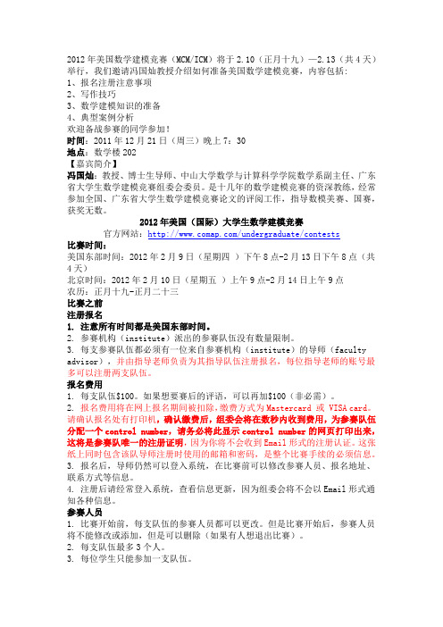
2012年美国数学建模竞赛(MCM/ICM)将于2.10(正月十九)—2.13(共4天)举行,我们邀请冯国灿教授介绍如何准备美国数学建模竞赛,内容包括:1、报名注册注意事项2、写作技巧3、数学建模知识的准备4、典型案例分析欢迎备战参赛的同学参加!时间:2011年12月21日(周三)晚上7:30地点:数学楼202【嘉宾简介】冯国灿:教授、博士生导师、中山大学数学与计算科学学院数学系副主任、广东省大学生数学建模竞赛组委会委员。
是十几年的数学建模竞赛的资深教练,经常参加全国、广东省大学生数学建模竞赛论文的评阅工作,指导数模美赛、国赛,获奖无数。
2012年美国(国际)大学生数学建模竞赛官方网站:/undergraduate/contests比赛时间:美国东部时间:2012年2月9日(星期四)下午8点-2月13日下午8点(共4天)北京时间:2012年2月10日(星期五)上午9点-2月14日上午9点农历:正月十九-正月二十三比赛之前注册报名1. 注意所有时间都是美国东部时间。
2. 参赛机构(institute)派出的参赛队伍没有数量限制。
3. 每支参赛队伍都必须有一位来自参赛机构(institute)的导师(faculty advisor),并由指导老师负责为其指导队伍注册报名,每位指导老师的账号最多可以注册两支队伍。
报名费用1. 每支队伍$100。
如果想要赛后的评语,可以再加$100(非必需)。
2.报名费用将在网上报名期间被扣除,缴费方式为Mastercard 或 VISA card。
请确认报名处有打印机,确认缴费后,组委会将在数秒内收到费用,为参赛队伍分配一个control number,请务必将此显示control number的网页打印出来,这将是参赛队唯一的注册证明,因为你将不会收到Email形式的注册认证。
这张纸上同时包含该队导师注册时使用的邮箱和密码,是整个比赛手续的必须信息。
3. 报名后,导师仍然可以登入系统,在比赛前可以修改参赛人员、报名地址、联系方式等信息。
2012年美国高中生数学建模竞赛特等奖论文

题目:How Much Gas Should I Buy This Week?题目来源:2012年第十五届美国高中生数学建模竞赛(HiMCM)B题获奖等级:特等奖,并授予INFORMS奖论文作者:深圳中学2014届毕业生李依琛、王喆沛、林桂兴、李卓尔指导老师:深圳中学张文涛AbstractGasoline is the bleed that surges incessantly within the muscular ground of city; gasoline is the feast that lures the appetite of drivers. “To fill or not fill?” That is the question flustering thousands of car owners. This paper will guide you to predict the gasoline prices of the coming week with the currently available data with respect to swift changes of oil prices. Do you hold any interest in what pattern of filling up the gas tank can lead to a lower cost in total?By applying the Time series analysis method, this paper infers the price in the imminent week. Furthermore, we innovatively utilize the average prices of the continuous two weeks to predict the next two week’s average price; similarly, employ the four-week-long average prices to forecast the average price of four weeks later. By adopting the data obtained from 2011and the comparison in different aspects, we can obtain the gas price prediction model :G t+1=0.0398+1.6002g t+−0.7842g t−1+0.1207g t−2+ 0.4147g t−0.5107g t−1+0.1703g t−2+ε .This predicted result of 2012 according to this model is fairly ideal. Based on the prediction model,We also establish the model for how to fill gasoline. With these models, we had calculated the lowest cost of filling up in 2012 when traveling 100 miles a week is 637.24 dollars with the help of MATLAB, while the lowest cost when traveling 200 miles a week is 1283.5 dollars. These two values are very close to the ideal value of cost on the basis of the historical figure, which are 635.24 dollars and 1253.5 dollars respectively. Also, we have come up with the scheme of gas fulfillment respectively. By analyzing the schemes of gas filling, we can discover that when you predict the future gasoline price going up, the best strategy is to fill the tank as soon as possible, in order to lower the gas fare. On the contrary, when the predicted price tends to decrease, it is wiser and more economic for people to postpone the filling, which encourages people to purchase a half tank of gasoline only if the tank is almost empty.For other different pattern for every week’s “mileage driven”, we calculate the changing point of strategies-changed is 133.33 miles.Eventually, we will apply the models -to the analysis of the New York City. The result of prediction is good enough to match the actual data approximately. However, the total gas cost of New York is a little higher than that of the average cost nationally, which might be related to the higher consumer price index in the city. Due to the limit of time, we are not able to investigate further the particular factors.Keywords: gasoline price Time series analysis forecast lowest cost MATLABAbstract ---------------------------------------------------------------------------------------1 Restatement --------------------------------------------------------------------------------------21. Assumption----------------------------------------------------------------------------------42. Definitions of Variables and Models-----------------------------------------------------4 2.1 Models for the prediction of gasoline price in the subsequent week------------4 2.2 The Model of oil price next two weeks and four weeks--------------------------5 2.3 Model for refuel decision-------------------------------------------------------------52.3.1 Decision Model for consumer who drives 100 miles per week-------------62.3.2 Decision Model for consumer who drives 200 miles per week-------------73. Train and Test Model by 2011 dataset---------------------------------------------------8 3.1 Determine the all the parameters in Equation ② from the 2011 dataset-------8 3.2 Test the Forecast Model of gasoline price by the dataset of gasoline price in2012-------------------------------------------------------------------------------------10 3.3 Calculating ε --------------------------------------------------------------------------12 3.4 Test Decision Models of buying gasoline by dataset of 2012-------------------143.4.1 100 miles per week---------------------------------------------------------------143.4.2 200 miles per week---------------------------------------------------------------143.4.3 Second Test for the Decision of buying gasoline-----------------------------154. The upper bound will change the Decision of buying gasoline---------------------155. An analysis of New York City-----------------------------------------------------------16 5.1 The main factor that will affect the gasoline price in New York City----------16 5.2 Test Models with New York data----------------------------------------------------185.3 The analysis of result------------------------------------------------------------------196. Summery& Advantage and disadvantage-----------------------------------------------197. Report----------------------------------------------------------------------------------------208. Appendix------------------------------------------------------------------------------------21 Appendix 1(main MATLAB programs) ------------------------------------------------21 Appendix 2(outcome and graph) --------------------------------------------------------34The world market is fluctuating swiftly now. As the most important limited energy, oil is much accounted of cars owners and dealer. We are required to make a gas-buying plan which relates to the price of gasoline, the volume of tank, the distance that consumer drives per week, the data from EIA and the influence of other events in order to help drivers to save money.We should use the data of 2011 to build up two models that discuss two situations: 100miles/week or 200miles/week and use the data of 2012 to test the models to prove the model is applicable. In the model, consumer only has three choices to purchase gas each week, including no gas, half a tank and full tank. At the end, we should not only build two models but also write a simple but educational report that can attract consumer to follow this model.1.Assumptiona)Assume the consumer always buy gasoline according to the rule of minimumcost.b)Ignore the difference of the gasoline weight.c)Ignore the oil wear on the way to gas stations.d)Assume the tank is empty at the beginning of the following models.e)Apply the past data of crude oil price to predict the future price ofgasoline.(The crude oil price can affect the gasoline price and we ignore thehysteresis effect on prices of crude oil towards prices of gasoline.)2.Definitions of Variables and Modelst stands for the sequence number of week in any time.(t stands for the current week. (t-1) stands for the last week. (t+1) stands for the next week.c t: Price of crude oil of the current week.g t: Price of gasoline of the t th week.P t: The volume of oil of the t th week.G t+1: Predicted price of gasoline of the (t+1)th week.α,β: The coefficient of the g t and c t in the model.d: The variable of decision of buying gasoline.(d=1/2 stands for buying a half tank gasoline)2.1 Model for the prediction of gasoline price in the subsequent weekWhether to buy half a tank oil or full tank oil depends on the short-term forecast about the gasoline prices. Time series analysis is a frequently-used method to expect the gasoline price trend. It can be expressed as:G t+1=α1g t+α2g t−1+α3g t−2+α4g t−3+…αn+1g t−n+ε ----Equation ①ε is a parameter that reflects the influence towards the trend of gasoline price in relation to several aspects such as weather data, economic data, world events and so on.Due to the prices of crude oil can influence the future prices of gasoline; we will adopt the past prices of crude oil into the model for gasoline price forecast.G t+1=(α1g t+α2g t−1+α3g t−2+α4g t−3+⋯αn+1g t−n)+(β1g t+β2g t−1+β3g t−2+β4g t−3+⋯βn+1g t−n)+ε----Equation ②We will use the 2011 data set to calculate the all coefficients and the best delay periods n.2.2 The Model of oil price next two weeks and four weeksWe mainly depend on the prediction of change of gasoline price in order to make decision that the consumer should buy half a tank or full tank gas. When consumer drives 100miles/week, he can drive whether 400miles most if he buys full tank gas or 200miles most if he buys half a tank gas. When consumer drives 200miles/week, full tank gas can be used two weeks most or half a tank can be used one week most. Thus, we should consider the gasoline price trend in four weeks in future.Equation ②can also be rewritten asG t+1=(α1g t+β1g t)+(α2g t−1+β2g t−1)+(α3g t−2+β3g t−2)+⋯+(αn+1g t−n+βn+1g t−n)+ε ----Equation ③If we define y t=α1g t+β1g t,y t−1=α2g t−1+β2g t−1, y t−2=α3g t−2+β3g t−2……, and so on.Equation ③can change toG t+1=y t+y t−1+y t−2+⋯+y t−n+ε ----Equation ④We use y(t−1,t)denote the average price from week (t-1) to week (t), which is.y(t−1,t)=y t−1+y t2Accordingly, the average price from week (t-3) to week (t) isy(t−3,t)=y t−3+y t−2+y t−1+y t.4Apply Time series analysis, we can get the average price from week (t+1) to week (t+2) by Equation ④,G(t+1,t+2)=y(t−1,t)+y(t−3,t−2)+y(t−5,t−4), ----Equation ⑤As well, the average price from week (t+1) to week (t+4) isG(t+1,t+4)=y(t−3,t)+y(t−7,t−4)+y(t−11,t−8). ----Equation ⑥2.3 Model for refuel decisionBy comparing the present gasoline price with the future price, we can decide whether to fill half or full tank.The process for decision can be shown through the following flow chart.Chart 1For the consumer, the best decision is to get gasoline with the lowest prices. Because a tank of gasoline can run 2 or 4 week, so we should choose a time point that the price is lowest by comparison of the gas prices at present, 2 weeks and 4 weeks later separately. The refuel decision also depends on how many free spaces in the tank because we can only choose half or full tank each time. If the free spaces are less than 1/2, we can refuel nothing even if we think the price is the lowest at that time.2.3.1 Decision Model for consumer who drives 100 miles per week.We assume the oil tank is empty at the beginning time(t=0). There are four cases for a consumer to choose a best refuel time when the tank is empty.i.g t>G t+4and g t>G t+2, which means the present gasoline price is higherthan that either two weeks or four weeks later. It is economic to fill halftank under such condition. ii. g t <Gt +4 and g t <G t +2, which means the present gasoline price is lower than that either two weeks or four weeks later. It is economic to fill fulltank under such condition. iii. Gt +4>g t >G t +2, which means the present gasoline price is higher than that two weeks later but lower than that four weeks later. It is economic to fillhalf tank under such condition. iv. Gt +4<g t <G t +2, which means the present gasoline price is higher than that four weeks later but lower than that two weeks later. It is economic to fillfull tank under such condition.If other time, we should consider both the gasoline price and the oil volume in the tank to pick up a best refuel time. In summary, the decision model for running 100 miles a week ist 2t 4t 2t 4t 2t 4t 2t 4t 11111411111ˆˆ(1)1((1)&max(,))24442011111ˆˆˆˆ1/2((1)&G G G (&))(0(1G G )&)4424411ˆˆˆ(1)0&(G 4G G (G &)t i t i t t t t i t i t t t t t t i t t d t or d t g d d t g or d t g d t g or ++++----+++-++<--<<--<>⎧⎪=<--<<<--<<<⎨⎪⎩--=><∑∑∑∑∑t 2G ˆ)t g +<----Equation ⑦d i is the decision variable, d i =1 means we fill full tank, d i =1/2 means we fill half tank. 11(1)4t i tdt ---∑represents the residual gasoline volume in the tank. The method of prices comparison was analyzed in the beginning part of 2.3.1.2.3.2 Decision Model for consumer who drives 200 miles per week.Because even full tank can run only two weeks, the consumer must refuel during every two weeks. There are two cases to decide whether to buy half or full tank when the tank is empty. This situation is much simpler than that of 100 miles a week. The process for decision can also be shown through the following flow chart.Chart 2The two cases for deciding buy half or full tank are: i. g t >Gt +1, which means the present gasoline price is higher than the next week. We will buy half tank because we can buy the cheaper gasoline inthe next week. ii. g t <Gt +1, which means the present gasoline price is lower than the next week. To buy full tank is economic under such situation.But we should consider both gasoline prices and free tank volume to decide our refueling plan. The Model is111t 11t 111(1)1220111ˆ1/20(1)((1)0&)22411ˆ(1&G )0G 2t i t t i t i t t t t t i t t d t d d t or d t g d t g ----++<--<⎧⎪=<--<--=>⎨⎪⎩--=<∑∑∑∑ ----Equation ⑧3. Train and Test Model by the 2011 datasetChart 33.1 Determine all the parameters in Equation ② from the 2011 dataset.Using the weekly gas data from the website and the weekly crude price data from , we can determine the best delay periods n and calculate all the parameters in Equation ②. For there are two crude oil price dataset (Weekly Cushing OK WTI Spot Price FOB and Weekly Europe Brent SpotPrice FOB), we use the average value as the crude oil price without loss of generality. We tried n =3, 4 and 5 respectively with 2011 dataset and received comparison graph of predicted value and actual value, including corresponding coefficient.(A ) n =3(the hysteretic period is 3)Graph 1 The fitted price and real price of gasoline in 2011(n=3)We find that the nearby effect coefficient of the price of crude oil and gasoline. This result is same as our anticipation.(B)n=4(the hysteretic period is 4)Graph 2 The fitted price and real price of gasoline in 2011(n=4)(C) n=5(the hysteretic period is 5)Graph 3 The fitted price and real price of gasoline in 2011(n=5)Via comparing the three figures above, we can easily found that the predictive validity of n=3(the hysteretic period is 3) is slightly better than that of n=4(the hysteretic period is 4) and n=5(the hysteretic period is 5) so we choose the model of n=3 to be the prediction model of gasoline price.G t+1=0.0398+1.6002g t+−0.7842g t−1+0.1207g t−2+ 0.4147g t−0.5107g t−1+0.1703g t−2+ε----Equation ⑨3.2 Test the Forecast Model of gasoline price by the dataset of gasoline price in 2012Next, we apply models in terms of different hysteretic periods(n=3,4,5 respectively), which are shown in Equation ②,to forecast the gasoline price which can be acquired currently in 2012 and get the graph of the forecast price and real price of gasoline:Graph 4 The real price and forecast price in 2012(n=3)Graph 5 The real price and forecast price in 2012(n=4)Graph 6 The real price and forecast price in 2012(n=5)Conserving the error of observation, predictive validity is best when n is 3, but the differences are not obvious when n=4 and n=5. However, a serious problem should be drawn to concerns: consumers determines how to fill the tank by using the trend of oil price. If the trend prediction is wrong (like predicting oil price will rise when it actually falls), consumers will lose. We use MATLAB software to calculate the amount of error time when we use the model of Equation ⑨to predict the price of gasoline in 2012. The graph below shows the result.It’s not difficult to find the prediction effect is the best when n is 3. Therefore, we determined to use Equation ⑨as the prediction model of oil price in 2012.G t+1=0.0398+1.6002g t+−0.7842g t−1+0.1207g t−2+ 0.4147g t−0.5107g t−1+0.1703g t−2+ε3.3 Calculating εSince political occurences, economic events and climatic changes can affect gasoline price, it is undeniable that a ε exists between predicted prices and real prices. We can use Equation ②to predict gasoline prices in 2011 and then compare them with real data. Through the difference between predicted data and real data, we can estimate the value of ε .The estimating process can be shown through the following flow chartChart 4We divide the international events into three types: extra serious event, major event and ordinary event according to the criteria of influence on gas prices. Then we evaluate the value: extra serious event is 3a, major event is 2a, and ordinary event is a. With inference to the comparison of the forecast price and real price in 2011, we find that large deviation of data exists at three time points: May 16,2011, Aug 08,2011 andOct 10,2011. After searching, we find that some important international events happened nearly at the three time points. We believe that these events which occurred by chance affect the international prices of gasoline so the predicted prices deviate from the actual prices. The table of events and the calculation of the value of a areTherefore, by generalizing several sets of particular data and events, we can estimate the value of a:a=26.84 ----Equation ⑩The calculating process is shown as the following graph.Since now we have obtained the approximate value of a, we can evaluate the future prices according to currently known gasoline prices and crude oil prices. To improve our model, we can look for factors resulting in some major turning point in the graph of gasoline prices. On the ground that the most influential factors on prices in 2012 are respectively graded, the difference between fact and prediction can be calculated.3.4 Test Decision Models of buying gasoline by the dataset of 2012First, we use Equation ⑨to calculate the gasoline price of next week and use Equation ⑤and Equation ⑥to calculate the gasoline price trend of next two to four weeks. On the basis above, we calculate the total cost, and thus receive schemes of buying gasoline of 100miles per week according to Equation ⑦and Equation ⑧. Using the same method, we can easily obtain the pattern when driving 200 miles per week. The result is presented below.We collect the important events which will affect the gasoline price in 2012 as well. Therefore, we calculate and adjust the predicted price of gasoline by Equation ⑩. We calculate the scheme of buying gasoline again. The result is below:3.4.1 100 miles per weekT2012 = 637.2400 (If the consumer drives 100 miles per week, the total cost inTable 53.4.2 200 miles per weekT2012 = 1283.5 (If the consumer drives 200 miles per week, the total cost in 2012 is 1283.5 USD). The scheme calculated by software is below:Table 6According to the result of calculating the buying-gasoline scheme from the model, we can know: when the gasoline price goes up, we should fill up the tank first and fill up again immediately after using half of gasoline. It is economical to always keep the tank full and also to fill the tank in advance in order to spend least on gasoline fee. However, when gasoline price goes down, we have to use up gasoline first and then fill up the tank. In another words, we need to delay the time of filling the tank in order to pay for the lowest price. In retrospect to our model, it is very easy to discover that the situation is consistent with life experience. However, there is a difference. The result is based on the calculation from the model, while experience is just a kind of intuition.3.4.3 Second Test for the Decision of buying gasolineSince the data in 2012 is historical data now, we use artificial calculation to get the optimal value of buying gasoline. The minimum fee of driving 100 miles per week is 635.7440 USD. The result of calculating the model is 637.44 USD. The minimum fee of driving 200 miles per week is 1253.5 USD. The result of calculating the model is 1283.5 USD. The values we calculate is close to the result of the model we build. It means our model prediction effect is good. (we mention the decision people made every week and the gas price in the future is unknown. We can only predict. It’s normal to have deviation. The buying-gasoline fee which is based on predicted calculation must be higher than the minimum buying-gasoline fee which is calculated when all the gas price data are known.)We use MATLAB again to calculate the total buying-gasoline fee when n=4 and n=5. When n=4,the total fee of driving 100 miles per week is 639.4560 USD and the total fee of driving 200 miles per week is 1285 USD. When n=5, the total fee of driving 100 miles per week is 639.5840 USD and the total fee of driving 200 miles per week is 1285.9 USD. The total fee are all higher the fee when n=3. It means it is best for us to take the average prediction model of 3 phases.4. The upper bound will change the Decision of buying gasoline.Assume the consumer has a mileage driven of x1miles per week. Then, we can use 200to indicate the period of consumption, for half of a tank can supply 200-mile x1driving. Here are two situations:<1.5①200x1>1.5②200x1In situation①, the consumer is more likely to apply the decision of 200-mile consumer’s; otherwise, it is wiser to adopt the decision of 100-mile consumer’s. Therefore, x1is a critical value that changes the decision if200=1.5x1x1=133.3.Thus, the mileage driven of 133.3 miles per week changes the buying decision.Then, we consider the full-tank buyers likewise. The 100-mile consumer buys half a tank once in four weeks; the 200-mile consumer buys half a tank once in two weeks. The midpoint of buying period is 3 weeks.Assume the consumer has a mileage driven of x2miles per week. Then, we can to illustrate the buying period, since a full tank contains 400 gallons. There use 400x2are still two situations:<3③400x2>3④400x2In situation③, the consumer needs the decision of 200-mile consumer’s to prevent the gasoline from running out; in the latter situation, it is wiser to tend to the decision of 100-mile consumer’s. Therefore, x2is a critical value that changes the decision if400=3x2x2=133.3We can find that x2=x1=133.3.To wrap up, there exists an upper bound on “mileage driven”, that 133.3 miles per week is the value to switch the decision for buying weekly gasoline. The following picture simplifies the process.Chart 45. An analysis of New Y ork City5.1 The main factors that will affect the gasoline price in New York CityBased on the models above, we decide to estimate the price of gasoline according to the data collected and real circumstances in several cities. Specifically, we choose New York City as a representative one.New York City stands in the North East in the United States, with the largest population throughout the country as 8.2 million. The total area of New York City is around 1300 km2, with the land area as 785.6 km2(303.3 mi2). One of the largest trading centers in the world, New York City has a high level of resident’s consumption. As a result, the level of the price of gasoline in New York City is higher than the average regular oil price of the United States. The price level of gasoline and its fluctuation are the main factors of buying decision.Another reasonable factor we expect is the distribution of gas stations. According to the latest report, there are approximately 1670 gas stations in the city area (However, after the impact of hurricane Sandy, about 90 gas stations have been temporarily out of use because of the devastation of Sandy, and there is still around 1580 stations remaining). From the information above, we can calculate the density of gas stations thatD(gasoline station)= t e amount of gas stationstotal land area =1670 stations303.3 mi2=5.506 stations per mi2This is a respectively high value compared with several other cities the United States. It also indicates that the average distance between gas stations is relatively small. The fact that we can neglect the distance for the cars to get to the station highlights the role of the fluctuation of the price of gasoline in New York City.Also, there are approximately 1.8 million residents of New York City hold the driving license. Because the exact amount of cars in New York City is hard to determine, we choose to analyze the distribution of possible consumers. Thus, we can directly estimate the density of consumers in New York City in a similar way as that of gas stations:D(gasoline consumers)= t e amount of consumerstotal land area = 1.8 million consumers303.3 mi2=5817consumers per mi2Chart 5In addition, we expect that the fluctuation of the price of crude oil plays a critical role of the buying decision. The media in New York City is well developed, so it is convenient for citizens to look for the data of the instant price of crude oil, then to estimate the price of gasoline for the coming week if the result of our model conforms to the assumption. We will include all of these considerations in our modification of the model, which we will discuss in the next few steps.For the analysis of New York City, we apply two different models to estimate the price and help consumers make the decision.5.2 Test Models with New York dataAmong the cities in US, we pick up New York as an typical example. The gas price data is downloaded from the website () and is used in the model described in Section 2 and 3.The gas price curves between the observed data and prediction data are compared in next Figure.Figure 6The gas price between the observed data and predicted data of New York is very similar to Figure 3 in US case.Since there is little difference between the National case and New York case, the purchase strategy is same. Following the same procedure, we can compare the gas cost between the historical result and predicted result.For the case of 100 miles per week, the total cost of observed data from Feb to Oct of 2012 in New York is 636.26USD, while the total cost of predicted data in the same period is 638.78USD, which is very close. It proves that our prediction model is good. For the case of 200 miles per week, the total cost of observed data from Feb to Oct of 2012 in New York is 1271.2USD, while the total cost of predicted data in the same period is 1277.6USD, which is very close. It proves that our prediction model is good also.5.3 The analysis of resultBy comparing, though density of gas stations and density of consumers of New York is a little higher than other places but it can’t lower the total buying-gas fee. Inanother words, density of gas stations and density of consumers are not the actual factors of affecting buying-gas fee.On the other hand, we find the gas fee in New York is a bit higher than the average fee in US. We can only analyze preliminary it is because of the higher goods price in New York. We need to add price factor into prediction model. We can’t improve deeper because of the limited time. The average CPI table of New York City and USA is below:Datas Statistics website(/xg_shells/ro2xg01.htm)6. Summery& Advantage and disadvantageTo reach the solution, we make graphs of crude oil and gasoline respectively and find the similarity between them. Since the conditions are limited that consumers can only drive 100miles per week or 200miles per week, we separate the problem into two parts according to the limitation. we use Time series analysis Method to predict the gasoline price of a future period by the data of several periods in the past. Then we take the influence of international events, economic events and weather changes and so on into consideration by adding a parameter. We give each factor a weight consequently and find the rules of the solution of 100miles per week and 200miles per week. Then we discuss the upper bound and clarify the definition of upper bound to solve the problem.According to comparison from many different aspects, we confirm that the model expressed byEquation ⑨is the best. On the basis of historical data and the decision model of buying gasoline(Equation ⑦and Equation ⑧), we calculate that the actual least cost of buying gasoline is 635.7440 USD if the consumer drives 100 miles per week (the result of our model is 637.24 USD) and the actual least cost of buying gasoline is 1253.5 USD(the result of our model is 1283.5 USD) if the consumer drives 100 miles per week. The result we predicted is similar to the actual result so the predictive validity of our model is finer.Disadvantages:1.The events which we predicted are difficult to quantize accurately. The turningpoint is difficult for us to predict accurately as well.2.We only choose two kinds of train of thought to develop models so we cannotevaluate other methods that we did not discuss in this paper. Other models which are built up by other train of thought are possible to be the optimal solution.。
MCM(MCM Mathematical Contest i

奖项
美国大学生数学建模竞赛共设置四个奖项,分别为 Outstanding Winner, Finalist, Meritorious Winner, Honorable Mentions, Successfully Participation。 在国内,约定俗成地将这四个奖项分别对应为特等奖、特等候选奖、一等奖、二等奖、成功参赛。
MCM(MCM Mathematical Contest i
MCM-Mathematical Contest in Modeling
01 简介
03 奖项
目录
02 历史背景 04 其他
《MCM》是MCM-Mathematical ContCM/ICM),是一项国际级的竞赛项目,为现今各类数学建模竞赛之鼻祖。
感谢观看
竞赛以三人(本科生)为一组,在四天时间内,就指定的问题完成从建立模型、求解、验证到论文撰写的全 部工作。竞赛每年都吸引大量著名高校参赛。2008年 MCM/ICM有超过 2000个队伍参加,遍及五大洲。MCM/ICM 已经成为最著名的国际大学生竞赛之一。
历史背景
1985年,在美国科学基金会的资助下,创办了一个名为“数学建模竞赛”(Mathematical Competition in Modeling后改名Mathematical Contest in Modeling,简称MCM)一年一度的大学水平的竞赛,MCM的宗旨是鼓 励大学师生对范围并不固定的各种实际问题予以阐明、分析并提出解法,通过这样一种结构鼓励师生积极参与并 强调实现完整的模型构造的过程。它是一种彻底公开的竞赛,每年只有若干个来自不受限制的任何领域的实际问 题,学生以三人组成一队的形式参赛,在三天(72小时)(近年改为四天,即96小时)内任选一题,完成该实际 问题的数学建模的全过程,并就问题的重述、简化和假设及其合理性的论述、数学模型的建立和求解(及软件)、 检验和改进、模型的优缺点及其可能的应用范围的自我评述等内容写出论文。由专家组成的评阅组进行评阅,评 出优秀论文,并给予某种奖励,它只有唯一的禁律,就是在竞赛期间不得与队外任何人(包括指导教师)讨论赛 题,但可以利用任何图书资料、互联网上的资料、任何类型的计算机和软件等,为充分发挥参赛学生的创造性提 供了广阔的空间。第一届MCM时,就有美国70所大学90个队参加,到1992年已经有美国及其它一些国家的189所大 学292个队参加,在某种意义下,已经成为一种国际性的竞赛,影响极其广泛。
美国大学生数学建模竞赛的命题与评阅指导课件

2. MCM/ICM 题目的不同之处
• ICM问题通常是全球关注的问题,不依赖于文化背景 • 这就更有利于中国学生。因为某些MCM问题有时
偏重文化与传统的背景,如MCM 2006B,机场轮椅 问题,MCM2021A,交通灯设计,Stop sign(路口暂时 停的标记牌),yield sign〔并道时必需看来车方向〕 在中国没有此类警示牌,MCM2021A, Ultimate Brownie Pan 等,很多中国学生无此概念。 • 参赛的学生根据自己的特长,选择不同类型的题目。
SOL GARFUNKEL, EXECUTIVE DIRECTOR, COMAP
“I hope that you will to work on the exciting and important problems you see here, and that you will join the MCM/ICM contest and rewarding work of increasing the awareness of the importance of Mathematical Modeling.〞
初评过程---论文分类
初评〔第一阶段triage judging〕,也称为鉴别评审阶段。 每篇论文在此阶段中按质量分为以下三类: 第一类是可以进入下一阶段评审的论文; 第二类是满足竞赛要求,但却缺乏以进入下一阶段评
审的论文,这类论文为合格论文; 第三类是不符合竞赛要求的论文,这类论文为不合格
论文。
31
Tianjin University
• Mathematical Modeling for the MCM/ICM Contest , Volume 2
• MCM/ICM评委 • 内容简介 • 1-4章:2021年4个竞赛题的分析、点评与解答 • 第5章:对数学建模研究当前热点问题的拓展 • 实用性强,可供参加美赛的读者参考使用
2012年 AMC8 美国数学竞赛试题+答案(英文版)
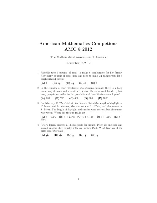
12. What is the units digit of 132012? (A) 1 (B) 3 (C) 5 (D) 7
(E) 9
13. Jamar bought some pencils costing more than a penny each at the school bookstore and paid $1.43. Sharona bought some of the same pencils and paid $1.87. How many more pencils did Sharona buy than Jamar?
(A) 5 : 10pm (B) 5 : 21pm (C) 5 : 41pm (D) 5 : 57pm (E) 6 : 03pm
4. Peter’s family ordered a 12-slice pizza for dinner. Peter ate one slice and shared another slice equally with his brother Paul. What fraction of the pizza did Peter eat?
(A) 3 (B) 4 (C) 5 (D) 6 (E) 7
18. What is the smallest positive integer that is neither prime nor square and that has no prime factor less than 50?
(A) 3127 (B) 3133 (C) 3137 (D) 3139 (E) 3149
22. Let R be a set of nine distinct integers. Six of the elements are 2, 3, 4, 6, 9, and 14. What is the number of possible values of the median of R ?
- 1、下载文档前请自行甄别文档内容的完整性,平台不提供额外的编辑、内容补充、找答案等附加服务。
- 2、"仅部分预览"的文档,不可在线预览部分如存在完整性等问题,可反馈申请退款(可完整预览的文档不适用该条件!)。
- 3、如文档侵犯您的权益,请联系客服反馈,我们会尽快为您处理(人工客服工作时间:9:00-18:30)。
破案模型您的组织,ICM正在调查一个作案阴谋。
调查者非常有信心,因为他们知道阴谋集团的几名成员,但他们希望在进行逮捕之前能找出其他成员和领导人。
主谋者和所有可能涉嫌同谋的人都以复杂的关系为同一家公司在一个大办公室工作。
这家公司一直快速增长,并在开发和销售适用于银行和信用卡公司的计算机软件方面打出了自己的名气。
ICM最近从一个82个工人的小集体那儿得知了一个消息,他们认为这个消息能将帮助他们在公司里找到目前身份尚不明确的同谋者和未知的领导人的最有可能的人选。
由于信息流通涉及到所有的在该公司工作的工人,所以很可能在这次信息流通中有一些(或许很多)已经确定的传播者实际并不涉及阴谋。
事实上,他们确定他们知道一些并不参与阴谋的人。
建模工作的目标是确定在这个复杂的办公室里谁是最有可能的同谋。
一个优先级列表是最理想的,因为ICM可以根据这个来调查,**,和/或询问最有可能的候选人。
一个划分非同谋者与同谋者的分割线也将是有益的,因为可以对每个组里的人进行清楚的分类。
如果能提名阴谋的领导人,那对于检察官办公室也是非常有帮助的。
在把当前情况下的数据给你的犯罪建模团队之前,你的上司给你以下情形(称为调查EZ),那是她几年前在另一座城市工作时的案例。
她对她在简单案件的工作非常自豪,她说,这是一个非常小的,简单的例子,但它可以帮助你了解自己的任务。
她的数据如下:她认为是同谋的十人分别为Anne#, Bob, Carol, Dave*, Ellen, Fred, George*, Harry, Inez, and Jaye#.(*表示之前已知的同谋,#表示事先已知的非同谋者)她对她的案件的28个消息记录按照她的分析依据主题进行了编号。
Anne to Bob:你今天为什么迟到了?(1)Bob to Carol:这该死的Anne总是看着我。
我并没有迟到。
(1)Carol to Dave: Anne 和 Bob又再为Bob的迟到吵架了。
(1)Dave to Ellen:我今天早上要见你。
你什么时候能来?把预算文件顺便带过来。
(2)Dave to Fred:我今天随时随地都可以去见你。
让我知道什么时候比较好。
我需要带预算文件吗?(2)Dave to George:我待会见你---有很多需要谈的。
我希望其他人都准备好。
获得这项权利?很重要。
(3)Harry to George:你似乎很紧张。
怎么回事?不用担心,我们的预算会好的。
(2)(4)Inez to George:我今天真的很累。
你呢,还好吗?(5)Jaye to Inez:也不怎么样今天(?)。
今天一起去吃午饭怎么样?(5)Inez to Jaye:幸好一切都很平静。
我已经精疲力竭,不能做午饭了今天。
抱歉!(5)George to Dave:现在来见我!(3)Jaye to Anne:你去吃午饭吗今天?(5)Dave to George:我没法去,现在正要去见Fred。
(3)George to Dave:见完他后到我这来。
(3)Anne to Carol:谁来监督一下Bob?他整天游手好闲的。
(1)Carol to Anne:别管他。
他和George and Dave合作得很好。
(1)George to Dave:这个很重要。
该死的Fred。
Ellen怎么样了?(3)Ellen to George:你和Dave谈过了吗?(3)George to Ellen:还没。
你呢?(3)Bob to Anne:我没有迟到。
而且你知道我午饭时间都在工作呢。
(1)Bob to Dave:告诉他们我没有迟到。
你了解我的。
(1)Ellen to Carol:联系Anne安排下个星期的预算会议日程,还有,帮我让George冷静点。
(2)Harry to Dave:你有没有注意到George今天看上去又很紧张/有压力?(4)Dave to George:该死的Harry觉得你很紧张。
别让他担心,免得他四处打探。
(4)George to Harry:我只是工作得太晚,家里又有点问题。
不用担心,我很好。
(4)Ellen to Harry:我忘了今天的会议了,怎么办?Fred会在那的,而且他比我更了解预算。
(2)Harry to Fred:我觉得明年的预算会让一些人很有压力的。
或许你今天该花点时间让大家安心。
(2)(4)Fred to Harry:我觉得我们的预算很正常,我没觉得会有人感到有压力。
(2)通信记录结束。
你的上司指出,她只分配和编号了5个不同的消息主题:1)Bob的迟到,2)预算,3)重要的未知的问题,可能是阴谋,4)乔治的压力,5)午餐和其他社会问题。
正如看到的消息编码那样,一些消息根据内容有两个主题。
你的上司按照通信联系和消息类型构造的通信网络分析案件。
下图是一个消息网络模型,网络图上注明了消息类型的代码。
您的上司说,除了已知的同谋George and Dave之外,根据她的分析Ellen and Carol也被认为是同谋。
而且不久后,Bob招认出他确实参与其中,从而希望得到减刑。
而对Carol的控告后来被放弃了。
你的上司至今仍然相当肯定Inez也参与了,但却从未对她立案。
你的上司建议您的团队,确定有罪的当事人,使像Inez的人不漏网,像Carol的人不被诬陷,从而增加ICM的信用,使像Bob的人不再有获得减刑的机会。
现在的案件:你的上司已经把目前的情况下构造成网络状的数据库,它具有和上面相同的结构,只是范围较大。
调查者有一些线索表明,一个阴谋正在挪用公司的资金和使用网上诈骗盗窃在该公司做业务的顾客的信用卡资金。
她给你看的简单案件的小例子,只有10个人(节点),27条边(消息),5个主题,1个可疑/阴谋主题,2个确定的罪犯,2个已知的清白者。
而到目前为止,这个新的案件却已经有83个节点,400条边(有些不止涉及1个主题),超过21000个单词的消息记录,15个主题(其中3个已被视为是可疑的),7个已知的罪犯,和8个已知的清白者。
这些数据在所附的电子表格文件:names.xls,Topics.xls,Messages.xls中给出。
names.xls包含办公室的关键节点对应的员工的名字。
topics.xls包含15个主题的代号及简短说明。
由于安全和隐私问题,你的团队不会有所有的直接消息记录。
messages.xls提供传输消息的节点对,和该消息的主题(可能不止一个主题,最多3个主题)。
为了使信息的沟通更加直观可视,图2提供了员工和消息链接的网络模型。
在这种情况下,不再像图1那样显示消息的主题。
而是在文件Messages.xls里给出主题的数目,并在Topics.xls中给以描述。
要求:要求1:到目前为止,已知Jean, Alex, Elsie, Paul, Ulf, Yao, and Harvey是罪犯,Darlene, Tran, Jia, Ellin, Gard, Chris, Paige, and Este不是罪犯。
可以的消息主题是7,11和13。
关于主题更多的信息在Topics.xls里。
建立模型和算法,把83个节点按照他是阴谋者的可能性大小排序,并解释你的模型和指标。
Jerome, Delores, and Gretchen是该公司的高级经理。
如果他们三个人中任何一个涉及阴谋这将是非常有益的。
要求2:优先列表将有神秘变化,如果有新的信息告知我们说主题1也与阴谋有关,而且克里斯是一个阴谋?(即多了两个线索)要求3:一个强大的与这个消息流通网络类似的获取和理解文本信息的技术被称为语义网络分析(semantic network analysis);作为人工智能和计算语言学的方法,它提供了一个结构,并可进行有关知识或语言的推理过程。
另一个有关自然语言处理的计算语言学是文本分析text analysis。
针对我们的破案的情况,解释:如果你能获得原始消息,那么对信息流量的上下文和内容进行语义和文字分析对于帮助你们的团队开发出更好的模型和办公室人员的分类有多大的帮助和加强作用?你有没有使用这些基于文件Topics.xls中的主题描述的功能来提高您的模型?要求4:你的完整报告将最终提交给检察官办公室,所以一定要详细、明确地说明您的假设和方法,但不能超过20页。
您可以包括你的程序作为单独的文件中的附件使你的论文不超过页面限制,但包括这些程序不是必须的。
你的上司希望ICM是世界最好的解决白领、高科技的阴谋罪的机构,并希望您的方法有助于解决重要的世界各地的案件,特别是那些消息流量非常大的数据库(可能有数万的信息和数百万的单词)。
她特别要求你在论文中讨论:更深入的网络,语义,消息的文本分析内容是如何帮助你的模型和建议的。
作为给她的报告的一部分,请解释你用到的网络模型技术,以及为什么使用和它们可以怎么被用于任何类型的网络数据库从而来确定,优先级排序,和对相似结点分类的技术的网络模型,而不仅仅是犯罪阴谋和消息数据。
比如,给你各种图像或化学数据,其中表明了感染概率和已经确定了的一些受感染的结点,你的方法能用来在生物网络中找到感染或患病的细胞吗?。