Application_of_COMSOL_in_Image_ Processing

1< p < 2
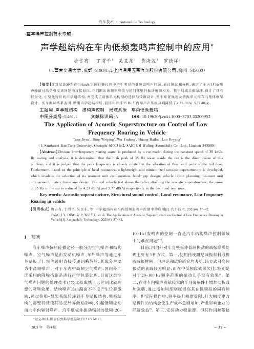
3、Implementation of PDE models in the COMOSL Multiphysics
Add Physics
Import the initial image
Draw the image domain Set the coefficient、 boundary and initial values Mesh
Add noise
Fig 2 original interferogram
Fig 3 noise interferogram
Fig 4 linear diffusion result
Fig 5 PM model result
Fig 6 TV model result
Coupled PDE model in image processing
1、Introduction
• Subject background
Fig 1 Experimental interferogram
• The interferogram from the Interferometric Synthetic Aperture Sonar (InSAS) has much noise because of the sonar shadow、water environment、under Sampling etc. The noise will make the following phase unwrapping become very difficult. So it is important for InSAS to denoise the interferogram effectively.
• 1、Introduction
• 2、PDE models in image processing • 3、Implementation of PDE models in the COMSOL Multiphysics • 4、Experimental results and data analysis • 5、Conclusion and outlook
2、PDE models in image processing
• 2.1 The general form of PDE in image processing
⎧ ∂u 2 t , x + F x , u t , x , ∇ u t , x , ∇ 在 ( 0, T ) × Ω上， ( ) ( ) ( ) ( x x u ( t , x ) ) = 0, ⎪ ∂t ⎪ ⎪ ∂u 在 ( 0, T ) × Ω上， ⎨ ( t , x ) |∂Ω = 0, ⎪ ∂n ⎪u ( 0, x ) = u0 ( x ) , 在Ω内， ⎪ ⎩ • Where Ω ⊂ R2is the image domain, ∂Ω is the boundary Ω of of is the initial F ∂Ω u n , is unit normal vector 0 ( x) ,
2 ⎧ ∂u ⎪ ∂t = ∇ ⋅ c ∇u ∇u , ⎪ ⎪ ∂u ⎨ |∂Ω = 0, ⎪ ∂n ⎪u ( 0, x ) = u0 ( x ) , ⎪ ⎩
(( ) )
在 ( 0,T ) × Ω内, 在 ( 0,T ) × ∂Ω上, 在Ω内,
• It is a an anisotropy diffusion equation. Where c ∇u is a diffusion function depended on the image gradient. P-M model can denoise and preserve edges well by defining the diffusion function suitably.
the edge function defined as gk (s) = 1 1 + s 2 k 2 . • It is a coupled PDE model, which can preserve the image edges well when the image gradient ∇u changes a lot.
5、Conclusion and outlook
• Conclusion
• This paper introduces the basic ideas and theoretical frame of image processing based on PDE, presents the idea of the application of COMSOL Multiphysics in image processing. • The simulated and real lake experimental interferogram was denoised by the PDE models which are implemented in the COMSOL Multiphysics.The experimental results indicate that COMSOL Multiphysics is able to provide a new finite element simulation platform for image processing.
Ideas of this paper
• PDE is an important tool in image processing. COMSOL Multiphysics builds the models based on PDE，it is easy to define and solve the coupled problem of any physical field. • However, it has not the image processing module so far. So the idea is that COMSOL Multiphysics can be a new platform for image processing.
image. It can denoise the interferogram, however, it can not preserve the edges of image.
PDE models in image processing
• 2.3 Perona-Malik model in image processing
(
)
• Where λ is the lagrange multiplier depended on noise level. The model can overcome the staircase effect as long as we choose the proper p .
1 λ p 2 min J p ( u ) = ∫ ∇u dxdy + ∫ u − u0 dxdy, u pΩ 2Ω
• Coupled PDE model in image processing
∇u ⎧ ∂ u = α g ( ∇ v ) ∇ u div ( ) + α∇( g k ( ∇v )) ⋅∇u − β (u − I ) ∇u k ⎪ t ∇u ⎪ ⎪ ∇v ) − b (v − u ) ⎨∂ t v = a (t )div( ∇v ⎪ ⎪u ( x, y, 0) = u ( x, y ), v( x, y, 0) = u ( x, y ) 0 0 ⎪ ⎩ • Where I , u0 ( x, y ) are all the original noise image, g k ( s ) is
2s
5s
Fig 8 experimental interferogram
Fig 9 2s Coupled model filter result
Fig 10 5s Coupled model filter result
Table 1 Data analysis of the denoising results Interferogram data Lake experiment interferogram Solve time 0s 2s 5s Residues 1834 36 12
(
)
Experimental results and analysis
• The interferogram obtained by the InSAS lake experiment is denoised by Coupled PDE model which is built on the COMSOL Multiphysics, the experimental results and data analysis is
2011年中国区用户年会
Application of COMSOL in Image Processing
Speaker：Wang Maolin Supervisor：Yue Jun Qingdao Technological University October 18, 2011,Beijing
The outline of the report
(
2age processing
• 2.4 TV model in image processing p−2 ⎧ ∂u 2 t , x = ∇ ⋅ ∇ u ∇ u + λ u − u , t ≥ 0, x = x , x ∈ R , ( ) ( ) ( ) 0 1 2 ⎪ ∂t ⎪ ⎪ ∂u 在 ( 0,T ) × ∂Ω上, ⎨ ( t , x ) |∂Ω = 0, ⎪ ∂n ⎪u ( 0, x ) = u0 ( x )， 在Ω内， ⎪ ⎩ • It is obtained by minimize the following function