5.1-5.3 Mathematical induction
抽象代数——精选推荐

抽象代数⼀、课程⽬的与教学基本要求本课程是在学⽣已学习⼤学⼀年级“⼏何与代数”必修课的基础上,进⼀步学习群、环、域三个基本的抽象的代数结构。
要求学⽣牢固掌握关于这三种抽象的代数结构的基本事实、结果、例⼦。
对这三种代数结构在别的相关学科,如数论、物理学等的应⽤有⼀般了解。
⼆、课程内容第1章准备知识(Things Familiar and Less Familiar)10课时复习集合论、集合间映射及数学归纳法知识,通过学习集合间映射为继续学习群论打基础。
1、⼏个注记(A Few Preliminary Remarks)2、集论(Set Theory)3、映射(Mappings)4、A(S)(The Set of 1-1 Mappings of S onto Itself)5、整数(The Integers)6、数学归纳法(Mathematical Induction)7、复数(Complex Numbers)第2章群(Groups) 22课时建⽴关于群、⼦群、商群及直积的基本概念及基本性质;通过实例帮助建⽴抽象概念,掌握群同态定理及其应⽤;了解有限阿贝尔群的结构。
1、群的定义和例⼦(Definitions and Examples of Groups)2、⼀些简单注记(Some Simple Remarks)3、⼦群(Subgroups)4、拉格朗⽇定理(Lagrange’s Theorem)5、同态与正规⼦群(Homomorphisms and Normal Subgroups)6、商群(Factor Groups)7、同态定理(The Homomorphism Theorems)8、柯西定理(Cauchy’s Theorem)9、直积(Direct Products)10、有限阿贝尔群(Finite Abelian Groups) (选讲)11、共轭与西罗定理(Conjugacy and Sylow’s Theorem)(选讲)第3章对称群(The Symmetric Group) 8课时掌握对称群的结构定理,了解单群的概念及例⼦。
MathematicalInduction.ppt
CS 202 Epp, chapter 4 Aaron Bloomfield
1
How do you climb infinite stairs?
• Not a rhetorical question!
• First, you get to the base platform of the staircase
• Recall the inductive hypothesis:
k
2i 1 k 2
i 1
• Proof of inductive step:
k 1
2i 1 (k 1)2
i 1 k
2(k 1) 1 2i 1 k 2 2k 1 i 1 2k 1
• Three parts:
– Base case(s): show it is true for one element
• (get to the stair’s base platform)
– Inductive hypothesis: assume it is true for any given element
• Show that the sum of the first n odd
integers is n2
– Example: If n = 5, 1+3+5+7+9 = 25 = 52
– Formally, show:
n
n P(n) whereP(n) 2i 1 n2
i 1
• Base case: Show that P(1) is true
• Then, show that if it’s true for some value n, then it is true for n+1
数学归纳法

骨牌一个接一个倒下,就如同一个值到下一个值的过程。
1.证明当n = 1 时命题成立。
2.证明如果在n = m时命题成立,那么可以推导出在n = m+1 时命题也成立。
(m代表任意自然数)这种方法的原理在于:首先证明在某个起点值时命题成立,然后证明从一个值到下一个值的过程有效。
当这两点都已经证明,那么任意值都可以通过反复使用这个方法推导出来。
把这个方法想成多米诺效应也许更容易理解一些。
例如:你有一列很长的直立着的多米诺骨牌,如果你可以:1.证明第一张骨牌会倒。
2.证明只要任意一张骨牌倒了,那么与其相邻的下一张骨牌也会倒。
那么便可以下结论:所有的骨牌都会倒。
[编辑]例子假设我们要证明下面这个公式(命题):其中n为任意自然数。
这是用于计算前n个自然数的和的简单公式。
证明这个公式成立的步骤如下。
[编辑]证明[编辑]第一步第一步是验证这个公式在n = 1时成立。
我们有左边 = 1,而右边 = 1(1 + 1) / 2 = 1,所以这个公式在n = 1时成立。
第一步完成。
[编辑]第二步第二步我们需要证明如果假设n = m时公式成立,那么可以推导出n = m+1 时公式也成立。
证明步骤如下。
我们先假设n = m时公式成立。
即(等式 1)然后在等式等号两边分别加上m + 1 得到(等式 2)这就是n = m+1 时的等式。
我们现在需要根据等式 1 证明等式 2 成立。
通过因式分解合并,等式 2 的右手边也就是说这样便证明了从 P(m) 成立可以推导出 P(m+1) 也成立。
证明至此结束,结论:对于任意自然数n,P(n) 均成立。
[编辑]解释在这个证明中,归纳推理的过程如下:1.首先证明 P(1) 成立,即公式在n = 1 时成立。
2.然后证明从 P(m) 成立可以推导出 P(m+1) 也成立。
(这里实际应用的是演绎推理法)3.根据上两条从 P(1) 成立可以推导出 P(1+1),也就是 P(2) 成立。
4.继续推导,可以知道 P(3)成立。
数学符号公式缩写的英文发音

数学符号公式缩写的英文发音数学缩写列表this article is a listing of abbreviated names of mathematical functions, function-like operators and other mathematical terminology.这篇文章是一个数学函数,类似于函数的操作符和其他的数学术语的缩写名列表。
this list is limited to abbreviations of two or more letters. the capitalization of some of these abbreviations is not standardized – different authors use different capitalizations.this list is inplete; you can help by expanding it.这个列表受限于两个或更多字母的缩略语。
其中,一些缩略语字母大写并不是标准的 - 不同的使用不同的大写形式。
ac – axiom of choice.[1] 选择公理a.c. – absolutely continuous. 绝对连续的acrd – inverse chord function. 逆弦函数adj – adjugate of a matrix. 矩阵的伴随矩阵a.e. – almost everywhere. 殆遍,几乎处处ai – airy function. 艾里函数al – action limit. 处置界限alt – alternating group (alt(n) is also written as an.) 交错群a.m. – arithmetic mean. 算数平均数arccos – inverse cosine function. 反余弦函数arccosec – inverse cosecant function. (also written as arccsc.) 反余割函数arccot – inverse cotangent function. 反余切函数arccsc – inverse cosecant function. (also written as arccosec.) 反余割函数arcexc – inverse excosecant function. (also written as arcexcsc, arcexcosec.) 反外余割函数arcexcosec – inverse excosecant function. (also written as arcexcsc, arcexc.) 反外余割函数arcexcsc – inverse excosecant function. (also written as arcexcosec, arcexc.) 反外余割函数arcexs – inverse exsecant function. (also written as arcexsec.) 反外正割函数arcexsec – inverse exsecant function. (also written as arcexs.) 反外正割函数arcosech – inverse hyperbolic cosecant function. (also written as arcsch.) 反双曲余割函数arcosh – inverse hyperbolic cosine function. 反双曲余弦函数arcoth – inverse hyperbolic cotangent function. 反双曲余切函数arcsch – inverse hyperbolic cosecant function. (also written as arcosech.) 反双曲余割函数arcsec – inverse secant function. 反正割函数arcsin – inverse sine function. 反正弦函数arctan – inverse tangent function. 反正切函数arctan2 – inverse tangent function with two arguments. (also written as atan2.) 带有2个参数的反正切函数arg – argument of a plex number.[2] 复数的参数arg max – argument of the maximum. 最大值时的参数arg min – argument of the minimum. 最小值时的参数arsech – inverse hyperbolic secant function. 反双曲正割函数arsinh – inverse hyperbolic sine function. 反双曲正弦函数artanh – inverse hyperbolic tangent function. 反双曲正切函数a.s. – almost surely. 殆必,几乎必然atan2 – inverse tangent function with two arguments. (also written as arctan2.) 同 arctan2,带有两个参数的反正切函数a.p. – arithmetic progression. 等差数列aut – automorphism group. 自同构群bd – boundary. 边界(拓扑学)bi – airy function of the second kind. 第二类艾里函数bias – bias of an estimator 估计器偏置card – cardinality of a set.[3] (card(x) is also written #x, ♯x or |x|.) 集合的势cdf – cumulative distribution function. 累积分布函数c.f. – cumulative frequency. 累积频率char – characteristic of a ring. 环的特征chi – hyperbolic cosine integral function. 双曲余弦积分函数ci – cosine integral function. 余弦积分函数cis – cos + i sin function. 欧拉公式函数cl – conjugacy class. 共轭类cl – topological closure. 拓扑学闭包cod, codom – codomain. 到达域cok, coker – cokernel. 上核,余核cor – corollary. 推论,余定理corr – correlation. 相关cos – cosine function. 余弦函数割函数cosech – hyperbolic cosecant function. (also written as csch.) 双曲余割函数cosh – hyperbolic cosine function. 双曲余弦函数cosiv – coversine function. (also written as cover, covers, cvs.) 余矢函数cot – cotangent function. (also written as ctg.) 余切函数coth – hyperbolic cotangent function. 双曲余切函数cov – covariance of a pair of random variables. 协方差cover – coversine function. (also written as covers, cvs, cosiv.) 余矢函数covercos – covercosine function. (also written as cvc.) 正矢函数covers – coversine function. (also written as cover, cvs, cosiv.) 余矢函数crd – chord function. 弦(几何)函数csc – cosecant function. (also written as cosec.) 余割函数csch – hyperbolic cosecant function. (also written as cosech.) 双曲余割函数函数curl – curl of a vector field. (also written as rot.) 向量场的旋度cvc – covercosine function. (also written as covercos.) 余余矢函数cvs – coversine function. (also written as cover, covers, cosiv.) 正余矢函数def – define or definition. 定义deg – degree of a polynomial. (also written as ∂.)多项式的次数del – del, a differential operator. (also writtenas .) 微分运算符det – determinant of a matrix or linear transformation. 矩阵或线性变换的行列式dim – dimension of a vector space. 向量空间的维度div – divergence of a vector field. 向量场的散度dkl – decalitre 公斗。
数理逻辑 第三章 数学推理 数学归纳法

这样就证明了从P(n)得出P(n+1) 在第二个等式中我们使用了归纳假设P(n) 因为P(1)为真,而且对所有正整数n来说
P(n)→P(n+1)为真,所以,由数学归纳法原 理就证明了对所有正整数n来说P(n)为真
四、数学归纳法的例子
例:用数学归纳法证明:对所有正整数n 来说不等式n<2n
来说P(k)为真,要完成归纳步骤就必须证明 在这个假定下P(n+1)为真
五、数学归纳法的第二原理
例:证明:若n是大于1的整数,则n可以 写成素数之积
解:分两种情况考虑:当n+1是素数时和当 n+1是合数时。若n+1是素数,则P(n+1)为 真;若n+1是合数,则可以将其表示成两个 整数a和b之积,其中a、b满足 2≤a≤b≤n+1
3.2 数学归纳法 Mathematical Induction
一、引言
前n个正奇数之和的公式是什么? 对n=1,2,3,4,5来说,前n个正奇数之和为:
1=1,1+3=4,1+3+5=9, 1+3+5+7=16,1+3+5+7+9=25
猜测前n个正奇数之和是n2 假如这个猜测是正确的,我们就需要一
三、数学归纳法
用数学归纳法证明定理时
首先证明P(1)为真,然后知道P(2)为真,因 为P(1)蕴含P(2)
P(3)为真,因为P(2)蕴含P(3) 以这样的方式继续下去,就可以看出对任
意正整数k来说P(k)为真
数学归纳法的形象解释
三、数学归纳法
为什么数学归纳法是有效的?
《数据结构与算法分析》(C++第二版)【美】Clifford A.Shaffer著 课后习题答案 二
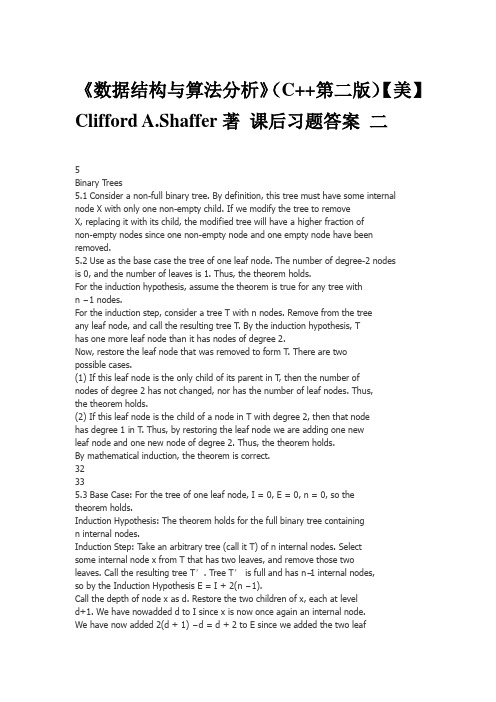
《数据结构与算法分析》(C++第二版)【美】Clifford A.Shaffer著课后习题答案二5Binary Trees5.1 Consider a non-full binary tree. By definition, this tree must have some internalnode X with only one non-empty child. If we modify the tree to removeX, replacing it with its child, the modified tree will have a higher fraction ofnon-empty nodes since one non-empty node and one empty node have been removed.5.2 Use as the base case the tree of one leaf node. The number of degree-2 nodesis 0, and the number of leaves is 1. Thus, the theorem holds.For the induction hypothesis, assume the theorem is true for any tree withn − 1 nodes.For the induction step, consider a tree T with n nodes. Remove from the treeany leaf node, and call the resulting tree T. By the induction hypothesis, Thas one more leaf node than it has nodes of degree 2.Now, restore the leaf node that was removed to form T. There are twopossible cases.(1) If this leaf node is the only child of its parent in T, then the number ofnodes of degree 2 has not changed, nor has the number of leaf nodes. Thus,the theorem holds.(2) If this leaf node is the child of a node in T with degree 2, then that nodehas degree 1 in T. Thus, by restoring the leaf node we are adding one newleaf node and one new node of degree 2. Thus, the theorem holds.By mathematical induction, the theorem is correct.32335.3 Base Case: For the tree of one leaf node, I = 0, E = 0, n = 0, so thetheorem holds.Induction Hypothesis: The theorem holds for the full binary tree containingn internal nodes.Induction Step: Take an arbitrary tree (call it T) of n internal nodes. Selectsome internal node x from T that has two leaves, and remove those twoleaves. Call the resulting tree T’. Tree T’ is full and has n−1 internal nodes,so by the Induction Hypothesis E = I + 2(n − 1).Call the depth of node x as d. Restore the two children of x, each at leveld+1. We have nowadded d to I since x is now once again an internal node.We have now added 2(d + 1) − d = d + 2 to E since we added the two leafnodes, but lost the contribution of x to E. Thus, if before the addition we had E = I + 2(n − 1) (by the induction hypothesis), then after the addition we have E + d = I + d + 2 + 2(n − 1) or E = I + 2n which is correct. Thus,by the principle of mathematical induction, the theorem is correct.5.4 (a) template <class Elem>void inorder(BinNode<Elem>* subroot) {if (subroot == NULL) return; // Empty, do nothingpreorder(subroot->left());visit(subroot); // Perform desired actionpreorder(subroot->right());}(b) template <class Elem>void postorder(BinNode<Elem>* subroot) {if (subroot == NULL) return; // Empty, do nothingpreorder(subroot->left());preorder(subroot->right());visit(subroot); // Perform desired action}5.5 The key is to search both subtrees, as necessary.template <class Key, class Elem, class KEComp>bool search(BinNode<Elem>* subroot, Key K);if (subroot == NULL) return false;if (subroot->value() == K) return true;if (search(subroot->right())) return true;return search(subroot->left());}34 Chap. 5 Binary Trees5.6 The key is to use a queue to store subtrees to be processed.template <class Elem>void level(BinNode<Elem>* subroot) {AQueue<BinNode<Elem>*> Q;Q.enqueue(subroot);while(!Q.isEmpty()) {BinNode<Elem>* temp;Q.dequeue(temp);if(temp != NULL) {Print(temp);Q.enqueue(temp->left());Q.enqueue(temp->right());}}}5.7 template <class Elem>int height(BinNode<Elem>* subroot) {if (subroot == NULL) return 0; // Empty subtreereturn 1 + max(height(subroot->left()),height(subroot->right()));}5.8 template <class Elem>int count(BinNode<Elem>* subroot) {if (subroot == NULL) return 0; // Empty subtreeif (subroot->isLeaf()) return 1; // A leafreturn 1 + count(subroot->left()) +count(subroot->right());}5.9 (a) Since every node stores 4 bytes of data and 12 bytes of pointers, the overhead fraction is 12/16 = 75%.(b) Since every node stores 16 bytes of data and 8 bytes of pointers, the overhead fraction is 8/24 ≈ 33%.(c) Leaf nodes store 8 bytes of data and 4 bytes of pointers; internal nodesstore 8 bytes of data and 12 bytes of pointers. Since the nodes havedifferent sizes, the total space needed for internal nodes is not the sameas for leaf nodes. Students must be careful to do the calculation correctly,taking the weighting into account. The correct formula looks asfollows, given that there are x internal nodes and x leaf nodes.4x + 12x12x + 20x= 16/32 = 50%.(d) Leaf nodes store 4 bytes of data; internal nodes store 4 bytes of pointers. The formula looks as follows, given that there are x internal nodes and35x leaf nodes:4x4x + 4x= 4/8 = 50%.5.10 If equal valued nodes were allowed to appear in either subtree, then during a search for all nodes of a given value, whenever we encounter a node of that value the search would be required to search in both directions.5.11 This tree is identical to the tree of Figure 5.20(a), except that a node with value 5 will be added as the right child of the node with value 2.5.12 This tree is identical to the tree of Figure 5.20(b), except that the value 24 replaces the value 7, and the leaf node that originally contained 24 is removed from the tree.5.13 template <class Key, class Elem, class KEComp>int smallcount(BinNode<Elem>* root, Key K);if (root == NULL) return 0;if (KEComp.gt(root->value(), K))return smallcount(root->leftchild(), K);elsereturn smallcount(root->leftchild(), K) +smallcount(root->rightchild(), K) + 1;5.14 template <class Key, class Elem, class KEComp>void printRange(BinNode<Elem>* root, int low,int high) {if (root == NULL) return;if (KEComp.lt(high, root->val()) // all to leftprintRange(root->left(), low, high);else if (KEComp.gt(low, root->val())) // all to rightprintRange(root->right(), low, high);else { // Must process both childrenprintRange(root->left(), low, high);PRINT(root->value());printRange(root->right(), low, high);}}5.15 The minimum number of elements is contained in the heap with a single node at depth h − 1, for a total of 2h−1 nodes.The maximum number of elements is contained in the heap that has completely filled up level h − 1, for a total of 2h − 1 nodes.5.16 The largest element could be at any leaf node.5.17 The corresponding array will be in the following order (equivalent to level order for the heap):12 9 10 5 4 1 8 7 3 236 Chap. 5 Binary Trees5.18 (a) The array will take on the following order:6 5 3 4 2 1The value 7 will be at the end of the array.(b) The array will take on the following order:7 4 6 3 2 1The value 5 will be at the end of the array.5.19 // Min-heap classtemplate <class Elem, class Comp> class minheap {private:Elem* Heap; // Pointer to the heap arrayint size; // Maximum size of the heapint n; // # of elements now in the heapvoid siftdown(int); // Put element in correct placepublic:minheap(Elem* h, int num, int max) // Constructor{ Heap = h; n = num; size = max; buildHeap(); }int heapsize() const // Return current size{ return n; }bool isLeaf(int pos) const // TRUE if pos a leaf{ return (pos >= n/2) && (pos < n); }int leftchild(int pos) const{ return 2*pos + 1; } // Return leftchild posint rightchild(int pos) const{ return 2*pos + 2; } // Return rightchild posint parent(int pos) const // Return parent position { return (pos-1)/2; }bool insert(const Elem&); // Insert value into heap bool removemin(Elem&); // Remove maximum value bool remove(int, Elem&); // Remove from given pos void buildHeap() // Heapify contents{ for (int i=n/2-1; i>=0; i--) siftdown(i); }};template <class Elem, class Comp>void minheap<Elem, Comp>::siftdown(int pos) { while (!isLeaf(pos)) { // Stop if pos is a leafint j = leftchild(pos); int rc = rightchild(pos);if ((rc < n) && Comp::gt(Heap[j], Heap[rc]))j = rc; // Set j to lesser child’s valueif (!Comp::gt(Heap[pos], Heap[j])) return; // Done37swap(Heap, pos, j);pos = j; // Move down}}template <class Elem, class Comp>bool minheap<Elem, Comp>::insert(const Elem& val) { if (n >= size) return false; // Heap is fullint curr = n++;Heap[curr] = val; // Start at end of heap// Now sift up until curr’s parent < currwhile ((curr!=0) &&(Comp::lt(Heap[curr], Heap[parent(curr)]))) {swap(Heap, curr, parent(curr));curr = parent(curr);}return true;}template <class Elem, class Comp>bool minheap<Elem, Comp>::removemin(Elem& it) { if (n == 0) return false; // Heap is emptyswap(Heap, 0, --n); // Swap max with last valueif (n != 0) siftdown(0); // Siftdown new root valit = Heap[n]; // Return deleted valuereturn true;}38 Chap. 5 Binary Trees// Remove value at specified positiontemplate <class Elem, class Comp>bool minheap<Elem, Comp>::remove(int pos, Elem& it) {if ((pos < 0) || (pos >= n)) return false; // Bad posswap(Heap, pos, --n); // Swap with last valuewhile ((pos != 0) &&(Comp::lt(Heap[pos], Heap[parent(pos)])))swap(Heap, pos, parent(pos)); // Push up if largesiftdown(pos); // Push down if small keyit = Heap[n];return true;}5.20 Note that this summation is similar to Equation 2.5. To solve the summation requires the shifting technique from Chapter 14, so this problem may be too advanced for many students at this time. Note that 2f(n) − f(n) = f(n),but also that:2f(n) − f(n) = n(24+48+616+ ··· +2(log n − 1)n) −n(14+28+316+ ··· +log n − 1n)logn−1i=112i− log n − 1n)= n(1 − 1n− log n − 1n)= n − log n.5.21 Here are the final codes, rather than a picture.l 00h 010i 011e 1000f 1001j 101d 11000a 1100100b 1100101c 110011g 1101k 11139The average code length is 3.234455.22 The set of sixteen characters with equal weight will create a Huffman coding tree that is complete with 16 leaf nodes all at depth 4. Thus, the average code length will be 4 bits. This is identical to the fixed length code. Thus, in this situation, the Huffman coding tree saves no space (and costs no space).5.23 (a) By the prefix property, there can be no character with codes 0, 00, or 001x where “x” stands for any binary string.(b) There must be at least one code with each form 1x, 01x, 000x where“x” could be any binary string (including the empty string).5.24 (a) Q and Z are at level 5, so any string of length n containing only Q’s and Z’s requires 5n bits.(b) O and E are at level 2, so any string of length n containing only O’s and E’s requires 2n bits.(c) The weighted average is5 ∗ 5 + 10 ∗ 4 + 35 ∗ 3 + 50 ∗ 2100bits per character5.25 This is a straightforward modification.// Build a Huffman tree from minheap h1template <class Elem>HuffTree<Elem>*buildHuff(minheap<HuffTree<Elem>*,HHCompare<Elem> >* hl) {HuffTree<Elem> *temp1, *temp2, *temp3;while(h1->heapsize() > 1) { // While at least 2 itemshl->removemin(temp1); // Pull first two treeshl->removemin(temp2); // off the heaptemp3 = new HuffTree<Elem>(temp1, temp2);hl->insert(temp3); // Put the new tree back on listdelete temp1; // Must delete the remnantsdelete temp2; // of the trees we created}return temp3;}6General Trees6.1 The following algorithm is linear on the size of the two trees. // Return TRUE iff t1 and t2 are roots of identical// general treestemplate <class Elem>bool Compare(GTNode<Elem>* t1, GTNode<Elem>* t2) { GTNode<Elem> *c1, *c2;if (((t1 == NULL) && (t2 != NULL)) ||((t2 == NULL) && (t1 != NULL)))return false;if ((t1 == NULL) && (t2 == NULL)) return true;if (t1->val() != t2->val()) return false;c1 = t1->leftmost_child();c2 = t2->leftmost_child();while(!((c1 == NULL) && (c2 == NULL))) {if (!Compare(c1, c2)) return false;if (c1 != NULL) c1 = c1->right_sibling();if (c2 != NULL) c2 = c2->right_sibling();}}6.2 The following algorithm is Θ(n2).// Return true iff t1 and t2 are roots of identical// binary treestemplate <class Elem>bool Compare2(BinNode<Elem>* t1, BinNode<Elem* t2) { BinNode<Elem> *c1, *c2;if (((t1 == NULL) && (t2 != NULL)) ||((t2 == NULL) && (t1 != NULL)))return false;if ((t1 == NULL) && (t2 == NULL)) return true;4041if (t1->val() != t2->val()) return false;if (Compare2(t1->leftchild(), t2->leftchild())if (Compare2(t1->rightchild(), t2->rightchild())return true;if (Compare2(t1->leftchild(), t2->rightchild())if (Compare2(t1->rightchild(), t2->leftchild))return true;return false;}6.3 template <class Elem> // Print, postorder traversalvoid postprint(GTNode<Elem>* subroot) {for (GTNode<Elem>* temp = subroot->leftmost_child();temp != NULL; temp = temp->right_sibling())postprint(temp);if (subroot->isLeaf()) cout << "Leaf: ";else cout << "Internal: ";cout << subroot->value() << "\n";}6.4 template <class Elem> // Count the number of nodesint gencount(GTNode<Elem>* subroot) {if (subroot == NULL) return 0int count = 1;GTNode<Elem>* temp = rt->leftmost_child();while (temp != NULL) {count += gencount(temp);temp = temp->right_sibling();}return count;}6.5 The Weighted Union Rule requires that when two parent-pointer trees are merged, the smaller one’s root becomes a child of the larger one’s root. Thus, we need to keep track of the number of nodes in a tree. To do so, modify the node array to store an integer value with each node. Initially, each node isin its own tree, so the weights for each node begin as 1. Whenever we wishto merge two trees, check the weights of the roots to determine which has more nodes. Then, add to the weight of the final root the weight of the new subtree.6.60 1 2 3 4 5 6 7 8 9 10 11 12 13 14 15-1 0 0 0 0 0 0 6 0 0 0 9 0 0 12 06.7 The resulting tree should have the following structure:42 Chap. 6 General TreesNode 0 1 2 3 4 5 6 7 8 9 10 11 12 13 14 15Parent 4 4 4 4 -1 4 4 0 0 4 9 9 9 12 9 -16.8 For eight nodes labeled 0 through 7, use the following series of equivalences: (0, 1) (2, 3) (4, 5) (6, 7) (4 6) (0, 2) (4 0)This requires checking fourteen parent pointers (two for each equivalence),but none are actually followed since these are all roots. It is possible todouble the number of parent pointers checked by choosing direct children ofroots in each case.6.9 For the “lists of Children” representation, every node stores a data value and a pointer to its list of children. Further, every child (every node except the root)has a record associated with it containing an index and a pointer. Indicatingthe size of the data value as D, the size of a pointer as P and the size of anindex as I, the overhead fraction is3P + ID + 3P + I.For the “Left Child/Right Sibling” representation, every node stores three pointers and a data value, for an overhead fraction of3PD + 3P.The first linked representation of Section 6.3.3 stores with each node a datavalue and a size field (denoted by S). Each child (every node except the root)also has a pointer pointing to it. The overhead fraction is thusS + PD + S + Pmaking it quite efficient.The second linked representation of Section 6.3.3 stores with each node adata value and a pointer to the list of children. Each child (every node exceptthe root) has two additional pointers associated with it to indicate its placeon the parent’s linked list. Thus, the overhead fraction is3PD + 3P.6.10 template <class Elem>BinNode<Elem>* convert(GTNode<Elem>* genroot) {if (genroot == NULL) return NULL;43GTNode<Elem>* gtemp = genroot->leftmost_child();btemp = new BinNode(genroot->val(), convert(gtemp),convert(genroot->right_sibling()));}6.11 • Parent(r) = (r − 1)/k if 0 < r < n.• Ith child(r) = kr + I if kr +I < n.• Left sibling(r) = r − 1 if r mod k = 1 0 < r < n.• Right sibling(r) = r + 1 if r mod k = 0 and r + 1 < n.6.12 (a) The overhead fraction is4(k + 1)4 + 4(k + 1).(b) The overhead fraction is4k16 + 4k.(c) The overhead fraction is4(k + 2)16 + 4(k + 2).(d) The overhead fraction is2k2k + 4.6.13 Base Case: The number of leaves in a non-empty tree of 0 internal nodes is (K − 1)0 + 1 = 1. Thus, the theorem is correct in the base case.Induction Hypothesis: Assume that the theorem is correct for any full Karytree containing n internal nodes.Induction Step: Add K children to an arbitrary leaf node of the tree withn internal nodes. This new tree now has 1 more internal node, and K − 1more leaf nodes, so theorem still holds. Thus, the theorem is correct, by the principle of Mathematical Induction.6.14 (a) CA/BG///FEDD///H/I//(b) CA/BG/FED/H/I6.15 X|P-----| | |C Q R---| |V M44 Chap. 6 General Trees6.16 (a) // Use a helper function with a pass-by-reference// variable to indicate current position in the// node list.template <class Elem>BinNode<Elem>* convert(char* inlist) {int curr = 0;return converthelp(inlist, curr);}// As converthelp processes the node list, curr is// incremented appropriately.template <class Elem>BinNode<Elem>* converthelp(char* inlist,int& curr) {if (inlist[curr] == ’/’) {curr++;return NULL;}BinNode<Elem>* temp = new BinNode(inlist[curr++], NULL, NULL);temp->left = converthelp(inlist, curr);temp->right = converthelp(inlist, curr);return temp;}(b) // Use a helper function with a pass-by-reference // variable to indicate current position in the// node list.template <class Elem>BinNode<Elem>* convert(char* inlist) {int curr = 0;return converthelp(inlist, curr);}// As converthelp processes the node list, curr is// incremented appropriately.template <class Elem>BinNode<Elem>* converthelp(char* inlist,int& curr) {if (inlist[curr] == ’/’) {curr++;return NULL;}BinNode<Elem>* temp =new BinNode<Elem>(inlist[curr++], NULL, NULL);if (inlist[curr] == ’\’’) return temp;45curr++ // Eat the internal node mark.temp->left = converthelp(inlist, curr);temp->right = converthelp(inlist, curr);return temp;}(c) // Use a helper function with a pass-by-reference// variable to indicate current position in the// node list.template <class Elem>GTNode<Elem>* convert(char* inlist) {int curr = 0;return converthelp(inlist, curr);}// As converthelp processes the node list, curr is// incremented appropriately.template <class Elem>GTNode<Elem>* converthelp(char* inlist,int& curr) {if (inlist[curr] == ’)’) {curr++;return NULL;}GTNode<Elem>* temp =new GTNode<Elem>(inlist[curr++]);if (curr == ’)’) {temp->insert_first(NULL);return temp;}temp->insert_first(converthelp(inlist, curr));while (curr != ’)’)temp->insert_next(converthelp(inlist, curr));curr++;return temp;}6.17 The Huffman tree is a full binary tree. To decode, we do not need to know the weights of nodes, only the letter values stored in the leaf nodes. Thus, we can use a coding much like that of Equation 6.2, storing only a bit mark for internal nodes, and a bit mark and letter value for leaf nodes.7Internal Sorting7.1 Base Case: For the list of one element, the double loop is not executed and the list is not processed. Thus, the list of one element remains unaltered and is sorted.Induction Hypothesis: Assume that the list of n elements is sorted correctlyby Insertion Sort.Induction Step: The list of n + 1 elements is processed by first sorting thetop n elements. By the induction hypothesis, this is done correctly. The final pass of the outer for loop will process the last element (call it X). This isdone by the inner for loop, which moves X up the list until a value smallerthan that of X is encountered. At this point, X has been properly insertedinto the sorted list, leaving the entire collection of n + 1 elements correctly sorted. Thus, by the principle of Mathematical Induction, the theorem is correct.7.2 void StackSort(AStack<int>& IN) {AStack<int> Temp1, Temp2;while (!IN.isEmpty()) // Transfer to another stackTemp1.push(IN.pop());IN.push(Temp1.pop()); // Put back one elementwhile (!Temp1.isEmpty()) { // Process rest of elemswhile (IN.top() > Temp1.top()) // Find elem’s placeTemp2.push(IN.pop());IN.push(Temp1.pop()); // Put the element inwhile (!Temp2.isEmpty()) // Put the rest backIN.push(Temp2.pop());}}46477.3 The revised algorithm will work correctly, and its asymptotic complexity will remain Θ(n2). However, it will do about twice as many comparisons, since it will compare adjacent elements within the portion of the list already knownto be sorted. These additional comparisons are unproductive.7.4 While binary search will find the proper place to locate the next element, it will still be necessary to move the intervening elements down one position in the array. This requires the same number of operations as a sequential search. However, it does reduce the number of element/element comparisons, and may be somewhat faster by a constant factor since shifting several elements may be more efficient than an equal number of swap operations.7.5 (a) template <class Elem, class Comp>void selsort(Elem A[], int n) { // Selection Sortfor (int i=0; i<n-1; i++) { // Select i’th recordint lowindex = i; // Remember its indexfor (int j=n-1; j>i; j--) // Find least valueif (Comp::lt(A[j], A[lowindex]))lowindex = j; // Put it in placeif (i != lowindex) // Add check for exerciseswap(A, i, lowindex);}}(b) There is unlikely to be much improvement; more likely the algorithmwill slow down. This is because the time spent checking (n times) isunlikely to save enough swaps to make up.(c) Try it and see!7.6 • Insertion Sort is stable. A swap is done only if the lower element’svalue is LESS.• Bubble Sort is stable. A swap is done only if the lower element’s valueis LESS.• Selection Sort is NOT stable. The new low value is set only if it isactually less than the previous one, but the direction of the search isfrom the bottom of the array. The algorithm will be stable if “less than”in the check becomes “less than or equal to” for selecting the low key position.• Shell Sort is NOT stable. The sublist sorts are done independently, andit is quite possible to swap an element in one sublist ahead of its equalvalue in another sublist. Once they are in the same sublist, they willretain this (incorrect) relationship.• Quick-sort is NOT stable. After selecting the pivot, it is swapped withthe last element. This action can easily put equal records out of place.48 Chap. 7 Internal Sorting• Conceptually (in particular, the linked list version) Mergesort is stable.The array implementations are NOT stable, since, given that the sublistsare stable, the merge operation will pick the element from the lower listbefore the upper list if they are equal. This is easily modified to replace“less than” with “less than or equal to.”• Heapsort is NOT stable. Elements in separate sides of the heap are processed independently, and could easily become out of relative order.• Binsort is stable. Equal values that come later are appended to the list.• Radix Sort is stable. While the processing is from bottom to top, thebins are also filled from bottom to top, preserving relative order.7.7 In the worst case, the stack can store n records. This can be cut to log n in the worst case by putting the larger partition on FIRST, followed by the smaller. Thus, the smaller will be processed first, cutting the size of the next stacked partition by at least half.7.8 Here is how I derived a permutation that will give the desired (worst-case) behavior:a b c 0 d e f g First, put 0 in pivot index (0+7/2),assign labels to the other positionsa b c g d e f 0 First swap0 b c g d e f a End of first partition pass0 b c g 1 e f a Set d = 1, it is in pivot index (1+7/2)0 b c g a e f 1 First swap0 1 c g a e f b End of partition pass0 1 c g 2 e f b Set a = 2, it is in pivot index (2+7/2)0 1 c g b e f 2 First swap0 1 2 g b e f c End of partition pass0 1 2 g b 3 f c Set e = 3, it is in pivot index (3+7/2)0 1 2 g b c f 3 First swap0 1 2 3 b c f g End of partition pass0 1 2 3 b 4 f g Set c = 4, it is in pivot index (4+7/2)0 1 2 3 b g f 4 First swap0 1 2 3 4 g f b End of partition pass0 1 2 3 4 g 5 b Set f = 5, it is in pivot index (5+7/2)0 1 2 3 4 g b 5 First swap0 1 2 3 4 5 b g End of partition pass0 1 2 3 4 5 6 g Set b = 6, it is in pivot index (6+7/2)0 1 2 3 4 5 g 6 First swap0 1 2 3 4 5 6 g End of parition pass0 1 2 3 4 5 6 7 Set g = 7.Plugging the variable assignments into the original permutation yields:492 6 4 0 13 5 77.9 (a) Each call to qsort costs Θ(i log i). Thus, the total cost isni=1i log i = Θ(n2 log n).(b) Each call to qsort costs Θ(n log n) for length(L) = n, so the totalcost is Θ(n2 log n).7.10 All that we need to do is redefine the comparison test to use strcmp. The quicksort algorithm itself need not change. This is the advantage of paramerizing the comparator.7.11 For n = 1000, n2 = 1, 000, 000, n1.5 = 1000 ∗√1000 ≈ 32, 000, andn log n ≈ 10, 000. So, the constant factor for Shellsort can be anything less than about 32 times that of Insertion Sort for Shellsort to be faster. The constant factor for Shellsort can be anything less than about 100 times thatof Insertion Sort for Quicksort to be faster.7.12 (a) The worst case occurs when all of the sublists are of size 1, except for one list of size i − k + 1. If this happens on each call to SPLITk, thenthe total cost of the algorithm will be Θ(n2).(b) In the average case, the lists are split into k sublists of roughly equal length. Thus, the total cost is Θ(n logk n).7.13 (This question comes from Rawlins.) Assume that all nuts and all bolts havea partner. We use two arrays N[1..n] and B[1..n] to represent nuts and bolts. Algorithm 1Using merge-sort to solve this problem.First, split the input into n/2 sub-lists such that each sub-list contains twonuts and two bolts. Then sort each sub-lists. We could well come up with apair of nuts that are both smaller than either of a pair of bolts. In that case,all you can know is something like:N1, N2。
mathematica5教程

mathematica5教程Mathematica5教程第1章Mathematica概述1.1 运⾏和启动:介绍如何启动Mathematica软件,如何输⼊并运⾏命令1.2 表达式的输⼊:介绍如何使⽤表达式1.3 帮助的使⽤:如何在mathematica中寻求帮助第2章Mathematica的基本量2.1 数据类型和常量:mathematica中的数据类型和基本常量2.2 变量:变量的定义,变量的替换,变量的清除等2.3 函数:函数的概念,系统函数,⾃定义函数的⽅法2.4 表:表的创建,表元素的操作,表的应⽤2.5 表达式:表达式的操作2.6 常⽤符号:经常使⽤的⼀些符号的意义第3章Mathematica的基本运算3.1 多项式运算:多项的四则运算,多项式的化简等3.2 ⽅程求解:求解⼀般⽅程,条件⽅程,⽅程数值解以及⽅程组的求解3.3 求积求和:求积与求和第4章函数作图4.1 ⼆维函数作图:⼀般函数的作图,参数⽅程的绘图4.2 ⼆维图形元素:点,线等图形元素的使⽤4.3 图形样式:图形的样式,对图形进⾏设置4.4 图形的重绘和组合:重新显⽰所绘图形,将多个图形组合在⼀起4.5 三维图形的绘制:三维图形的绘制,三维参数⽅程的图形,三维图形的设置第5章微积分的基本操作5.1 函数的极限:如何求函数的极限5.2 导数与微分:如何求函数的导数,微分5.3 定积分与不定积分:如何求函数的不定积分和定积分,以及数值积分5.4 多变量函数的微分:如何求多元函数的偏导数,微分5.5 多变量函数的积分:如何计算重积分5.6 ⽆穷级数:⽆穷级数的计算,敛散性的判断第6章微分⽅程的求解6.1 微分⽅程的解:微分⽅程的求解6.2 微分⽅程的数值解:如何求微分⽅程的数值解第7章Mathematica程序设计7.1 模块:模块的概念和定义⽅法7.2 条件结构:条件结构的使⽤和定义⽅法7.3 循环结构:循环结构的使⽤7.4 流程控制第8章Mathematica中的常⽤函数8.1 运算符和⼀些特殊符号:常⽤的和不常⽤⼀些运算符号8.2 系统常数:系统定义的⼀些常量及其意义8.3 代数运算:表达式相关的⼀些运算函数8.4 解⽅程:和⽅程求解有关的⼀些操作8.5 微积分相关函数:关于求导,积分,泰勒展开等相关的函数8.6 多项式函数:多项式的相关函数8.7 随机函数:能产⽣随机数的函数函数8.8 数值函数:和数值处理相关的函数,包括⼀些常⽤的数值算法8.9 表相关函数:创建表,表元素的操作,表的操作函数8.10 绘图函数:⼆维绘图,三维绘图,绘图设置,密度图,图元,着⾊,图形显⽰等函数8.11 流程控制函数第1章Mathematica概述1.1 Mathematica的启动和运⾏Mathematica是美国Wolfram研究公司⽣产的⼀种数学分析型的软件,以符号计算见长,也具有⾼精度的数值计算功能和强⼤的图形功能。
(数学归纳法)
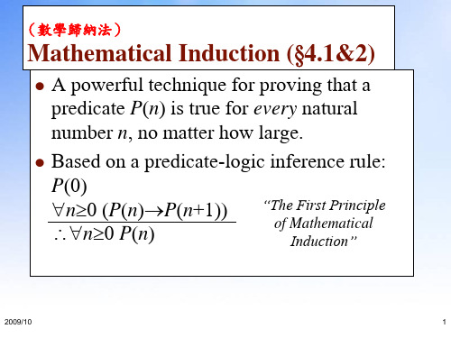
Mathematical Induction (§ 4.1&2)
A powerful technique for proving that a predicate P(n) is true for every natural number n, no matter how large. Based on a predicate-logic inference rule: P(0) “The First Principle n0 (P(n)P(n+1)) of Mathematical n0 P(n) Induction”Biblioteka 歸納假說2009/10
4
Induction Example (1st princ.)
Prove that n > 0, n < 2n. Pf. Let P(n) = (n < 2n) Basis step: P(0) = (0 < 20 = 1) = T. Inductive step: For n > 0, prove P(n)P(n+1). Assuming n < 2n, want to prove n+1 < 2n+1. Note n + 1 < 2n + 1 (根據歸納假說) < 2n + 2n (1< 2 = 220 22n-1 = 2n) = 2n+1 So n + 1 < 2n+1, and we’re done.
2009/10
1
(良序性質)
The Well-Ordering Property
The validity of the inductive inference rule can also be proved using the well-ordering property, which says: Every non-empty set of non-negative integers has a least (smallest) element. S N : mS : nS : mn 良序性質在數論上非常有用。除法公式、最大公 因數的線性表示法等,皆可直接使用良序性質得 證之。下面我們將利用良序性質來證明數學歸納 法的有效性。
- 1、下载文档前请自行甄别文档内容的完整性,平台不提供额外的编辑、内容补充、找答案等附加服务。
- 2、"仅部分预览"的文档,不可在线预览部分如存在完整性等问题,可反馈申请退款(可完整预览的文档不适用该条件!)。
- 3、如文档侵犯您的权益,请联系客服反馈,我们会尽快为您处理(人工客服工作时间:9:00-18:30)。
Rule can also be used to prove nc P(n) for a given constant cZ, where maybe c0.
In this circumstance, the base case is to prove P(c) rather than P(0), and the inductive step is to prove nc (P(n)P(n+1)).
2016/9/27
College of Computer Science & Technology, BUPT -- © Copyright Yang Juan
The Well-Ordering Property
Another way to prove the validity of the inductive inference rule is by using the wellordering property, which says that:
Do the base case (or basis step): Prove P(0). Do the inductive step: Prove n P(n)P(n+1).
E.g. you could use a direct proof, as follows: Let nN, assume P(n). (inductive hypothesis) Now, under this assumption, prove P(n+1).
2016/9/27
Induction Example (1st princ.)
Prove that the sum of the first n odd positive integers is n2. That is, prove:
n 1 : (2i 1) n
i 1
n
2
Proof by induction.
2016/9/27
College of Computer Science & Technology, BUPT -- © Copyright Yang Juan
Another 2nd Principle Example
Prove that every amount of postage of 12 cents or more can be formed using just 4cent and 5-cent stamps. P(n)=“n can be…” Base case: 12=3(4), 13=2(4)+1(5), 14=1(4)+2(5), 15=3(5), so 12n15, P(n). Inductive step: Let n15, assume 12kn P(k). Note 12n3n, so P(n3), so add a 4-cent stamp to get postage for n+1.
College of Computer Science & Technology, BUPT -- © Copyright Yang Juan
2016/9/27
The “Domino Effect”
Premise #1: Domino #0 falls. Premise #2: For every nN, if domino #n falls, then so does domino #n+1. Conclusion: All of the dominoes fall 2 down!
1 0
6
5 4 3
Note: this works even if there are infinitely many dominoes!
2016/9/27
College of Computer Science & Technology, BUPT -- © Copyright Yang Juan
Validity of Induction
n 1
(n 1)
2
2016/9/27
College of Computer Science & Technology, BUPT -- © Copyright Yang Juan
Another Induction Example
Prove that n>0, n<2n. Let P(n)=(n<2n)
The inductive inference rule then gives us n P(n).
2016/9/27
College of Computer Science & Technology, BUPT -- © Copyright Yang Juan
Generalizing Induction
2016/9/27
Example cont.
Inductive step: Prove n1: P(n)P(n+1).
Let n1, assume P(n), and prove P(n+1).
n (2i 1) (2i 1) (2(n 1) 1) i 1 i 1 By inductive 2 n 2n 1 hypothesis P(n)
A powerful, rigorous technique for proving that a predicate P(n) is true for every natural number n, no matter how large. Essentially a “domino effect” principle. Based on a predicate-logic inference rule: P(0) “The First Principle of Mathematical n0 (P(n)P(n+1)) Induction” n0 P(n)
P(n)
Base case: Let n=1. The sum of the first 1 odd positive integer is 1 which equals 12. (Cont…)
College of Computer Science & Technology, BUPT -- © Copyright Yang Juan
2016/9/27
Second Principle of Induction
A.k.a. “Strong Induction”
Characterized by another inference rule: P is true in all previous cases P(0) n0: (0kn P(k)) P(n+1) n0: P(n) The only difference between this and the 1st principle is that:
College of Computer Science & Technology, BUPT -- © Copyright Yang Juan
2016/9/27
The Method of Infinite Descent
A way to prove that P(n) is false for all nN. Sort of a converse to the principle of induction. Prove first that P(n): k<n: P(k).
Base case: P(1)=(1<21)=(1<2)=T. Inductive step: For n>0, prove P(n)P(n+1).
Assuming n<2n, prove n+1 < 2n+1. Note n + 1 < 2n + 1 (by inductive hypothesis) < 2n + 2n (because 1<2=22022n-1= 2n) = 2n+1 So n + 1 < 2n+1, and we’re done.
Induction can also be used to prove nc P(an) for any arbitrary series {an}. Can reduce these to the form already shown.
College of Computer Science & Technology, BUPT -- © Copyright Yang Juan
ห้องสมุดไป่ตู้
Basically, “For every P there is a smaller P.”
But by the well-ordering property of N, we know that P(m) P(n): P(k): n≤k.
Basically, “If there is a P, there is a smallest P.” that is, mN: ¬ P(m). There is no P.
Proof that k0 P(k) is a valid consequent:
Given any k0, the 2nd antecedent n0 (P(n)P(n+1)) trivially implies that n0 (n<k)(P(n)P(n+1)), i.e., that (P(0)P(1)) (P(1)P(2)) … (P(k1)P(k)). Repeatedly applying the hypothetical syllogism rule to adjacent implications in this list k−1 times then gives us P(0)P(k); which together with P(0) (antecedent #1) and modus ponens gives us P(k). Thus k0 P(k). ■