NUMERICAL SOLUTION of MARKOV CHAINS, p. 1–4 Comparing implicit representations of large CT
带Markov跳随机种群收获系统数值解的指数稳定性

带Markov跳随机种群收获系统数值解的指数稳定性赵朝锋;张启敏【期刊名称】《华侨大学学报(自然科学版)》【年(卷),期】2012(033)004【摘要】研究一类带跳的非线性随机种群收获动力学模型的数值解指数稳定性的问题,给出了外界环境对系统产生影响的条件下带跳的随机收获动力学系统.通过一些特殊不等式,Ito公式及Burkholder-Davis-Gundy不等式,讨论了带Markov随机种群系统数值解的收敛性,得到了数值解指数稳定所满足的充分条件,所得结论是确定性种群系统的扩展.%A harvesting exponential stability of numerical solution for nonlinear stochastic population system with jump is studied with the external environment impact on the system of Markov jump. One sufficient condition for the exponential stability of numerical solution is obtained through some special inequality, Ito formula and Burkholder-Davis-Gundy inequality. The obtained result is the expansion of certainty population system.【总页数】5页(P472-476)【作者】赵朝锋;张启敏【作者单位】北方民族大学信息与计算科学学院,宁夏银川750021;宁夏大学数学计算机学院,宁夏银川750021;北方民族大学信息与计算科学学院,宁夏银川750021【正文语种】中文【中图分类】O175.21【相关文献】1.带Markov跳的中立型随机微分方程的指数稳定性 [J], 段莹莹;张启敏2.带马尔可夫调制随机竞争种群系统数值解的指数稳定性 [J], 杜庆辉;张启敏3.带Poisson跳的随机种群扩散系统半隐式欧拉方法的数值解 [J], 马东娟;张启敏4.带Poisson跳和Markovian调制的年龄相关随机种群方程数值解的收敛性 [J], 马维军;张启敏5.带Markov跳的中立型随机微分方程的指数稳定性 [J], 段莹莹;张启敏因版权原因,仅展示原文概要,查看原文内容请购买。
马氏链方程 markov

马尔可夫链(Markov Chain)是一种数学模型,用来描述一系列事件,其中每个事件的发生只与前一个事件有关,而与之前的事件无关。
这种特性被称为“无后效性”或“马尔可夫性质”。
马尔可夫链常用于统计学、经济学、计算机科学和物理学等领域。
在统计学中,马尔可夫链被用来建模时间序列,如股票价格或天气模式。
在经济学中,马尔可夫链被用于预测经济趋势。
在计算机科学中,马尔可夫链被用于自然语言处理、图像处理和机器学习等领域。
在物理学中,马尔可夫链被用于描述粒子系统的行为。
马尔可夫链的数学表示通常是一个转移概率矩阵,该矩阵描述了从一个状态转移到另一个状态的概率。
对于给定的状态,转移概率矩阵提供了到达所有可能后续状态的概率分布。
马尔可夫链的一个关键特性是它是“齐次的”,这意味着转移概率不随时间变化。
也就是说,无论链在何时处于特定状态,从该状态转移到任何其他状态的概率都是相同的。
马尔可夫链的方程通常表示为:P(X(t+1) = j | X(t) = i) = p_ij其中,X(t)表示在时间t的链的状态,p_ij表示从状态i转移到状态j的概率。
这个方程描述了马尔可夫链的核心特性,即未来的状态只与当前状态有关,而与过去状态无关。
马尔可夫链的一个重要应用是在蒙特卡罗方法中,特别是在马尔可夫链蒙特卡罗(MCMC)方法中。
MCMC 方法通过构造一个满足特定条件的马尔可夫链来生成样本,从而估计难以直接计算的统计量。
这些样本可以用于估计函数的期望值、计算积分或进行模型选择等任务。
总之,马尔可夫链是一种强大的工具,用于建模和预测一系列相互关联的事件。
通过转移概率矩阵和马尔可夫链方程,可以描述和分析这些事件的行为和趋势。
马尔科夫过程介绍
A vector with nonnegative entries that add up to 1 is called a probability vector. A stochastic matrix is a square matrix whose columns are probability vectors. A Markov chain is a sequence of probability vectors x0, x1, x2, …, together with a stochastic matrix P, such that
For example, if the population of a city and its suburbs were measured each year, then a vector such as
0.60
x0
0.40
could indicate that 60% of the population lives in the city and
So the population distribution could be
Similarly, the distribution in 2019 is described by a vector x2, where
What is Markov matrix?
An nxn matrix whose form satisfies two properties below 1.All entries ≥0; 2.All columns add to 1; is called a Markov matrix. Such as
Advanced Mathematical Modeling Techniques
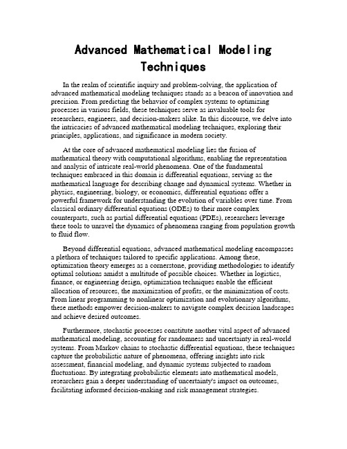
Advanced Mathematical ModelingTechniquesIn the realm of scientific inquiry and problem-solving, the application of advanced mathematical modeling techniques stands as a beacon of innovation and precision. From predicting the behavior of complex systems to optimizing processes in various fields, these techniques serve as invaluable tools for researchers, engineers, and decision-makers alike. In this discourse, we delve into the intricacies of advanced mathematical modeling techniques, exploring their principles, applications, and significance in modern society.At the core of advanced mathematical modeling lies the fusion of mathematical theory with computational algorithms, enabling the representation and analysis of intricate real-world phenomena. One of the fundamental techniques embraced in this domain is differential equations, serving as the mathematical language for describing change and dynamical systems. Whether in physics, engineering, biology, or economics, differential equations offer a powerful framework for understanding the evolution of variables over time. From classical ordinary differential equations (ODEs) to their more complex counterparts, such as partial differential equations (PDEs), researchers leverage these tools to unravel the dynamics of phenomena ranging from population growth to fluid flow.Beyond differential equations, advanced mathematical modeling encompasses a plethora of techniques tailored to specific applications. Among these, optimization theory emerges as a cornerstone, providing methodologies to identify optimal solutions amidst a multitude of possible choices. Whether in logistics, finance, or engineering design, optimization techniques enable the efficient allocation of resources, the maximization of profits, or the minimization of costs. From linear programming to nonlinear optimization and evolutionary algorithms, these methods empower decision-makers to navigate complex decision landscapes and achieve desired outcomes.Furthermore, stochastic processes constitute another vital aspect of advanced mathematical modeling, accounting for randomness and uncertainty in real-world systems. From Markov chains to stochastic differential equations, these techniques capture the probabilistic nature of phenomena, offering insights into risk assessment, financial modeling, and dynamic systems subjected to random fluctuations. By integrating probabilistic elements into mathematical models, researchers gain a deeper understanding of uncertainty's impact on outcomes, facilitating informed decision-making and risk management strategies.The advent of computational power has revolutionized the landscape of advanced mathematical modeling, enabling the simulation and analysis of increasingly complex systems. Numerical methods play a pivotal role in this paradigm, providing algorithms for approximating solutions to mathematical problems that defy analytical treatment. Finite element methods, finite difference methods, and Monte Carlo simulations are but a few examples of numerical techniques employed to tackle problems spanning from structural analysis to option pricing. Through iterative computation and algorithmic refinement, these methods empower researchers to explore phenomena with unprecedented depth and accuracy.Moreover, the interdisciplinary nature of advanced mathematical modeling fosters synergies across diverse fields, catalyzing innovation and breakthroughs. Machine learning and data-driven modeling, for instance, have emerged as formidable allies in deciphering complex patterns and extracting insights from vast datasets. Whether in predictive modeling, pattern recognition, or decision support systems, machine learning algorithms leverage statistical techniques to uncover hidden structures and relationships, driving advancements in fields as diverse as healthcare, finance, and autonomous systems.The application domains of advanced mathematical modeling techniques are as diverse as they are far-reaching. In the realm of healthcare, mathematical models underpin epidemiological studies, aiding in the understanding and mitigation of infectious diseases. From compartmental models like the SIR model to agent-based simulations, these tools inform public health policies and intervention strategies, guiding efforts to combat pandemics and safeguard populations.In the domain of climate science, mathematical models serve as indispensable tools for understanding Earth's complex climate system and projecting future trends. Coupling atmospheric, oceanic, and cryospheric models, researchers simulate the dynamics of climate variables, offering insights into phenomena such as global warming, sea-level rise, and extreme weather events. By integrating observational data and physical principles, these models enhance our understanding of climate dynamics, informing mitigation and adaptation strategies to address the challenges of climate change.Furthermore, in the realm of finance, mathematical modeling techniques underpin the pricing of financial instruments, the management of investment portfolios, and the assessment of risk. From option pricing models rooted in stochastic calculus to portfolio optimization techniques grounded in optimization theory, these tools empower financial institutions to make informed decisions in a volatile and uncertain market environment. By quantifying risk and return profiles, mathematical models facilitate the allocation of capital, the hedging of riskexposures, and the management of investment strategies, thereby contributing to financial stability and resilience.In conclusion, advanced mathematical modeling techniques represent a cornerstone of modern science and engineering, providing powerful tools for understanding, predicting, and optimizing complex systems. From differential equations to optimization theory, from stochastic processes to machine learning, these techniques enable researchers and practitioners to tackle a myriad of challenges across diverse domains. As computational capabilities continue to advance and interdisciplinary collaborations flourish, the potential for innovation and discovery in the realm of mathematical modeling knows no bounds. By harnessing the power of mathematics, computation, and data, we embark on a journey of exploration and insight, unraveling the mysteries of the universe and shaping the world of tomorrow.。
markovchains 马尔科夫链PPT课件

Estimating the Model Parameters
• given some data (e.g. a set of sequences from CpG islands), how can we determine the probability parameters of our model?
Markov Chain Models
BMI/CS 576
Fall 2010
Motivation for Markov Models in Computational Biology
• there are many cases in which we would like to represent the statistical regularities of some class of sequences – genes – various regulatory sites in DNA (e.g., where RNA polymerase and transcription factors bind) – proteins in a given family
• can also have an end state; allows the model to represent – a distribution over sequences of different lengths – preferences for ending sequences with certain symbols
is n o t s u p p o r te d
where
M acintosh PICT im age form at is not supported
represents the
信息论英文课后部分习题答案
本答案是英文原版的配套答案,与翻译的中文版课本题序不太一样但内容一样。
翻译的中文版增加了题量。
2.2、Entropy of functions. Let X be a random variable taking on a finite number of values. What is the (general) inequality relationship of ()H X and ()H Y if(a) 2X Y =?(b) cos Y X =?Solution: Let ()y g x =. Then():()()x y g x p y p x ==∑.Consider any set of x ’s that map onto a single y . For this set()():():()()log ()log ()log ()x y g x x y g x p x p x p x p y p y p y ==≤=∑∑,Since log is a monotone increasing function and ():()()()x y g x p x p x p y =≤=∑.Extending this argument to the entire range of X (and Y ), we obtain():()()log ()()log ()x y x g x H X p x p x p x p x =-=-∑∑∑()log ()()yp y p y H Y ≥-=∑,with equality iff g if one-to-one with probability one.(a) 2X Y = is one-to-one and hence the entropy, which is just a function of the probabilities does not change, i.e., ()()H X H Y =.(b) cos Y X =is not necessarily one-to-one. Hence all that we can say is that ()()H X H Y ≥, which equality if cosine is one-to-one on the range of X .2.16. Example of joint entropy. Let (,)p x y be given byFind(a) ()H X ,()H Y .(b) (|)H X Y ,(|)H Y X . (c) (,)H X Y(d) ()(|)H Y H Y X -.(e) (;)I X Y(f) Draw a Venn diagram for the quantities in (a) through (e).Solution:Fig. 1 Venn diagram(a) 231()log log30.918 bits=()323H X H Y =+=.(b) 12(|)(|0)(|1)0.667 bits (/)33H X Y H X Y H X Y H Y X ==+===((,)(|)()p x y p x y p y =)((|)(,)()H X Y H X Y H Y =-)(c) 1(,)3log3 1.585 bits 3H X Y =⨯=(d) ()(|)0.251 bits H Y H Y X -=(e)(;)()(|)0.251 bits=-=I X Y H Y H Y X(f)See Figure 1.2.29 Inequalities. Let X,Y and Z be joint random variables. Prove the following inequalities and find conditions for equality.(a) )ZHYXH≥X(Z()|,|(b) )ZIYXI≥X((Z);,;(c) )XYXHZ≤Z-H-XYH),(,)(((X,,)H(d) )XYIZIZII+-XZY≥Y(););(|;;(Z|)(XSolution:(a)Using the chain rule for conditional entropy,HZYXHZXH+XH≥XYZ=),(|(Z)(||,()|)With equality iff 0YH,that is, when Y is a function of X andXZ,|(=)Z.(b)Using the chain rule for mutual information,ZIXXIZYX+=,I≥IYZ(|;)X);)(,;;(Z)(With equality iff 0ZYI, that is, when Y and Z areX)|;(=conditionally independent given X.(c)Using first the chain rule for entropy and then definition of conditionalmutual information,XZHYHIXZYX==-H-XHYYZ)()(;Z)|,|),|(X(,,)(XHXZH-Z≤,=,)()()(X|HWith equality iff 0ZYI, that is, when Y and Z areX(=|;)conditionally independent given X .(d) Using the chain rule for mutual information,);()|;();,();()|;(Z X I X Y Z I Z Y X I Y Z I Y Z X I +==+And therefore this inequality is actually an equality in all cases.4.5 Entropy rates of Markov chains.(a) Find the entropy rate of the two-state Markov chain with transition matrix⎥⎦⎤⎢⎣⎡--=1010010111p p p p P (b) What values of 01p ,10p maximize the rate of part (a)?(c) Find the entropy rate of the two-state Markov chain with transition matrix⎥⎦⎤⎢⎣⎡-=0 1 1p p P(d) Find the maximum value of the entropy rate of the Markov chain of part (c). We expect that the maximizing value of p should be less than 2/1, since the 0 state permits more information to be generated than the 1 state.Solution:(a) T he stationary distribution is easily calculated.10010*********,p p p p p p +=+=ππ Therefore the entropy rate is10011001011010101012)()()()()|(p p p H p p H p p H p H X X H ++=+=ππ(b) T he entropy rate is at most 1 bit because the process has only two states. This rate can be achieved if( and only if) 2/11001==p p , in which case the process is actually i.i.d. with2/1)1Pr()0Pr(====i i X X .(c) A s a special case of the general two-state Markov chain, the entropy rate is1)()1()()|(1012+=+=p p H H p H X X H ππ.(d) B y straightforward calculus, we find that the maximum value of)(χH of part (c) occurs for 382.02/)53(=-=p . The maximum value isbits 694.0)215()1()(=-=-=H p H p H (wrong!)5.4 Huffman coding. Consider the random variable⎪⎪⎭⎫ ⎝⎛=0.02 0.03 0.04 0.04 0.12 0.26 49.0 7654321x x x x x x x X (a) Find a binary Huffman code for X .(b) Find the expected codelength for this encoding.(c) Find a ternary Huffman code for X .Solution:(a) The Huffman tree for this distribution is(b)The expected length of the codewords for the binary Huffman code is 2.02 bits.( ∑⨯=)()(i p l X E )(c) The ternary Huffman tree is5.9 Optimal code lengths that require one bit above entropy. The source coding theorem shows that the optimal code for a random variable X has an expected length less than 1)(+X H . Given an example of a random variable for which the expected length of the optimal code is close to 1)(+X H , i.e., for any 0>ε, construct a distribution for which the optimal code has ε-+>1)(X H L .Solution: there is a trivial example that requires almost 1 bit above its entropy. Let X be a binary random variable with probability of 1=X close to 1. Then entropy of X is close to 0, but the length of its optimal code is 1 bit, which is almost 1 bit above its entropy.5.25 Shannon code. Consider the following method for generating a code for a random variable X which takes on m values {}m ,,2,1 with probabilities m p p p ,,21. Assume that the probabilities are ordered so thatm p p p ≥≥≥ 21. Define ∑-==11i k i i p F , the sum of the probabilities of allsymbols less than i . Then the codeword for i is the number ]1,0[∈i Frounded off to i l bits, where ⎥⎥⎤⎢⎢⎡=i i p l 1log . (a) Show that the code constructed by this process is prefix-free and the average length satisfies 1)()(+<≤X H L X H .(b) Construct the code for the probability distribution (0.5, 0.25, 0.125, 0.125).Solution:(a) Since ⎥⎥⎤⎢⎢⎡=i i p l 1log , we have 11log 1log +<≤i i i p l pWhich implies that 1)()(+<=≤∑X H l p L X H i i .By the choice of i l , we have )1(22---<≤ii l i l p . Thus j F , i j > differs from j F by at least il -2, and will therefore differ from i F is at least one place in the first i l bits of the binary expansion of i F . Thus thecodeword for j F , i j >, which has length i j l l ≥, differs from thecodeword for i F at least once in the first i l places. Thus no codewordis a prefix of any other codeword.(b) We build the following table3.5 AEP. Let ,,21X X be independent identically distributed random variables drawn according to theprobability mass function {}m x x p ,2,1),(∈. Thus ∏==n i i n x p x x x p 121)(),,,( . We know that)(),,,(log 121X H X X X p n n →- in probability. Let ∏==n i i n x q x x x q 121)(),,,( , where q is another probability mass function on {}m ,2,1.(a) Evaluate ),,,(log 1lim 21n X X X q n-, where ,,21X X are i.i.d. ~ )(x p . Solution: Since the n X X X ,,,21 are i.i.d., so are )(1X q ,)(2X q ,…,)(n X q ,and hence we can apply the strong law of large numbers to obtain∑-=-)(log 1lim ),,,(log 1lim 21i n X q n X X X q n 1..))((log p w X q E -=∑-=)(log )(x q x p∑∑-=)(log )()()(log )(x p x p x q x p x p )()||(p H q p D +=8.1 Preprocessing the output. One is given a communication channel withtransition probabilities )|(x y p and channel capacity );(max )(Y X I C x p =.A helpful statistician preprocesses the output by forming )(_Y g Y =. He claims that this will strictly improve the capacity.(a) Show that he is wrong.(b) Under what condition does he not strictly decrease the capacity? Solution:(a) The statistician calculates )(_Y g Y =. Since _Y Y X →→ forms a Markov chain, we can apply the data processing inequality. Hence for every distribution on x ,);();(_Y X I Y X I ≥. Let )(_x p be the distribution on x that maximizes );(_Y X I . Then__)()()(_)()()();(max );();();(max __C Y X I Y X I Y X I Y X I C x p x p x p x p x p x p ==≥≥===.Thus, the statistician is wrong and processing the output does not increase capacity.(b) We have equality in the above sequence of inequalities only if we have equality in data processing inequality, i.e., for the distribution that maximizes );(_Y X I , we have Y Y X →→_forming a Markov chain.8.3 An addition noise channel. Find the channel capacity of the following discrete memoryless channel:Where {}{}21Pr 0Pr ====a Z Z . The alphabet for x is {}1,0=X . Assume that Z is independent of X . Observe that the channel capacity depends on the value of a . Solution: A sum channel.Z X Y += {}1,0∈X , {}a Z ,0∈We have to distinguish various cases depending on the values of a .0=a In this case, X Y =,and 1);(max =Y X I . Hence the capacity is 1 bitper transmission.1,0≠≠a In this case, Y has four possible values a a +1,,1,0. KnowingY ,we know the X which was sent, and hence 0)|(=Y X H . Hence thecapacity is also 1 bit per transmission.1=a In this case Y has three possible output values, 0,1,2, the channel isidentical to the binary erasure channel, with 21=f . The capacity of this channel is 211=-f bit per transmission.1-=a This is similar to the case when 1=a and the capacity is also 1/2 bit per transmission.8.5 Channel capacity. Consider the discrete memoryless channel)11 (mod Z X Y +=, where ⎪⎪⎭⎫ ⎝⎛=1/3 1/3, 1/3,3 2,,1Z and {}10,,1,0 ∈X . Assume thatZ is independent of X .(a) Find the capacity.(b) What is the maximizing )(*x p ?Solution: The capacity of the channel is );(max )(Y X I C x p =)()()|()()|()();(Z H Y H X Z H Y H X Y H Y H Y X I -=-=-=bits 311log)(log );(=-≤Z H y Y X I , which is obtained when Y has an uniform distribution, which occurs when X has an uniform distribution.(a)The capacity of the channel is bits 311log /transmission.(b) The capacity is achieved by an uniform distribution on the inputs.10,,1,0for 111)( ===i i X p 8.12 Time-varying channels. Consider a time-varying discrete memoryless channel. Let n Y Y Y ,,21 be conditionally independent givenn X X X ,,21 , with conditional distribution given by ∏==ni i i i x y p x y p 1)|()|(.Let ),,(21n X X X X =, ),,(21n Y Y Y Y =. Find );(max )(Y X I x p . Solution:∑∑∑∑∑=====--≤-≤-=-=-=-=ni i n i i i n i i ni i i ni i i n p h X Y H Y H X Y H Y H X Y Y Y H Y H X Y Y Y H Y H X Y H Y H Y X I 111111121))(1()|()()|()(),,|()()|,,()()|()();(With equlity ifnX X X ,,21 is chosen i.i.d. Hence∑=-=ni i x p p h Y X I 1)())(1();(max .10.2 A channel with two independent looks at Y . Let 1Y and 2Y be conditionally independent and conditionally identically distributed givenX .(a) Show );();(2),;(21121Y Y I Y X I Y Y X I -=. (b) Conclude that the capacity of the channelX(Y1,Y2)is less than twice the capacity of the channelXY1Solution:(a) )|,(),(),;(212121X Y Y H Y Y H Y Y X I -=)|()|();()()(212121X Y H X Y H Y Y I Y H Y H ---+=);();(2);();();(2112121Y Y I Y X I Y Y I Y X I Y X I -=-+=(b) The capacity of the single look channel 1Y X → is );(max 1)(1Y X I C x p =.Thecapacityof the channel ),(21Y Y X →is11)(211)(21)(22);(2max );();(2max ),;(max C Y X I Y Y I Y X I Y Y X I C x p x p x p =≤-==10.3 The two-look Gaussian channel. Consider the ordinary Shannon Gaussian channel with two correlated looks at X , i.e., ),(21Y Y Y =, where2211Z X Y Z X Y +=+= with a power constraint P on X , and ),0(~),(221K N Z Z ,where⎥⎦⎤⎢⎣⎡=N N N N K ρρ. Find the capacity C for (a) 1=ρ (b) 0=ρ (c) 1-=ρSolution:It is clear that the two input distribution that maximizes the capacity is),0(~P N X . Evaluating the mutual information for this distribution,),(),()|,(),()|,(),(),;(max 212121212121212Z Z h Y Y h X Z Z h Y Y h X Y Y h Y Y h Y Y X I C -=-=-==Nowsince⎪⎪⎭⎫⎝⎛⎥⎦⎤⎢⎣⎡N N N N N Z Z ,0~),(21ρρ,wehave)1()2log(21)2log(21),(222221ρππ-==N e Kz e Z Z h.Since11Z X Y +=, and22Z X Y +=, wehave ⎪⎪⎭⎫⎝⎛⎥⎦⎤⎢⎣⎡++++N N P N N P N Y Y P P ,0~),(21ρρ, And ))1(2)1(()2log(21)2log(21),(222221ρρππ-+-==PN N e K e Y Y h Y .Hence⎪⎪⎭⎫⎝⎛++=-=)1(21log 21),(),(21212ρN P Z Z h Y Y h C(a) 1=ρ.In this case, ⎪⎭⎫⎝⎛+=N P C 1log 21, which is the capacity of a single look channel.(b) 0=ρ. In this case, ⎪⎭⎫⎝⎛+=N P C 21log 21, which corresponds to using twice the power in a single look. The capacity is the same as the capacity of the channel )(21Y Y X +→.(c) 1-=ρ. In this case, ∞=C , which is not surprising since if we add1Y and 2Y , we can recover X exactly.10.4 Parallel channels and waterfilling. Consider a pair of parallel Gaussianchannels,i.e.,⎪⎪⎭⎫⎝⎛+⎪⎪⎭⎫ ⎝⎛=⎪⎪⎭⎫ ⎝⎛212121Z Z X X Y Y , where⎪⎪⎭⎫ ⎝⎛⎥⎥⎦⎤⎢⎢⎣⎡⎪⎪⎭⎫ ⎝⎛222121 00 ,0~σσN Z Z , And there is a power constraint P X X E 2)(2221≤+. Assume that 2221σσ>. At what power does the channel stop behaving like a single channel with noise variance 22σ, and begin behaving like a pair of channels? Solution: We will put all the signal power into the channel with less noise until the total power of noise+signal in that channel equals the noise power in the other channel. After that, we will split anyadditional power evenly between the two channels. Thus the combined channel begins to behave like a pair of parallel channels when the signal power is equal to the difference of the two noise powers, i.e., when 22212σσ-=P .。
马尔科夫计算例题

马尔科夫计算例题
马尔科夫链蒙特卡洛(Markov Chain Monte Carlo,MCMC)是一种统计模拟方法,用于从复杂的分布中抽样。
以下是一个简单的马尔科夫链蒙特卡洛计算例题:
假设我们有一个随机变量 \(X\),其分布是 \(P(X)\)。
我们的目标是计算
\(P(X)\) 的期望值,也就是:
\(\text{E}[X] = \int x P(x) dx\)
但是,直接计算这个积分是非常困难的。
因此,我们使用马尔科夫链蒙特卡洛方法来近似这个积分。
步骤如下:
1. 初始化一个随机数 \(x_0\) 作为当前状态。
2. 生成一个随机数 \(r\) 服从均匀分布 \(U(0,1)\)。
3. 计算接受率 \(A = \min(1, \frac{P(x_i)}{P(x_j)})\),其中 \(j\) 是 \(r\) 落入的区间中的状态。
4. 以概率 \(A\) 接受 \(x_j\) 作为新的状态 \(x_{i+1}\)。
5. 如果接受,回到步骤 2;否则,令 \(i = i+1\) 并回到步骤 2。
6. 重复步骤 2-5,直到达到足够的样本数量。
然后,我们可以用这些样本的平均值来近似期望值。
这是一个简单的例子,实际上马尔科夫链蒙特卡洛方法可以用于更复杂的问题,如高维积分、优化问题等。
几类非负矩阵特征值反问题

The Inverse Eigenvalue Problem for Several Classes of Nonnegative MatricesA DissertationSubmitted for the Degree of MasterOn computational mathematicsby Tian YuUnder the Supervision ofProf. Wang Jinlin(College of Mathematics and Information Sciences)Nanchang Hangkong University, Nanchang, ChinaJune, 2011摘 要非负矩阵理论一直是矩阵理论中最活跃的研究领域之一,在数学、自然科学的其他分支以及社会科学中都广泛涉及到,例如博弈论、Markov链(随机矩阵)、概率论、概率算法、数值分析、离散分布、群论、matrix scaling、小振荡弹性系统(振荡矩阵)和经济学等等.近年来,特征值反问题是矩阵理论研究的热点,本文将就非负矩阵特征值反问题(NIEP)这一问题进行研究.文章主要研究几类特殊形式的非负矩阵特征值反问题,得到了相关问题的充分必要条件和一些充分条件,进而给出了这几类特殊形式的非负矩阵特征值反问题数值算法,并通过数值算例来验证相关定理的正确性以及算法的准确性.主要工作如下: 第一章是绪论部分,阐述了非负矩阵特征值反问题的重要意义和发展历程,介绍国内外研究现状.第二章,研究非负三对角矩阵特征值反问题.首先对三阶非负三对角矩阵特征值反问题,分几种情形进行讨论,解决了三阶非负三对角矩阵特征值反问题,得到了三阶非负三对角矩阵特征值反问题有解的充分必要条件.然后对n阶非负三对角矩阵特征值反问题,通过非负三对角矩阵截断矩阵特征多项式,并结合Jacobi 矩阵特征值的关系,得到了非负三对角矩阵的特征值的相关性质,并最终解决了非负三对角矩阵特征值反问题.第三章,研究非负五对角矩阵特征值反问题.三阶非负五对角矩阵,即是三阶非负矩阵,文中给出了其特征值反问题有解的充分必要条件,而对于n阶非负五对角矩阵特征值反问题,由于其复杂性,文中仅给出了它的一些充分条件.第四章,研究非负循环矩阵特征值反问题.首先总结了NIEP近些年来取得的研究成果,提出实循环矩阵特征值反问题,并成功解决了实循环矩阵特征值反问题,得到其充分必要条件.最后在实循环矩阵特征值反问题的基础上提出非负循环矩阵特征值反问题,得到了充分条件和相关推论.第五章,根据第二、三、四章的结论给出相关算法和实例.第六章,在总结全文的同时,提出了需要进一步研究的问题.关键词:特征值,反问题,非负三对角矩阵,非负五对角矩阵,非负循环矩阵AbstractThe theory of nonnegative matrices has always been one of the most active research areas in the matrix theory and has been widely applied in mathematics and other branches of natural and social sciences. There are, for example, game theory, Markov chains (stochastic martices), theory of probability, probabilistic algorithms, numerical analysis, discrete distribution, group theory, matrix scaling, theory of small osillations of elastic systems (oscillation marrices), economics and so on. In recent years, the inverse eigenvalue problem comes to be the focus of the matrix theory. This thesis will study the inverse eigenvalue problem for nonnegative matrices (NIEP). The major researches of this theisis focus on the inverse eigenvalue problem for several special classes of nonnegative matrices, the necessary and sufficient conditions and some sufficient conditions of which are derived. Moreover, the numerical algorithms of the inverse eigenvalue problem for these special classes of nonnegative matrices are given, the accuracy of which together with the correcteness of related theories is testified by several numerical examples. The main procedures of this theisis are as follows:In the first chapter, the significance and the development of the inverse eigenvalue problem for nonnegative matrices are addressed, and the research situation home and abroad is introduced.In the second chapter, the inverse eigenvalue problem for nonnegative tridiagonal matrices is studied. First, the inverse eigenvalue problem for 33⨯ nonnegative tridiagonal matrices is solved by discussion of a variety of situations. Moveover ,the necessary and sufficient conditions of the solutions of the inverse eigenvalue problem for 33⨯ nonnegative tridiagonal matrices are derived. Then, the properties of eigenvalue of n n ⨯ nonnegative tridiagonal matrices are derived by characteristic polynomial of truncated matrices of nonnegative tridiagonal matrices, with the combination of the relationship between eigenvalues of Jacobi matrix. Finally, the inverse eigenvalue problem for nonnegative tridiagonal matrices is solved.In the third chapter, the inverse eigenvalue problem for nonnegative five-diagonal matrices is studied. 33⨯ nonnegative five-diagonal matrices is also 33⨯ nonnegative matrices, the necessary and sufficient conditions of the solutions of the inverse eigenvalue problem for which are given in this thesis. For the inverseeigenvalue problem for n nnonnegative five-diagonal matrices, only some sufficient conditions are given because of its complexity.In the fourth chapter, the inverse eigenvalue problem for nonnegative circulant matrices is studied. First, some remarkable conclusions of the inverse eigenvalue problem for nonnegative matrices in recent years are summarized. Then, the inverse eigenvalue problem for real circulant matrices is advanced and successfully solved, the necessary and sufficient conditions of which are given also. Finally, the inverse eigenvalue problem for nonnegative circulant matrices is advanced based on the inverse eigenvalue problem for real circulant matrices, whose sufficient conditions and some relevant conclusions are given.In the fifth chapter, some algorithms and numerical examples are given based on the conclusions derived in the previous three chapters.In the sixth chapter, the summary of the paper is given and the future research work is put forward.Key words: eigenvalue, inverse problem, nonnegative tridiagonal matrices, nonnegative five-diagonal matrices, nonnegative circulant matrices目录第一章 绪论 (1)1.1选题的依据与意义 (1)1.2非负矩阵特征值反问题的研究现状 (2)1.3研究的主要内容 (3)第二章 非负三对角矩阵特征值反问题 (5)2.1引言 (5)2.2三阶非负三对角矩阵特征值反问题 (6)n阶非负三对角矩阵特征值反问题 (24)2.3第三章 非负五对角矩阵特征值反问题 (33)3.1引言 (33)3.2非负五对角矩阵特征值反问题相关结论 (33)第四章 非负循环矩阵特征值反问题 (38)4.1引言 (38)4.2一类特殊矩阵的特征值反问题 (40)4.3非负循环矩阵特征值反问题 (42)第五章 算法设计及实例 (45)5.1非负三对角矩阵特征值反问题算法 (45)5.2非负五对角矩阵特征值反问题算法 (47)5.3实循环矩阵特征值反问题算法 (49)5.4非负循环矩阵特征值反问题算法 (50)第六章 总结与展望 (53)6.1全文总结 (53)6.2工作展望 (53)参考文献 (54)攻读硕士学位期间发表的论文 (57)致 谢 (58)IV第一章 绪论1.1 选题的依据与意义反问题,顾名思义是相对于正问题而言的,它是根据事物的演化结果,由可观测的现象来探求事物的内部规律或所受的外部影响,由表及里,索隐探秘.在数学中有着许多反问题,例如已知两个自然数的乘积,如何求这两个自然数;已知导数,如何求原函数;已知一个角的三角函数值,如何求这个角的度数,等等.近些年来,人们在生活、工业生产、科学探索中经常遇到反问题,对反问题的研究也越来越受到重视.事实上,对于一般问题来说,反问题要比正问题复杂.如前面提到的求角度数问题,已知一个角,求其三角函数值是唯一的,但如果只知道一个角的三角函数值而不对这个角加以约束,这样的角将会有无穷多个,因而反问题的解一般来说不唯一.另外,反问题的解也极不稳定.因此,对反问题的研究主要包括以下几个方面:存在性、唯一性、稳定性、数值方法和实际应用.矩阵特征值反问题(又称代数特征值反问题或逆特征值问题),就是根据已给定的特征值和/或特征向量等信息来确定一个矩阵,使得该矩阵满足所给的条件.矩阵特征值反问题的来源非常广泛.它不仅来自于数学物理反问题的离散化,而且来自固体力学、粒子物理、量子物理、结构设计、系统参数识别、自动控制等许多领域.由于矩阵特征值反问题的应用广泛性,因而自从此类问题被提出来的几十年里,受到了大量学者的深入研究,得到了一系列优秀成果.本文研究的非负矩阵特征值反问题正是在此期间提出来的,它作为矩阵特征值反问题的一个重要分支,尤其是在概率统计、随机分布、系统分析方面有着重要应用.所谓非负矩阵特征值反问题就是根据已给定的特征值信息来确定一个非负矩阵,使得该非负矩阵满足所给的条件.例如在概率统计中提出一类随机矩阵(矩阵的元素行和为1),这类矩阵在Markov链中有着重要应用,假如对矩阵的特征值有某些特殊要求,能否构造和如何构造出此类矩阵?非负矩阵特征值反问题从提出到现在的几十年间,虽然受到了大量学者的研究,但由于其复杂性,目前仍存在大量的疑难问题尚未解决,这也是它吸引众多学者研究的魅力所在.因而从以上可以看出对非负矩阵特征值的研究无论是对数学本身的发展还是对其它科学的发展都有着重要的意义及广阔的前景.1.2 非负矩阵特征值反问题的研究现状非负矩阵特征值反问题的提出始于上个世纪50年代,它是由矩阵特征值反问题抽离出来的一个子问题.1937年,Kolmogorov [1]首先提出了给定一个复数z 何时为某个非负矩阵特征值的问题.1949年,Suleimanova [2]扩展了Kolmogorov 提出的问题,称为非负矩阵特征值反问题(简称NIEP),即寻找以一组复数12{,,,}n σλλλ= 为特征值的n 阶非负矩阵A ,并且假若能够找到这样一个矩阵A ,就说矩阵A 实现了σ.Kolmogorov 问题显然很容易回答,Minc [3]给出了解答,即对于33⨯阶正循环矩阵,总可以找到一个这样的矩阵使得给定的复数z 作为它的特征值.然而NIEP 从提出至今仍未得到很好地解决,为此一些学者首先从NIEP 的必要条件开始研究.Loewy 和Londow [4]、Johnson [5]给出文献[6]中NIEP 的四个必要条件,其中最后一个条件称为JLL 条件.1998年,Laffey 和Meehan [7]又对奇数阶非负矩阵进行了讨论,给出了奇数阶非负矩阵迹为零的JLL 条件.由于一般的n 阶NIEP 无法直接解答,一批学者考虑了低阶矩阵的情形.1978年,Loewy 和Londow [4]完全解决3n =时的NIEP,给出了四个充分必要条件.45n =、时的NIEP,目前只解决了迹为零的情形.1996年,Reams [8]解决了4n =时迹为零的情形,即:令1234{,,,}σλλλλ=为一组复数,假若120,0,S S =≥30S ≥和2244S S ≤(这里的41k k i i S λ==∑),则必存在一个4阶非负矩阵能够实现σ.1999年,Laffey 和Meehan [9]解决了5n =时迹为零的情形.上面介绍了6n <的情形,然而当6n ≥时,NIEP 却是一个极大地挑战,到目前为止,未见任何形式的解答.虽然NIEP 未曾从正面给出很好的解答,但却吸引大批学者对12{,,}n σλλλ= ,的特殊形式作出深入探讨,这其中包括H.Suleimanova、H.Perfect、R.Kellogg、Salzman、Guo Wuwen 等等.Suleimanova [2]证明0(2,3,,)i i n λ≤= 的σ可被实现的充分必要条件是10ni i λ=≥∑.Kellogg [10]对σ的序列进行分块研究,给出了某些符合要求的分块可被实现.Guo Wuwen [11-12]对已可实现的σ修正做了研究,其中修正后可被实现与σ中最大的数有着密切关系,文献[12]定理3.1的结论尤为重要,它在研究扩展σ可被实现中被广泛引用.另外值得一提的是Ricardo.Soto、Alberto.Borobia、Julio.Moro 三位近十年来在非负矩阵特征值反问题上做了大量深入的研究,文献[13-18]集中反映了他们在这一块的研究成果.上面介绍了NIEP,如果把上面的非负矩阵换成非负对称矩阵,则称为非负对称矩阵特征值反问题(简称SNIEP);如果把上面的一组复数12{,,}n σλλλ= ,换成一组实数,则称为非负矩阵实特征值反问题(简称RNIEP).SNIEP和RNIEP都是NIEP的子问题,它们是研究NIEP的重要组成部分,虽然两者研究的都是实特征值,但它们并不完全等价.一般地,当5n≥时,这是两个完全不同的问题.目前,当4n≤时,SNIEP已被完全解决,当5n=时,R.Loewy和J.J.Mcdonald在文献[9]中做了详细的讨论.而当6n≥时,尚无人解决.文献[19-21]给出了SNIEP的相关结论.4n=时的RNIEP已被解决,事实上,Loewy和Londow在文献[4]中给出的NIEP四个必要条件也是4阶RNIEP的充分条件.当5n≥时,目前尚未有所突破.另外,文献[2,10,22,23,24,25]给出了RNIEP的相关结论.随机矩阵和双随机矩阵作为非负矩阵的两种特殊形式,在研究NIEP中有着极为重要的应用,这里把它们归为一类问题,即随机和双随机矩阵特征值反问题.Johnson[26]证明了如果一个非负矩阵A有正Perron根ρ,则存在一个随机矩阵与1Aρ同谱.1981年,Soules[27]给出了一种构造对称双随机矩阵的方法并得到构造对称双随机矩阵的充分条件.以上是NIEP的主要研究的方向,由于NIEP的复杂性和作者的水平限度,可能衍生出更多的小问题,本文没有一一涉及到,在此后面将不再叙述.此外,由于NIEP研究不够成熟,关于它的数值计算目前研究的不多.Robert.Orsi[28]利用交错射影的思想构造出一种迭代方法来计算非负矩阵特征值反问题,但需指出的是这种迭代并不一定会能得出好的结果,仍需要找到好的判定条件.O.Rojo等在文献[29-30]中通过快速Fourier变化巧妙地得到一种构造对称非负矩阵的方法,大大节省计算时间,这种方法通过在Matlab上实现,证明效率是非常高的.目前,国内尚无对此方面的研究的相关文献.从以上可以看出,虽然非负矩阵特征值反问题的研究得到了一定的成果,但仍有大量的问题需要解决,本文将从几类特殊矩阵来探讨此类问题,进一步促进此方向的研究.例如:能否给出非负(对称)三对角矩阵的特征值反问题的充要条件以及如何实现?如何实现非负循环矩阵的特征值反问题?等等.1.3 研究的主要内容本文研究几类特殊形式的非负矩阵特征值反问题,得到了相关问题的充分必要条件和一些充分条件,进而给出这几种特殊形式的非负矩阵特征值反问题算法,并通过数值算例来验证相关定理的正确性以及算法的准确性.主要工作如下:第一章是绪论部分,阐述了非负矩阵特征值反问题的重要意义和发展历程,介绍国内外研究现状.第二章,研究非负三对角矩阵特征值反问题.首先对三阶非负三对角矩阵特征值反问题,分几种情形进行讨论,解决了三阶非负三对角矩阵特征值反问题,得到了三阶非负三对角矩阵特征值反问题有解的充分必要条件.然后对n阶非负三对角矩阵特征值反问题,通过非负三对角矩阵截断矩阵特征多项式,并结合Jacobi矩阵特征值的关系,得到了非负三对角矩阵的特征值的相关性质,并最终解决了非负三对角矩阵特征值反问题.第三章,研究非负五对角矩阵特征值反问题.三阶非负五对角矩阵,即是三阶非负矩阵,文中给出了其特征值反问题有解的充分必要条件,而对于n阶非负五对角矩阵特征值反问题,由于其复杂性,文中仅给出了它的一些充分条件.第四章,研究非负循环矩阵特征值反问题.首先总结了NIEP近些年来取得的研究成果,提出实循环矩阵特征值反问题,并成功解决了实循环矩阵特征值反问题,得到其充分必要条件.最后在实循环矩阵特征值反问题的基础上提出非负循环矩阵特征值反问题,得到了充分条件和相关推论.第五章,根据第二、三、四章的结论给出相关算法和实例.第六章,在总结全文的同时,提出了需要进一步研究的问题.南昌航空大学硕士学位论文 第二章 非负矩阵特征值反问题第二章 非负三对角矩阵特征值反问题2.1 引言在控制论、振动理论、结构设计中经常要求根据已给的特征值/或特征向量来构造矩阵,即是特征值反问题(或特征值逆问题).三对角矩阵作为一类特殊矩阵,在实际问题中常出现,是研究矩阵理论的一个重要方面,因而有必要对其特征值反问题进行研究.文章的引言部分已给出了非负矩阵特征值反问题的研究现状,可以看出对于非负三对角矩阵的特征值反问题一直缺乏研究,本章将对这一问题进行研究.首先给出如下定义.定义 2.1.1 设n 阶实三对角矩阵形式如下:11112211100n n n n n n x y z x y T z x y z x ----⎡⎤⎢⎥⎢⎥⎢⎥=⎢⎥⎢⎥⎢⎥⎣⎦. (1)若0(1,2,,)i i y z i n =>= ,则称n T 为Jacobi 矩阵;(2)若0,0,0i i i x y z ≥≥≥,则称n T 为非负三对角矩阵;(3)若0,0i i i x y z ≥=≥,则称n T 为非负对称三对角矩阵;若0,0i i i x y z ≥=>,则称n T 为非负Jacobi 矩阵.非负三对角矩阵特征值反问题:给定一组复数12{,,,}n σλλλ= ,寻找非负三对角矩阵A 以σ为特征值,并且假设能够找到这样一个矩阵,就说矩阵A 实现了σ.下面再给出两个引理.引理 2.1.1[31](广义Perron 定理) 设A 是一个n n ⨯阶非负矩阵.定义Perron 根如下:()max{:()}A A ρλλσ=∈.则()A ρ为A 的特征值,并且其相应的特征向量0x ≥(即向量x 的每个元素均大于等于零).引理 2.1.2[4] 设123{,,}σλλλ=是一个由复数构成的序列,并且假设σ满足如下条件: (i)13max{:}i i i λλσσ≤≤∈∈; (ii)σσ=;(iii)11230s λλλ=++≥; (iv)2123s s ≤.则σ能被一个非负矩阵A 实现.2.2 三阶非负三对角矩阵特征值反问题设12{,,,}n σλλλ= 是一个由n 个复数构成的序列,文献[6]给出由Loewy 和Londow [4]、Johnson [5]得到的NIEP 四个必要条件,显然这四个条件对非负三对角矩阵特征值反问题也适用,即(i)Perron 根max{:}i i ρλλσσ=∈∈; (ii)σσ=;(iii)定义1(1,2,)nk k i i s k λ===∑ ,则有0k s ≥;(iv)(JLL 条件)1(,1,2,)m m kk m s n s k m -≤= .二阶非负矩阵特征值反问题有如下结论.引理2.2.1 给定两个数12,λλ,则12{,}σλλ=可以被非负矩阵实现的充分必要条件是12,λλ均为实数(不妨设12λλ≥)并且12λλ≥.证明 首先可以证明这两个数是实数.实矩阵的特征值如果是复数(虚部不为零),则会以共轭对的形式出现,不妨将12,λλ设为,(x yi x yi i +-=.假设σ可以被实现,则存在一个非负矩阵A 以12,λλ为特征值.令非负矩阵a c A d b ⎡⎤=⎢⎥⎣⎦(,,,a b c d 均大于等于零),则2()acI A a b ab cd d bλλλλλ---==-++---. (2-1) 由式(2-1)知,有1220a b x λλ+=+=≥, (2-2) 2212ab cd x y λλ=-=+. (2-3)由式(2-2)中20a b x +=≥,根据均值不等式的关系知ab 的最大值为2x .而由式(2-3)有222ab x y cd x =++≥,显然当12,λλ是复数时,20,y ab x ≠>,矛盾.故12,λλ不可能是复数.充分性.当12λλ≥时,可以分为两种情形讨论即20λ≥和20λ<.而120λλ==时,显然可以被零矩阵实现.当20λ≥时,σ可以被1200λλ⎡⎤⎢⎥⎣⎦实现.当20λ≤时,可以取定,a b 均大于等于零使得式(2-2)成立,这时120ab cd λλ=-≤,显然可以取无数个均大于等于零,c d 使得式(2-3)成立.这样就存在一个矩阵a c d b ⎡⎤⎢⎥⎣⎦实现σ. 必要性.由于12λλ≥,故只需证12λλ<时,σ不能被现实即可.当12λλ<时,由式(2-2)有120a b λλ+=+<,而,a b 均大于等于零,矛盾.证毕.引理 2.2.2 给定三个实数123,,λλλ,如果123(2,3),i i λλλλ≥=≥和1230λλλ++≥,则123{,,}σλλλ=可被非负矩阵A 实现.证明 分三种情形讨论.当0(1,2,3)i i λ≥=时,令123000000A λλλ⎡⎤⎢⎥=⎢⎥⎢⎥⎣⎦,则A 可实现σ.当1230λλλ≥≥≥时,令13131313202202200A λλλλλλλλλ+-⎡⎤⎢⎥⎢⎥-+⎢⎥=⎢⎥⎢⎥⎢⎥⎢⎥⎣⎦,则A 可实现σ. 当1230λλλ≥≥≥时,令1231231231230A λλλλλλλλλλλλ⎡+++-⎢=+-++⎢⎢⎢⎥⎣⎦,则A 可实现σ.证毕.定理 2.2.3 给定一组实数12{,,,}n σλλλ= 12()n λλλ≥≥≥ ,1n 表示其中0(1,2,,)i i n λ>= 的个数,2n 表示0(1,2,,)i i n λ<= 的个数.如果12n n ≥且120(1,2,,)i n i i n λλ+-+≥= ,则12{,,,}n σλλλ= 可以被非负三对角矩阵实现.证明 由引理2.2.1知120(1,2,,)i n i i n λλ+-+≥= 时,1{,}(1,2,,i n i i σλλ+-==2)n 可以被一个二阶非负矩阵2(1,2,,)i A i n = 实现,而2210(1,2,,i i n n n λ≥=++),则22112{,,,}n n n σλλλ++= 可以被非负三对角矩阵22112{,,,}n n n diag λλλ++ 实现.因而12{,,}n σλλλ= ,可以被非负三对角矩阵22211212{,,,,,,,,n n n n diag A A A λλλ++ 12}n n n --0实现,其中12n n n --0表示12n n n --阶零矩阵.证毕.推论 2.2.4 给定一组实数12{,,,}n σλλλ= 12()n λλλ≥≥≥ ,1n 表示其中0(1,2,,)i i n λ>= 的个数,2n 表示0(1,2,,)i i n λ<= 的个数,11{1,2,,}n Γ= 对应的正特征值112222,,,,{1,2,,}n n n n n n λλλΓ=-+-+ 对应的负特征值2212,,,n n n n n λλλ-+-+ .如果12n n ≥,对于2Γ中的每个数j 都能在1Γ中找到一个数i 使得1220(1,2,,,1,2,,)i j i n j n n n n n λλ+≥==-+-+ 且每个i 对应一个j ,则12{,,,}n σλλλ= 可以被非负三对角矩阵实现.推论 2.2.5 给定一组实数12{,,,}n σλλλ= 12()n λλλ≥≥≥ ,1n 表示其中0(1,2,,)i i n λ>= 的个数,2n 表示0(1,2,,)i i n λ<= 的个数,11{1,2,,}n Γ= 对应的正特征值112,,,n λλλ ,222{1,2,,}n n n n n Γ=-+-+ 对应的负特征值2212,,,n n n n n λλλ-+-+ .如果12n n ≥,对于2Γ中的每个数j 都能在1Γ中找到一个数i 使得1220(1,2,,,1,2,,)i j i n j n n n n n λλ+≥==-+-+ 且每个i 对应一个j ,则12{,,,}n σλλλ= 可以被非负对称三对角矩阵实现.定理2.2.6 给定一组实数123123{,,}()σλλλλλλ=≥≥,如果3(1,2)i i λλ≥=和1230λλλ++>,假若123{,,}σλλλ=能被非负三对角矩阵111222300a b A c a b c a ⎡⎤⎢⎥=⎢⎥⎢⎥⎣⎦实现,则A 中的13,a a 均不能为零.证明 设非负三对角矩阵111222300a b A c a b c a ⎡⎤⎢⎥=⎢⎥⎢⎥⎣⎦能够实现123{,,}σλλλ=,即123,,λλλ是矩阵A 的三个特征值.首先给出矩阵A 的特征多项式.11122231232211133212312132312322111332123121323112212312231100()()()()()()()()()()()a b I A c a b c a a a a b c a b c a a a a a a a a a a a a a b c a b c a a a a a a a a a a b c b c a a a a b c a b c λλλλλλλλλλλλλλλλλ---=-----=-------=-+++++-----=-+++++---++.由根与系数的关系知,有下列成立,123123a a a λλλ++=++, (2-4) 1213231213231122a a a a a a b c b c λλλλλλ++=++--, (2-5)123123122311a a a a b c a b c λλλ=--. (2-6)令123112132321233111,,,d d d b c t λλλλλλλλλλλλ++=++===和222b c t =,显然由3(1,2)i i λλ≥=和1230λλλ++>知10,0(2,3),0(1,2)i i d d i t i ><=≥=,则式(2-4)、式(2-5)和式(2-6)可改写成如下:1123d a a a =++, (2-7) 212132312d a a a a a a t t =++--, (2-8) 31231231d a a a a t a t =--. (2-9) 下面用反证法证明13,a a 均不能为零.显然13,a a 不能同时为零,否则式(2-9)不成立.由于式(2-7)、式(2-8)和式(2-9)中的13,a a 是一个对称的关系,故不妨假设10a =.当130,0a a =≠时,有12322312331d a a d a a t t d a t=+⎧⎪=--⎨⎪=-⎩.(2-10) 由式(2-10)可得133223233//t d a t a a d d a =-⎧⎨=-+⎩. (2-11) 再来分析22313,,,,a a d d λ之间的关系.3(1,2)i i λλ≥=和1230λλλ++>,由123λλλ≥≥可知20λ>且1232λλλλ++≤.由式(2-10)有23120,a a d λ≤≤<和332d λ>.将213a d a =-带入式(2-11),有2133233()/t d a a d d a =--+. (2-12)将式(2-12)可以看做成2t 关于3a 的函数,对2t 关于3a 进行求导,可得'2213332/t d a d a =--. (2-13)显然'2t 在31(0,]a d ∈上有'20t >,而2t 又是关于31(0,]a d ∈上的连续函数,故2t在31a d =时取得最大值,这时3221d t d d =-+. (2-14) 将12311213232,d d λλλλλλλλλ++=++=和1233d λλλ=带入式(2-14)中,可得32211231213231231213231231231232221232133121231232212123123121232123312()()()()()()2()()()[(d t d d λλλλλλλλλλλλλλλλλλλλλλλλλλλλλλλλλλλλλλλλλλλλλλλλλλλλλλλλλλλλλ=-+=-+++++-+++++=++-+-+-+-=++-+-+-+=++-+++=1212312332312123132312123)]()[()()]()()()().λλλλλλλλλλλλλλλλλλλλλλλλλ+++-++++=++-+++=++ (2-15)由式(2-15)可知,当130,0a a =≠时,20t <.因为123{,,}σλλλ=能被非负三对角矩阵111222300a b c a b c a ⎡⎤⎢⎥⎢⎥⎢⎥⎣⎦实现时,总有11122200t b c t b c =≥⎧⎨=≥⎩,矛盾.因而13,a a 均不能为零.证毕.定理 2.2.7 给定一组全不为零的实数123{,,}σλλλ=123()λλλ≥≥,如果3(1,2)i i λλ≥=和1230λλλ++=,则123{,,}σλλλ=不能被非负三对角矩阵111222300a b A c a b c a ⎡⎤⎢⎥=⎢⎥⎢⎥⎣⎦实现.证明 设非负三对角矩阵111222300a b A c a b c a ⎡⎤⎢⎥=⎢⎥⎢⎥⎣⎦能够实现123{,,}σλλλ=,即123,,λλλ是矩阵A 的三个特征值.同定理2.2.7的证明类似,可以给出矩阵A 的特征多项式,并由根与系数的关系可以得到式(2-4)、式(2-5)和式(2-6).对于式(2-4),当1230λλλ++=时,由于0,1,2,3i a i ≥=,可知123a a a ==0=.而123,,λλλ全不为零和3(1,2)i i λλ≥=可知0(1,2)i i λ>=和30λ<.对于式(2-6)左边=1230λλλ<,右边=1231223110a a a a b c a b c --=,左右不相等,矛盾.故123{,,}σλλλ=不能被非负三对角矩阵111222300a b A c a b c a ⎡⎤⎢⎥=⎢⎥⎢⎥⎣⎦实现.证毕. 定理2.2.8 给定一组实数123123{,,}()σλλλλλλ=≥≥,如果3(1,2)i i λλ≥=和1230λλλ++>,则123{,,}σλλλ=不能被非负三对角矩阵111222000a b A c b c a ⎡⎤⎢⎥=⎢⎥⎢⎥⎣⎦实现. 证明 设非负三对角矩阵矩阵111222000a b A c b c a ⎡⎤⎢⎥=⎢⎥⎢⎥⎣⎦能够实现123{,,}σλλλ=,即123,,λλλ是矩阵A 的三个特征值.首先给出矩阵A 的特征多项式.11122212221112321212221112321212112212221100()()()()()()()()().a b I A c b c a a a b c a b c a a a a a b c a b c a a a a a b c b c a b c a b c λλλλλλλλλλλλλλλλλ---=----=------=-++----=-++--++由根与系数的关系知,有下列成立:12312a a λλλ++=+, (2-16) 121323121122a a b c b c λλλλλλ++=--, (2-17) 123122211a b c a b c λλλ=--. (2-18)令123112132321233111,,,d d d b c t λλλλλλλλλλλλ++=++===和222b c t =,显然由3(1,2)i i λλ≥=和1230λλλ++>知10,0(2,3),0(1,2)i i d d i t i ><=≥=,则式(2-16) 、式(2-17)和式(2-18)可改写成如下:112d a a =+, (2-19) 21212d a a t t =--, (2-20) 31221d a t a t =--. (2-21)先讨论12a a =的情形.当12a a =时,由式(2-19)可知1122da a ==,则式(2-20)和式(2-21)可化为:21212/4t t d d +=-, (2-22)1123()2dt t d +=-. (2-23)这里式(2-22)和式(2-23)两式中的12t t +必须相等,因而有231212/4d d d d -=-. (2-24) 将123112132321233,,d d d λλλλλλλλλλλλ++=++==代入式(2-24)中可得到只关于123,,λλλ的方程,即2123123121323123312312132312312333322222123123123123233222221231231232332()/4(),()4()()80,3()3()143()4(()(3)λλλλλλλλλλλλλλλλλλλλλλλλλλλλλλλλλλλλλλλλλλλλλλλλλλλλλλλλλλ-++-++=++++-+++++=+++++++++-++++++22333222212312312323322222211232322331232222112323123)0,()()()0,(())()()0,(())()(())0.λλλλλλλλλλλλλλλλλλλλλλλλλλλλλλλλλλλλ=++-+---+=--++-+--=---+--=上式最终可化为22123123()(())0λλλλλλ----=. (2-25)由式(2-25)知要使得式(2-22)和式(2-23)两式中的12t t +相等,就必须满足1230λλλ--=或22123()0λλλ--=,故可得123λλλ=+或123()λλλ=±-.已知1233,(1,2)i i λλλλλ≥≥≥=和1230λλλ++>,显然无论是123λλλ=+还是123()λλλ=±-均不满足已知条件,因而12a a ≠.下面讨论12a a ≠的情形.结合式(2-19)、式(2-20)和式(2-21)联解,可得 2111312111()2a d a d a d t a d -+-=-, (2-26)21113122111211()()2a d a d a d t a d a d a d -+-=----. (2-27)对于式(2-26)和式(2-27)可以看成12,t t 关于1111(0,)(,)22d da d ∈ 的函数,下面把式(2-26)和式(2-27)分在两个区间上讨论.(i)当11(0,2da ∈时,先讨论1t ,令21111312()H a d a d a d =-+-,实际上1H 就是1t 的分子部分.因为20d <,所以有21211113()2d dH a d a d <-+-.由式(2-14)3210d d d -+<知312d d d <,这样2121111()2d d H a d a <-+.令2122111()2d dH a d a =-+,则在11(0,]2d a ∈上有12H H <.对2H 关于1a 求导,可得'2211111123(23)H a d a a d a =-=-,显然在112(0,)3d a ∈上有'20H >,故在11(0,2d a ∈上有'20H >,因而2H 在11(0,2d a ∈上单调递增,又因2H 在112d a =处有定义,则当112da =时,2H 取得最大值,且22111212112(((4)2228d d d d dH d d d =-+=+. (2-28)由1233,(1,2)i i λλλλλ≥≥≥=和1230λλλ++>可知1232λλλλ++≤,则12d λ≤.将1231d λλλ++=和1213232d λλλλλλ++= 代入式(2-28)中,可得21212222121323222312312132321223121323(4)8[4()]8[()()3()]8[()()3()]80.d H d d λλλλλλλλλλλλλλλλλλλλλλλλλλλλλλλλ=+≤+++=++++++=+++++< 这样,在11(0,)2d a ∈上就有20H <,故1H 在11(0,2da ∈上同样也有10H <.因为在11(0,)2d a ∈上1120a d -<,则有10t >. 下面再来讨论2t .将2t 通分化简,得3221111121232112()2a a d a d d d d d t a d -+-++-=-. (2-29)令32231111121232()H a a d a d d d d d =-+-++-,对3H 关于1a 进行求导,得到'2231111234H a a d d d =-+--.显然在11(0,2d a ∈上,'3H 单调递增,且当10a =时,'3H 取得最小值212d d --.将1231d λλλ++=和1213232d λλλλλλ++=代入212d d --中,前面已说明12d λ≤,因而可得到2212123121323221213232231231223()()()()()()()0.d d λλλλλλλλλλλλλλλλλλλλλλλλλλ--=-++-++>--++=-+-+=-++>由上面可以看到'3H 在11(0,)2d a ∈上有'30H >.因此3H 在11(0,)2da ∈上单调递增,又3H 在10a =处有定义,3123(0)0H d d d =->,故3H 在11(0,2da ∈上有30H >,则2t 在区间11(0,2da ∈有20t <.(ii)当111(,)2da d ∈时,同样先分析1t ,直接对1H 求导可得,'21111223H a d a d =--2111122()()a d a a d =--+. (2-30) 对于式(2-30)中右边第二项有221222221213231223()()()()()0.a d d λλλλλλλλλλλλ-+>-+=-+++=-++>因而在111(,)2d a d ∈上有'10H >,故1H 在此区间上单调递增,又1H 在11a d =处有定义,则在11a d =处取得最大值,即11312()0H d d d d =-<.因此,在区间111(,)2d a d ∈上,有10H <,又1120a d ->,则10t <. 下面再来分析2t .对3H 求导,可得 '2231111234()H a a d d d =-+-+211111123()()a d a a d d d =-+-+. (2-31) 对于式(2-31)中右边第三项有221222()()0d d d λ-+>-+>.因而在111(,)2d a d ∈上有'30H >,故3H 在此区间上单调递增,又3H 在112d a =处取得最小值,即322111*********1121232112123()(2(()2222()24()20.d d d dH d d d d d d d d d d d d da d d d d =-+-++-=-++->-+++-> 因此,在区间111(,)2d a d ∈上,有30H >,又1120a d ->,则20t >. 通过对式(2-26)和式(2-27)在1111(0,)(,)22d da d ∈ 上的分析,可以得出当11(0,)2d a ∈时,120,0t t ><;当111(,)2da d ∈时,120,0t t <>.因而当12a a ≠时,12,t t 无法满足同时大于等于零.这样,以上的推导就证明了不存在非负三对角矩阵111222000a b A c b c a ⎡⎤⎢⎥=⎢⎥⎢⎥⎣⎦能够实现123{,,}σλλλ=.证毕.定理2.2.9 给定一组实数123123{,,}()σλλλλλλ=≥≥,如果3(1,2)i i λλ≥=和1230λλλ++>,则123{,,}σλλλ=不能被非负三对角矩阵111222300a b A c a b c a ⎡⎤⎢⎥=⎢⎥⎢⎥⎣⎦实现,其中123,,a a a 全不为零.证明 设非负三对角矩阵111222300a b A c a b c a ⎡⎤⎢⎥=⎢⎥⎢⎥⎣⎦能够实现123{,,}σλλλ=,其中123,,a a a 均不为零,即123,,λλλ是矩阵A 的三个特征值.首先给出矩阵A 的特征多项式.11122231232211133212312132312322111332123121323112212312231100()()()()()()()()()()()a b I A c a b c a a a a b c a b c a a a a a a a a a a a a a b c a b c a a a a a a a a a a b c b c a a a a b c a b c λλλλλλλλλλλλλλλλλ---=-----=-------=-+++++-----=-+++++---++.由根与系数的关系知,有式(2-4)、式(2-5)和式(2-6)成立.令123112132321233111,,,d d d b c t λλλλλλλλλλλλ++=++===和222b c t =,由3(1,2)i i λλ≥=和1230λλλ++>知10,0(2,3),0(1,2)i i d d i t i ><=≥=,则式(2-4)、式(2-5)和式(2-6)可改写成式(2-7)、式(2-8)和式(2-9).下面分两种情形讨论:13a a =和13a a ≠.(i)当13a a =时.由式(2-8)和(2-9)式分别得到212121323212122t t a a a a a a d a a a d +=++-=+-, (2-32) 2123121a a d t t a -+=. (2-33)显然式(2-32)和式(2-33)都有120t t +>,下面证明两式不可能相等.令23221231111231121211()2a a d a a d a d d f a a a a d a a --+-=+--=-.对于上式中的分子部分,令3241111123()H a a a d a d d =-+-.对4H 求导可得'24111232H a a d d =-+.令'40H =得1a =4H 的两个极值点分别在(,0)-∞和12(,)3d+∞上,因而4H 在区间1(0,2d 单调.因为1212a a d +=,则显然112d a <.当10a =时,43(0)0H d =->.当112d a =时,333111211243(0)()024282d d d d d d d H d =-+->-->.因此在区间1(0,)2d 内无法找到1a 满足41()0H a =,即找不到1a 使得1()0f a =,则式(2-32)和式(2-33)不相等.故当13a a =时,无法找到非负三对角矩阵111222300a b A c a b c a ⎡⎤⎢⎥=⎢⎥⎢⎥⎣⎦满足条件. (ii)当13a a ≠时.由式(2-7)、式(2-8)和式(2-9)联解,得 21233231121323231()a a a d d a t a a a a a a d a a ++-=++---, (2-34) 2123323231()a a a d d a t a a ++-=-. (2-35) 将式(2-34)通分可得:2121323*********131()()()a a a a a a d a a a a a d d a t a a ++---+-+=-212332131()a a a d d a a a -+-+=-. (2-36) ①当13a a <时.由式(2-36)可知21233211312121131321121123131()2(2)422.a a a d d a t a a d d a d a a d d d d d d a a a a -+-+=--->----+>=--因为221221213231223222()()()0d d d λλλλλλλλλλλ+<+++=+++<,则10t >. 由式(2-35)有212332323121113231321121123131()42(2)4240.a a a d d a t a a d d d d d a a d d d d d d a a a a ++-=-+-<-++<=<--②当13a a >时.对于式(2-36)分子部分有2221121123321112()(2)0424d d d da a a d d a d d d -+-+>--=-+>.因而10t <.对于式(2-33)分子部分有322112112332312()(2)0424d d d d a a a d d a d d ++-<+=+<.因而20t >.由以上的分析可以得出无论123,,a a a 如何取值均不能满足12,t t 均大于等于零.这样,就证明了找不到一个非负三对角矩阵能够实现123{,,}σλλλ=.证毕.由定理2.2.6、定理2.2.7、定理2.2.8和定理2.2.9可以得出下面的结论. 推论2.2.10 给定一组实数123123{,,}()σλλλλλλ=≥≥,如果3(1,2)i i λλ≥=和1230λλλ++≥,则123{,,}σλλλ=不能被非负三对角矩阵111222300a b A c a b c a ⎡⎤⎢⎥=⎢⎥⎢⎥⎣⎦实现. 推论2.2.11 推论2.2.3、定理2.2.6、定理2.2.7、定理2.2.8、定理2.2.9和推论2.2.10的结论中非负三对角矩阵均可改为非负对称三对角矩阵,结论依然成立.注:推论2.2.10和2.2.11实际上也是对广义Perron 定理[31]一种验证. 定理 2.2.12 给定三个实数123,,λλλ,如果132(2,3),0i i λλλλ≥=≤<,和1230λλλ++≥,则123{,,}σλλλ=不能被非负三对角矩阵111222300a b A c a b c a ⎡⎤⎢⎥=⎢⎥⎢⎥⎣⎦实现. 证明 设非负三对角矩阵111222300a b A c a b c a ⎡⎤⎢⎥=⎢⎥⎢⎥⎣⎦能够实现123{,,}σλλλ=,即123,,λλλ是矩阵A 的三个特征值.首先给出矩阵A 的特征多项式.11122231232211133212312132312322111332123121323112212312231100()()()()()()()()()()()a b I A c a b c a a a a b c a b c a a a a a a a a a a a a a b c a b c a a a a a a a a a a b c b c a a a a b c a b c λλλλλλλλλλλλλλλλλ---=-----=-------=-+++++-----=-+++++---++.由根与系数的关系知,有式(2-4)、式(2-5)和式(2-6)成立.。
- 1、下载文档前请自行甄别文档内容的完整性,平台不提供额外的编辑、内容补充、找答案等附加服务。
- 2、"仅部分预览"的文档,不可在线预览部分如存在完整性等问题,可反馈申请退款(可完整预览的文档不适用该条件!)。
- 3、如文档侵犯您的权益,请联系客服反馈,我们会尽快为您处理(人工客服工作时间:9:00-18:30)。
∗ Correspondence to: Gianfranco Ciardo, College of William and Mary, Department of Computer Science, PO Box 8795, Williamsburg, VA 23187-8795, USA; ciardo@, Phone: (757) 221-3478, Fax: (757) 221-1717.
NUMERICAL SOLUTION of MARKOV CHAINS, p. 1–4
Comparing implicit representations of large CTMCs
Gianfranco Ciardo1 ∗ , Massimo Forno2 , Paul L. E. Grieco3 , Andrew S. Miner4
2
G. CIARDO, M. FORNO, P.L. GRIECO, A.S. MINER
Most implicit techniques also require a structuring of the transition rate matrix according to a set E of events : R = α∈E Rα , where Rα [i, j] is the rate at which the CTMC moves from state i to state j due to the occurrence, or firing, of event α. Fig. 1(a) shows our running example, a simple closed queuing system with two queues and three customers. Kronecker descriptors, Fig. 1(b) One of the most widely adopted implicit approaches is based on using Kronecker operators [9] to express R. The idea initially proposed by Plateau [12] partitions the events into K local classes Ek (affecting only submodel k , for K ≥ k ≥ 1) plus one synchronizing class E S (affecting two or more submodels). Then, R = K ≥k≥1 Rk + α∈ES K ≥k≥1 Rα,k , where Rα,k : Sk × Sk → R is a (small) matrix describing the effect and rate of event α on submodel k , and R k = α∈Ek Rα,k . If R can be expressed in this manner we say that the partition is Kronecker consistent. While this expression has computational advantages, we can ignore the distinction between local and synchronizing events, and simply writeRα,k is the identity if the event α is independent of level k . MTMDDs, Fig. 1(c,e) A decision diagram is an acyclic graph with nodes organized in levels, a single root at level K , and two terminal nodes, 0 and 1. Binary decision diagrams (BDDs) [2] in particular have been employed for model-checking discrete-state systems [4]. Multi-way decision diagrams (MDDs) extend BDDs by letting Sk contain nk ≥ 2 local states [11]. We employ them to generate the state space of enormous but finite systems [6], making this an inexpensive step compared to the CTMC solution that must, in our case, follow. To encode a transition rate matrix, (real-valued) multi-terminal decision diagrams are required. In the literature, binary-choice real-valued diagrams, i.e., MTBDDs (also called algebraic decision diagrams [1]) are most common, but we allow multi-way choices, i.e., MTMDDs, for generality and a better comparison with the other methods considered. MTMDDs can store either R or R. In the latter case, strictly speaking, the MTMDD still encodes a |S| × |S| real matrix just like R, but the rows and columns corresponding to unreachable states are set to zero. While, in the case of R, the submatrix R[S \S , S ] can have nonzero entries. The use of R tends to increase the size of the MTMDD, but it may lead to faster numerical algorithms. Matrix diagrams, Fig. 1(d,f ) A matrix diagram is an edge-valued decision diagram where the arcs from each non-terminal node are organized into a matrix. Unlike MTMDDs, which store the entry values in terminal nodes, a matrix diagram “distributes” them within the graph structure. Each arc not pointing to terminal node 0 has an associated non-zero real value, and the value of an entry of the encoded matrix is determined by multiplying the real values on the corresponding path through the matrix diagram (if the path leads to terminal node 0, the value of the entry is 0). As for MTMDDs, the matrix diagram for R can be easily built from the Kronecker descriptor [8] and, given S encoded as an MDD, it can be modified so that elements in unreachable rows and columns are zero. Again, the resulting representation of R usually contains more nodes than R. Comparison criteria Potential vs. Actual Early numerical algorithms using Kronecker descriptors ignored the distinction between R and R by using power method or Jacobi iterations on a vector x of size |S| initialized to π 0 . However, if |S| |S|, as is often the case, the memory wasted by x can be significant, possibly outweighing the memory saved by using Kronecker descriptors. Methods using “actual-sized” vectors x ∈ R |S| were developed later [3]. They employ knowledge of S and their time efficiency can range from somewhat worse to much better than the “potential-sized vector” methods, depending on the ratio |S|/| S|. The use of x rather than x enables the use of Gauss-Seidel and SOR iterations using implicit techniques. MTMDDs and matrix diagrams can actually remove or at least set to zero unreachable entries, but this usually increases the size of the representation. We are exploring the space and time implications of using them to store R, “skipping” the unreachable entries during numerical solution, as we must do for Kronecker, or to store R. Selecting and ordering submodels It is well-known that the ordering of the levels can greatly influence the size of a decision diagram. For example, a good rule of thumb is that the “from” and “to” levels in an MTMDD should be interleaved. In addition, our “multi-way” choice introduces further degrees of freedom: we can range from having K = log |S| binary local state spaces Sk , which is potentially easier to implement but requires more nodes, to a single local state space S1 ≡ S , which coincides with explicit approaches. An